Multi-Category Segmentation of Sentinel-2 Images Based on the Swin UNet Method

Abstract

Medium-resolution remote sensing satellites have provided a large amount of long time series and full coverage data for Earth surface monitoring. However, the different objects may have similar spectral values and the same objects may have different spectral values, which makes it difficult to improve the classification accuracy. Semantic segmentation of remote sensing images is greatly facilitated via deep learning methods. For medium-resolution remote sensing images, the convolutional neural network-based model does not achieve good results due to its limited field of perception. The fast-emerging vision transformer method with self-attentively capturing global features well provides a new solution for medium-resolution remote sensing image segmentation. In this paper, a new multi-class segmentation method is proposed for medium-resolution remote sensing images based on the improved Swin UNet model as a pure transformer model and a new pre-processing, and the image enhancement method and spectral selection module are designed to achieve better accuracy. Finally, 10-categories segmentation is conducted with 10-m resolution Sentinel-2 MSI (Multi-Spectral Imager) images, which is compared with other traditional convolutional neural network-based models (DeepLabV3+ and U-Net with different backbone networks, including VGG, ResNet50, MobileNet, and Xception) with the same sample data, and results show higher Mean Intersection Over Union (MIOU) (72.06%) and better accuracy (89.77%) performance. The vision transformer method has great potential for medium-resolution remote sensing image segmentation tasks.

1. Introduction

Satellite remote sensing is the most efficient technical tool for large-scale monitoring of land use and land cover [1,2,3,4,5]. Medium-resolution remote sensing satellites, such as the Sentinel and Landsat [6], have provided a large amount of long time series and full coverage data for Earth surface monitoring. Based on these data, some algorithms have been developed and used to transform the spectral features of images, set thresholds, and extract similar classes [7] to obtain a large number of remote sensing thematic-class products, such as global surface water [8], global impervious surface area [9] and global forest change [10]. However, the different objects may have similar spectral values and the same objects may have different spectral values, which makes it difficult to improve the classification accuracy, and the determination of the optimal threshold is also controversial [11]. With the rapid development of artificial intelligence techniques, some machine learning methods such as Support Vector Machine (SVM) [12] and Random Forests (RF) [13] methods have been developed for large-scale land classification mapping and obtained remarkable results [14,15]. However, the input features of these shallow algorithms were only the spectral information of image pixels, without or with limited use of spatial information. This can lead to the pretzel phenomenon (a small amount of homogeneous land cover was misclassified due to large spectral variation) and misclassification of classification results, especially at category edges and junctions [16]. Moreover, as the spatial resolution is continuously tuned up to decrease the spectral channels [17], the traditional classification methods based on spectral information is less accurate, with a reduction in the number of input features.

Deep learning methods are widely applied in remote sensing, where new semantic segmentation methods in the field of computer vision are constantly applied to remote sensing image classification tasks [18]. Since the LeNet model successfully used a Convolutional Neural Network (CNN) for image classification tasks [19], CNNs have been the mainstream solution for various tasks in remote sensing images segmentation with their great feature extraction capability [20]. Furthermore, deeper network structures with different forms of inter-layer connections and multiple convolutional approaches were proposed [21,22], leading to the development of CNN-based networks and the birth of many excellent backbone networks such as AlexNet [23], VGG [24], ResNet [25], and Xception [26]. On the other hand, Fully Convolutional Networks (FCNs) have solved the end-to-end semantic segmentation problem for the first time by adopting convolution layers completely instead of fully connected layers and upsampling structure [27]. Shortly after, UNet proposed an encoder-decoder structure, and the feature map information at different levels can be obtained by skip-linking, which enhanced the representativeness of the feature map information [28]. Chen et al. (2017) proposed the Atrous Spatial Pyramid Pooling (ASPP) module to capture multiscale contextual information by combining atrous convolution, which was further improved in DeepLabV3+. Thereafter, semantic segmentation evolved along with new network structures and new combined backbone networks [29,30]. These methods have also been well applied and developed in the field of remote sensing image classification, segmentation, and target detection [31,32]. However, most of this research has been conducted on high-resolution remote sensing images because of their high spatial information and the appropriate feature scale of the target. On the contrary, the scale of features contained in the medium-resolution remote sensing images varies greatly [33]. The poor performance of medium-resolution remote sensing image segmentation was due to its insufficient spatial feature information on the one hand [34], and many large scale features cannot be extracted in medium resolution due to the perceptual field limitation of CNNs.

On the other hand, transformer, a prevalent network architecture, has been a great success in natural language processing [35]. This was designed to be the vision transformer for computer vision, which was superior to the original CNN-based network structure in image classification tasks [36]. Transformer gets better performance because it pays attention to model long-range dependencies in the data rather than the small range of neighborhood features of CNNs. Similarly, Segmentation Transformer (SETR) has been successfully applied in the transformer architecture to segmentation tasks and achieved advanced performance [37]. However, the computational complexity of its self-attention is quadratic to image size, which makes the computation inefficient and computationally intensive in obtaining spatial information. Thus, Liu et al. (2021) proposed the Swin Transformer to overcome these issues. The Swin Transformer constructs hierarchical feature maps to model at various scales and reduces the computational consumption of self-attention as well as proposes a shifted window approach to provide connections among the front and back layers of windows. In addition, another achievement of the Swin Transformer can be used as a backbone network to replace many CNN-based models, and has achieved the highest score performance to date in image classification and segmentation. Based on the Swin Transformer block, Swin UNet, the first pure transformer-based U-shaped architecture with encoder, bottleneck, decoder, and skips connections, has been a success in medical image segmentation [38]. Just like UNet, the structure of Swin UNet is well suited for the segmentation of medium-resolution remote sensing images with poor spatial information, and the global feature extraction capability of the self-attention structure can also extract large-scale features in medium-resolution remote sensing images. Panboonyuen et al. (2021) experimented with Swin UNet on Landsat-8 data but achieved decent results in only three categories. Meanwhile, medium-resolution remote sensing images segmentation is still a challenge due to the uncertain selection scheme of spectral features for input images and the huge amount of training samples required for transformer-based models.

In this paper, a more suitable model of improved Swin UNet is proposed for multi-class segmentation of the medium-resolution Sentinel-2 images. Preprocessing, image enhancement, and spectral selection modules are added to enhance its performance. Our main motivations and aims are as follows:

(1)

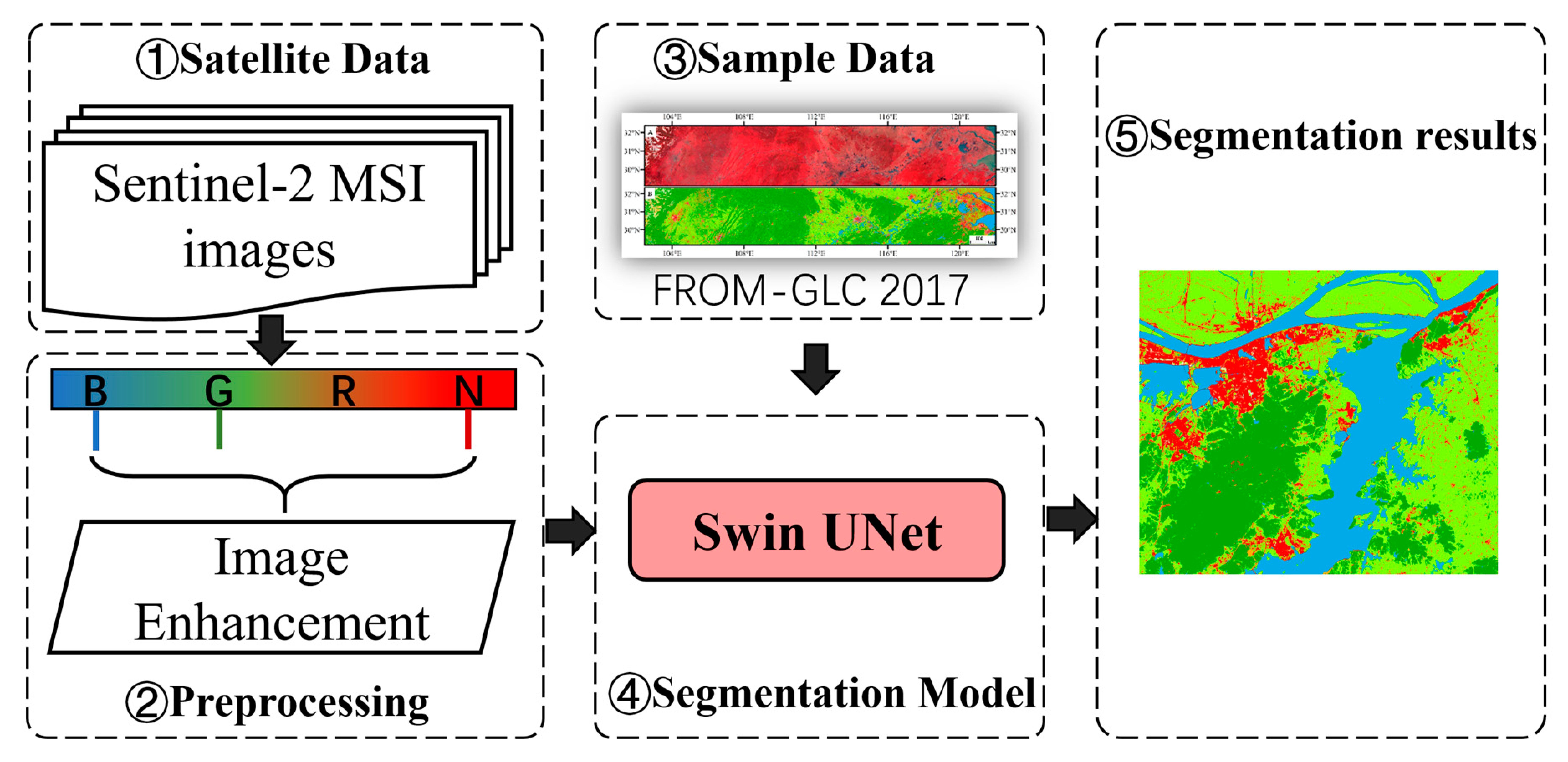
The SwinUnet model is improved and applied in a 10-categories segmentation from Sentinel-2 images, which is compared with traditional classification methods and CNN-based segmentation methods.

(2)

The FROM-GLC10 dataset is optimized and used as sample data. The approach and the transformer performance are analyzed.

(3)

The segmentation results of different spectral combinations from Sentinel-2 MSI (Multi-Spectral Imager) images are systematically compared and the optimal spectral combination scheme is obtained.

2. Data and Methods

2.1. Study Areas and Data

The satellite data used in the experiment are Sentinel-2 MSI optical images de-clouded and synthesized on Google Earth Engine (GEE). Label data is based on the FROM-GLC2017 dataset by the team at Tsinghua University [39], which can be obtained from http://data.ess.tsinghua.edu.cn/ (accessed on 3 July 2022). They defined the concept of stable classification and produced a global LULC product with 10 m resolution in 2017 with the Landsat-8 sample data in 2015. The categories included the cropland, forest, grassland, shrubland, wetland, water, tundra, impervious, bare land, and snow. The classification method used was the RF algorithm with the input features including the spectral values of Sentinel-2 data, indices of vegetation, water, building, and snow in classifying Landsa-8 data, slope and aspect data extracted from the SRTM elevation data, and the geographical coordinates. Eventually, the overall accuracy on the 2015 validation sample was 72.76%. We selected a zone from 29°36′ to 32°18′ latitude and 103°5′ to 121°45′ in the midland of China, with a ground resolution of 10 m. The pseudo-color composite satellite image is shown in Figure 1A, and the produced label data is shown in Figure 1B. The sample data in this paper are beneficial for the training and validation of multi-class segmentation of medium-resolution remote sensing images, because the latitude of the study area is suitable and the distance between land and sea is long, which makes the features obvious and covers all categories. In addition, we manually extracted a large number of validation points to prove the reliable accuracy of the area label data. Moreover, such a large amount of data enable the transformer model to be trained effectively. Because the label data are the corresponding cartographic products of 2017, we selected the satellite images of the same time and produced a total of 29,218 512 × 512-pixel tiles after uniform cropping and filtering. To train and evaluate the network model, the data is divided into the training set, validation set, and test set in the ratio of 80%, 10%, and 10%, respectively.

The channels of the input images are the focus of the experimental comparison in this paper. All the spectral channels of Sentinel-2 with 10 m resolution used in the experiment are listed in

Table 1. Sentinel-2 data used for study.

Band Number	Band Name	Central Wavelength (μm)	Resolution (m)
B2	Blue (B)	0.49	10
B3	Green (G)	0.56	10
B4	Red (R)	0.66	10
B8	Near Infrared (N)	0.84	10

, including Blue (B), Green (G), Red (R), and Near Infrared (N). Finally, we compare three spectral combination methods, namely R + G + B, N + G + B, and N + R + G + B.

2.2. Technical Route and Swin UNet

The main process steps and methods used in this paper are shown in Figure 2A. First, the 2017 cloud-free Sentinel-2 MSI images were screened on the GEE platform with cropping into a uniform size, and defective pixels were removed. The spectral selection module is responsible for dividing the input multi-band images into different combinations of bands as input to the network. To get better robustness of the model, we added image enhancement processing, including small-angle rotation and HSV (Hue, Saturation, and Value) transform. Finally, after a series of processing, the images were fed into the trained Swin UNet model for forwarding propagation, and the results of multi-category segmentation were obtained.

The well-established CNN-based segmentation models are used as comparisons, including two segmentation models and four backbone networks. UNet is proposed on the basis of FCN, using a combination of multilayer downsampling and upsampling with skip connection to reduce semantic information loss, which enables UNet to perform well on lightweight data. The DeepLabV3+ model is also based on the encoder-decoder architecture, which uses Atrous Separable Convolution to optimize the information between space and channels to reduce computational complexity and the pyramid module to obtain multi-scale convolutional features. In addition, CNN backbone networks with different depths and structures can be used on these segmentation models to achieve different segmentation performance, including VGG, ResNet50, MobileNet, and Xception used in the paper. VGG uses multiple convolutional layers with smaller convolutional kernels (3 × 3) instead of one convolutional layer with a larger convolutional kernel; the layers are separated from each other using max-pooling with a 2 × 2 pooling kernel, and the activation units of all hidden layers use the ReLU function. ResNet introduces the residual structure, so that the network layer can realize identity mapping and solve the problem of the gradient disappearing. ResNet50 goes through 4 blocks, with 3, 4, 6, and 3 bottlenecks in each block, respectively. MobileNet is a lightweight network proposed by Google in 2016, using depth-separable modules instead of convolutional operations to achieve faster computing speed, and the whole network is actually a stack of depth-separable modules. Similar to MobileNet, the Xception network also uses depthwise separable convolution, which is an extreme Inception network, by separating the correlation between channels from spatial correlation.

The architecture of the Swin UNet model is shown in Figure 2B. The whole network structure is similar to the original UNet, consisting of an encoder, bottleneck, decoder, and skip connection. The encoder part uses the backbone network of the Swin Transformer (a four-layer hierarchy), with each layer consisting of patch merging and a Swin Transformer block. Its design concept comes from the idea of a CNN-based network, patch merging, which is equivalent to a pooling operation and responsible for downsampling, and a Swin Transformer block, which is responsible for extracting features as a CNN. Since the minimum structured unit of Swin Transformer is a 4 × 4 image element, the input image becomes 1/4 of the original length and width and 16 times the original channel after the patch partition process. The structure of the first layer in the encoder is the same as that of VIT using a linear embedding connection, which does not change the length and width but makes the channels twice, and during the subsequent three layers of downsampling the length and width are reduced by half each time and the channels become twice as large. The decoder structure is symmetrically opposite to an encoder using patch expanding layers for upsampling. The first three upsampling layers are used to reshape the low-resolution feature mapping into twice the high-resolution feature mapping and correspondingly reduce the feature dimension to half of the original dimension. To keep the output image the same size as the input image, the last patch expanding layer is upsampled 4 times in length and width and the channel is not changed. Unlike the encoder’s Swin Transformer block, the decoder’s Swin Transformer block accepts two inputs, which are the features of upsampling and skip connection. The extracted contextual features are able to be fused with the multi-scale features of the encoder through a skip connection to complement the loss of spatial information due to downsampling.

Different from the conventional Multi-Head Self-Attention (MSA) module used in VIT, the Swin Transformer block can be thought as a series of two modules. As shown in Figure 2C, a Swin Transformer block consists of a regular Window-Based MSA (W-MSA) module and a Shifted Window-Based MSA(SW-MSA) module, followed by a 2-layer Multilayer Perceptron (MLP) with Gaussian Error Linear Units (GELU) nonlinearity. A LayerNorm (LN) layer is applied before each MSA module and each MLP, and a residual connection is applied after each module [40]. The detailed calculation rules are as follows.

$${\widehat{z}}^l=\mathit{W-MSA}\left(LN\left(z^{l-1}\right)\right)+z^{l-1}$$

(1)

$$z^l=MLP\left(LN({\widehat{z}}^l)\right)+{\widehat{z}}^l$$

(2)

$${\widehat{z}}^{l+1}=\mathit{SW-MSA}\left(LN(z^l)\right)+z^l$$

(3)

$$z^{l+1}=\mathit{W-MSA}\left(LN({\widehat{z}}^{l+1})\right)+{\widehat{z}}^{l+1}$$

(4)

where ${\widehat{z}}^l$ is the output features of the (S)W-MSA module and $z^l$ is the output features of the MLP module, where $l$ represents the number of blocks.

2.3. Network Enhancement Methods

The image enhancement step in network training can effectively improve the performance of the model in all aspects and also make more efficient use of the training data [41]. In this paper, two main enhancements are made to the picture of the input model. On the one hand, the length and width of the original image are randomly scaled up or down by a factor of 0.7 to 1.3 and randomly pasted onto a 512 × 512 grayscale image (grayscale image here implies a pixel value of 128). Rotation and flip were not used for medium-resolution remote sensing images, and features are generally not affected by these. On the other hand, the input image needs to undergo an HSV transform, which transforms the image into the HSV domain and back again. In the HSV domain, the hue channel does a random change of ±0.1 amplitude, while the saturation and value channels do a random change of ±0.5 amplitude. The reason is that medium-resolution remote sensing images often cover a wide area, which leads to the need for multiple images to cover the study area, and there are color differences between images of different frames due to different imaging times. The enhancement of the HSV conversion process improves the robustness of the model.

The loss function describes the size of the difference between the predicted and true values of the model, which is the key to determining the quality of network learning [42]. However, the categories in the medium-resolution remote sensing image segmentation task are diverse and varied, resulting in a strong imbalance between positive and negative samples. The dice loss function proposed in the article VNet [43] is a good solution to this problem. The calculation of the dice coefficient is equivalent to the F1-score, which means that it can be optimized well for the F1-score. However, the dice loss tends to be unstable in training, especially in the case of small targets, and extreme cases can lead to gradient saturation phenomena. Therefore, the combined dice loss with CE (Cross-Entropy) loss is improved to solve this problem well, and the loss function of this paper is calculated as follows.

$$Los{s}_{total}=los{s}_{CE}+(1-los{s}_{dice})$$

(5)

2.4. Evaluation Metrics

In order to evaluate the performance of our model effectively, Mean Intersection Over Union (MIOU), F1-score, and accuracy parameters were used for validation. The equations for each parameter and intermediate variables are calculated as follows.

$$MIOU=\frac{1}{N+1}{\displaystyle \sum }_{i=0}^{N}IOU$$

(6)

$$IOU=\frac{TP}{TP+FN+FP}$$

(7)

$$\mathrm{F1-score}=\frac{2\times Precsion\times Recall}{Precsion+Recall}$$

(8)

$$Precsion=\frac{TP}{TP+FP}$$

(9)

$$Recall=\frac{TP}{TP+FN}$$

(10)

$$\mathrm{Accuracy}=\frac{TP+TN}{TP+TN+FP+FN}$$

(11)

In all formulas, TP represents true positive, where the model correctly predicts the positive class. FP represents false positive, where the model incorrectly predicts the positive class. TN represents true negative, where the model predicts the negative class correctly. FN represents a false negative, where the model incorrectly predicts the negative class. N in Equation (7) represents the number of categories, which is set to 10 in this paper. $Precsion$ and $Recall$ in Equation (8) are calculated as shown in Equations (9) and (10).

2.5. Experimental Environment

Computer hardware: the CPU is an AMD 3800X, and the GPU is an NVIDIA Geforce RTX 2070 super 8G. Computer Software: Python version is 3.7.2, the PyTorch version is 1.4.0, and the CUDA version is 11.4. Parameter Configuration: the batch size is set to 4, the learning rate is 0.00001, and the maximum number of iterations is set to 100 rounds.

3. Results and Validations

3.1. Results and Comparison with CNN-Based Networks

After uniform training, different classical CNN-based networks were selected to evaluate the results of the test set together with our model. As the 10-categories segmentation evaluation metrics of each model on Sentinel-2 images shows in

Table 2. Performance comparison of different methods in Sentinel-2 images 10-categories segmentation *.

Item	Backbone	MIOU (%)	Accuracy (%)	F1-Score (%)
UNet	VGG	70.6	85.05	69.84
	ResNet50	67.73	82.73	66.93
DeeplabV3+	MobileNet	70.47	86.58	72.91
	Xception	69.2	82.44	71.63
Swin-UNet	Swin Transformer	72.06	89.77	76.46

* MIOU = Mean Intersection Over Union.

, the Swin UNet-based method in this paper outperforms all CNN-based methods in each evaluation metric. In the medium-resolution remote sensing image segmentation task, the model based on UNet and DeeplabV3+ framework performs similarly, but the different backbone networks have a greater impact on the accuracy of the results. In the DeeplabV3+ model, MobileNet has a 4.14% improvement in accuracy and a slight improvement in MIOU and F1-score when compared to Xception. The same phenomenon occurs in the UNet model, where the VGG performs better than ResNet50, with a 2.32% improvement in accuracy and slightly larger improvements in the MIOU and F1-score, reaching 2.87% and 2.91%. The results based on the Swin Transformer backbone network exceed the performance of VGG and outperform all models of DeeplabV3+. The results also outperform VGG by 4.72% based on the Swin Transformer backbone network and by more than 3% over the second-highest accuracy based on all other models and also have the highest overall MIOU and F1-score metrics.

The results in Table 2 show that the lighter backbone networks perform better in medium-resolution remote sensing images, just as VGG outperforms RESNet50 and MobileNet outperforms Xception. Although a huge number of training image datasets were chosen, the lightweight backbone networks are found to fit faster with stable accuracy improvement, while the deeper structured ResNet50 and Xception backbone networks fit slowly with fluctuating accuracy, which is one of the reasons for their poor results. In addition, for medium-resolution remote sensing images, the spatial information is insufficient when compared to high-resolution remote sensing images, which means that a larger and deeper network structure is not an effective way to improve segmentation accuracy [44], while transformer provides an alternative path using the global self-attention mechanism, and experimental results also show that our method compensates well for the shortcomings of medium-resolution remote sensing images and achieves the highest performance.

It can also be seen in the comparison of the results in Figure 3 (where the black arrow points) that our results have better segmentation performance when compared to other methods. Comparing with the satellite images, it can be seen that the refinement of road segmentation and the recognition of small water ponds are well done in our results, while roads were not well extracted in the ResNet50 results; small ponds and small plowed areas were also misclassified as impervious surfaces in Xception. In addition, our model has a good ability to discriminate features close to the edges, such as in the segmentation of the river where the missing edge river phenomenon occurs in the CNN-based model. It is important to mention that since our Label data is classified via the random forest method based on image pixels, and there are some noise points and misclassification in it our model achieves better robustness and discriminatory ability after training with a large number of samples. This can also be seen from the final segmentation result of the mountain valley, and our model successfully identifies small settlements, which are not identified by label data.

In order to study the effect of each category on the overall accuracy, we calculated statistics for three metrics of 10 categories, the results of which are shown in

Table 3. 10-categories accuracy statistics *.

Class	IOU (%)	Recall (%)	Precision (%)
Crop	82.01	93.84	86.68
Forest	82.06	93.07	87.4
Grassland	34.22	38.41	62.19
Shrubland	64.23	70.3	77.11
Wetland	36.36	43.15	60.12
Water	86.22	91.46	93.78
Tundra	33.89	41.66	70.48
Impervious land	59.62	72.24	77.34
Bare land	38.5	42.1	73.17
Snow/Ice	29.9	33.64	68.33

* IOU = Intersection Over Union.

. The IOUs of crop, forest, and water all performed well, while impervious land was slightly lower, which could be due to the wide distribution and irregular shape of impervious surfaces. However, grassland, shrubland, wetland, tundra, bare land, and snow/ice all have lower IOUs because the distribution of these categories is very small throughout the study area, which also means that the training sample is insufficient, but a small number of segmentation inaccuracies have little effect on the overall accuracy. The IOU metrics in Table 3 are lower than the recall and precision metrics, partly because up to 10 categories of segmentation tasks can lead to the occurrence of interclass errors, partly because the distribution of features in some categories is very irregular and the label data itself is inaccurate.

3.2. Results of Large-Scale Mapping

Large-scale land use mapping is an important application of semantic segmentation models in the field of remote sensing. In this paper, we intend to demonstrate the great potential of our method in large-scale mapping and the results of our model and other CNN-based models. Figure 4 shows a relatively comprehensive range of surface objects in the city of Jiujiang. The distribution of categories in our results is roughly the same as in label data. It is worth noting that our model did not show the phenomenon of mountain shadows misclassified into water bodies when compared to the CNN-based model, which is marked with the red box in the figure. Using the transformer’s self-attentive mechanism, our model embraces the global features, which outperforms the limited perceptual field of the CNN-based model. In addition, the fine rivers and roads are well segmented, which shows that our model has good spatial detail extraction ability. Our results are clean and focused for each category of blocks with clear boundaries of water bodies and good details of impervious surfaces. However, for the recognition of the category of urban green space, our model is inferior to Mobilenet, which requires subsequent targeted training.

3.3. Different Image Band Combinations

Sentinel-2 has four spectral bands with 10 m resolution, while the common network inputs are RGB images. From the multispectral processing of remote sensing images, it is necessary to study different spectral combinations. Based on previous studies [45], the three most commonly used spectral combination methods are selected as the input to the network in this paper. After uniform training, the performance of different methods on the test set is shown in

Table 4. 10-categories segmentation results of band combinations in Sentinel-2 images *.

Band Combinations	MIOU (%)	Accuracy (%)	F1-Score (%)
RGB	71.30	86.31	72.09
NGB	72.06	89.77	76.46
NRGB	69.92	82.86	70.68

* MIOU = Mean Intersection Over Union, B = Blue, G = Green, R = Red, and N = Near Infrared.

.

During the training process, both RGB and NGB enter convergence faster and the accuracy continues to improve. In contrast, NRGB starts the training with a large fluctuation in loss and soon fails to continue the improvement. It can be seen that having a lot of spectral features does not necessarily improve the performance of the model, and the replacement of the red band with NIR can effectively improve a part of the model’s performance in medium-resolution remote sensing segmentation. In addition, multi-channel input images are not accessible to many classical three-channel image enhancements (e.g., HSV conversion), which is partly responsible for this.

4. Discussion

4.1. Impact Factors of Accuracy

Our training samples are from the FROM-GLC10 dataset, which has 72.76% accuracy based on the validation samples in Gong et al. (2019). The accuracy in this study area is slightly higher as illustrated by our own validation sample. However, there are still some problems, such as severe noise due to the image pixel-based classification method and some misclassified parts (mountain shadows, water edges, etc.) due to the outdated classifier. In addition, FROM-GLC10 was obtained based on sample training at 30 m resolution, which leads to some strange lumpy category distributions in its results. These issues can cause problems for network training, where these errors are simply ignored and treated as true values for participation in training. Therefore, we used 4898 visually interpreted sample points to verify the segmentation accuracy of the Swin UNet model, and some categories (shrubland and tundra) were not included because there were no available data. As shown in

Table 5. Accuracy validation of the Swin UNet model based on visually interpreted samples *.

Class	Crop	Forest	Grassland	Water	Impervious Land	Bareland	Snow/Ice	Wetland	UA (%)
Crop	656	18	0	0	0	0	0	0	97.33
Forest	34	486	0	0	0	0	0	0	93.46
Grassland	0	132	199	2	0	0	1	0	59.58
Water	32	1	0	322	11	0	0	19	83.64
Impervious land	25	24	0	0	900	0	0	20	92.88
Bare land	14	20	47	0	67	715	1	37	79.36
Snow/ice	0	1	2	9	0	0	606	8	96.81
Wetland	83	16	16	22	0	22	60	270	55.21
PA (%)	77.73	69.63	75.38	90.70	92.02	97.01	90.72	76.27
OA (%): 84.81					Kappa coefficient: 0.82

* UA = User’s Accuracy, PA = User’s Accuracy, OA = Overall Accuracy.

, an overall accuracy of 84.81% with a kappa coefficient of 0.82 was achieved via the validation of the sample points visually interpreted, which proves the accuracy of our results. In addition, it also shows that stable classification results can be obtained with limited accuracy of training samples, which is consistent with the experimental results of Gong, et al. [39]. The results are quite satisfactory, and the errors in label data are corrected for our results with successful segmentation of the area of small settlements that appears in label data (Figure 3). This is probably due to the possibility that we expanded the training data and added image enhancement to counteract this effect.

On the other hand, the classification system used in this paper follows the 10 categories (cropland, forest, grassland, shrubland, wetland, water, tundra, impervious, bare land and snow) in label data. However, in the analysis of the results (Figure 5), we found that some of the categories (grassland, wetland, tundra, and snow) are very small and unbalanced, and adding dice loss cannot completely solve the impact of the low accuracy of these categories on the overall accuracy. Therefore, we tried to group these sparsely distributed categories into the backgrounds and finally obtained the highest precision of 91.02% with 6 categories (cropland, forest, shrubland, water, impervious, and bareland). The accuracy is not much improved because of the limitation of label data. However, by observing their loss curves, it can be seen that the model of 6 categories has a lower validation loss when compared to that of 10 categories, which indicates a more stable model. The network learns faster by completing the iterations in 80 rounds.

4.2. Migrability of the Segmentation Model

Most validation data for remote sensing image segmentation are in the same study area as the training data, which cannot prove the segmentation model’s robustness. Although many segmentation models have high accuracy on their own validation data, they do not work well when applying it to other regions, which is caused by an insufficient training sample size or insufficient fitting ability of the model. With such a large and robust training sample coupled with excellent models, we believed that this would advance land use mapping efforts on a global scale. To test this idea, the land use mapping work for two regions, Washington and Beijing, was carried out, which is shown in Figure 6. Overall, the categories of crop, forest, water, and impervious surfaces were well extracted in both results by comparing with satellite images. However, the impervious surface extraction for the Washington area was not as effective as for the Beijing area, where some areas of the crop were confused with impervious surfaces. This may be due to the fact that our training samples were all within China, and the urban structure of the US is very different from that of China.

4.3. Limitations and Outlooks

In this paper, we investigated the utility of a semantic segmentation model based on the Swin-UNet model for medium-resolution remote sensing images. After the large volume of training data were produced, the transformer model was well fitted. For the complex 10-categories segmentation task, our model achieved higher performance when compared to the CNN-based approach. Another point is that the spectral selection module was well applied and had some improvement in the transformer model performance. Although the Transform method provides a new way to classify medium-resolution remote sensing images, there is still a need to improve its extraction capability for local features. In the future, we will further investigate other transformer-based network models for comparison and try larger segmentation tasks, such as global land use mapping.

5. Conclusions

Medium-resolution remote sensing satellite images are important for environmental monitoring and climate change research. The accuracy of large-scale land use mapping depends greatly on the performance of the segmentation model. In this paper, the Swin-UNet model was improved and successfully applied to the multi-category segmentation task for medium-resolution remote sensing images and excellent performances were achieved. The experimental results show that (1) the Swin-UNet model performs well in the 10-categories image segmentation task in the medium-resolution Sentinel-2 MSI optical images with an MIOU of 72.06%, an accuracy of 89.77%, and an F1-score of 76.46%. (2) Comparing with other CNN-based models, including DeepLabV3+ and U-Net, and different backbone networks, including VGG, ResNet50, MobileNet, and Xception, the reliable results of our model are obtained in the medium-resolution remote sensing image segmentation task. (3) Different spectral combinations as the input of the network have certain effects on the performance of the network, and the replacement of the red-light band with the near-infrared band has an enhancement effect on the transformer-based model. In addition, the Swin-UNet model also shows good performance in model transfer.

References

1. Hansen, M.C.; Loveland, T.R. A review of large area monitoring of land cover change using Landsat data. Remote Sens. Environ. 2012, 122, 66–74. [Google Scholar] [CrossRef]
2. Foley, J.A.; DeFries, R.; Asner, G.P.; Barford, C.; Bonan, G.; Carpenter, S.R.; Chapin, F.S.; Coe, M.T.; Daily, G.C.; Gibbs, H.K. Global consequences of land use. Science 2005, 309, 570–574. [Google Scholar] [CrossRef] [PubMed] [Green Version]
3. Vorosmarty, C.J.; McIntyre, P.B.; Gessner, M.O.; Dudgeon, D.; Prusevich, A.; Green, P.; Glidden, S.; Bunn, S.E.; Sullivan, C.A.; Liermann, C.R.; et al. Global threats to human water security and river biodiversity. Nature 2010, 467, 555–561. [Google Scholar] [CrossRef] [PubMed]
4. Findell, K.L.; Berg, A.; Gentine, P.; Krasting, J.P.; Lintner, B.R.; Malyshev, S.; Santanello, J.A., Jr.; Shevliakova, E. The impact of anthropogenic land use and land cover change on regional climate extremes. Nat. Commun. 2017, 8, 989–990. [Google Scholar] [CrossRef]
5. Haddeland, I.; Heinke, J.; Biemans, H.; Eisner, S.; Florke, M.; Hanasaki, N.; Konzmann, M.; Ludwig, F.; Masaki, Y.; Schewe, J.; et al. Global water resources affected by human interventions and climate change. Proc. Natl. Acad. Sci. USA 2014, 111, 3251–3256. [Google Scholar] [CrossRef] [Green Version]
6. Zhu, Z.; Wulder, M.A.; Roy, D.P.; Woodcock, C.E.; Hansen, M.C.; Radeloff, V.C.; Healey, S.P.; Schaaf, C.; Hostert, P.; Strobl, P.; et al. Benefits of the free and open Landsat data policy. Remote Sens. Environ. 2019, 224, 382–385. [Google Scholar] [CrossRef]
7. Kauth, R.J.; Thomas, G.S. The tasselled cap—A graphic description of the spectral-temporal development of agricultural crops as seen by Landsat. Mach. Process. Remote. Sens. Data 1976, 159, 41–51. [Google Scholar]
8. Pekel, J.F.; Cottam, A.; Gorelick, N.; Belward, A.S. High-resolution mapping of global surface water and its long-term changes. Nature 2016, 540, 418–422. [Google Scholar] [CrossRef]
9. Huang, X.; Li, J.; Yang, J.; Zhang, Z.; Li, D.; Liu, X. 30 m global impervious surface area dynamics and urban expansion pattern observed by Landsat satellites: From 1972 to 2019. Sci. China Earth Sci. 2021, 64, 1922–1933. [Google Scholar] [CrossRef]
10. Hansen, M.C.; Potapov, P.V.; Moore, H.; Turubanova, S.A.; Tyukavina, T. High-Resolution Global Maps of 21st-Century Forest Cover Change. Science 2013, 342, 850–853. [Google Scholar] [CrossRef] [Green Version]
11. Yuan, W.; Xu, W. MSST-Net: A Multi-Scale Adaptive Network for Building Extraction from Remote Sensing Images Based on Swin Transformer. Remote Sens. 2021, 13, 4743. [Google Scholar] [CrossRef]
12. Vapnik, V.N.; Chervonenkis, A.Y. On a perceptron class. Avtomat. Telemekh. 1964, 1964, 112–120. [Google Scholar]
13. Breiman, L. Random Forests. Mach. Learn. 2001, 45, 5–32. [Google Scholar] [CrossRef] [Green Version]
14. Zhang, X.; Liu, L.; Chen, X.; Gao, Y.; Xie, S.; Mi, J. GLC_FCS30: Global land-cover product with fine classification system at 30 m using time-series Landsat imagery. Earth Syst. Sci. Data 2021, 13, 2753–2776. [Google Scholar] [CrossRef]
15. Yang, J.; Huang, X. The 30 m annual land cover dataset and its dynamics in China from 1990 to 2019. Earth Syst. Sci. Data 2021, 13, 3907–3925. [Google Scholar] [CrossRef]
16. Gong, P.; Wang, J.; Yu, L.; Zhao, Y.; Chen, J. Finer resolution observation and monitoring of global land cover: First mapping results with Landsat TM and ETM+ data. Int. J. Remote Sens. 2013, 34, 2607–2654. [Google Scholar] [CrossRef] [Green Version]
17. Moser, G.; Serpico, S.B.; Benediktsson, J.A. Land-Cover Mapping by Markov Modeling of Spatial–Contextual Information in Very-High-Resolution Remote Sensing Images. Proc. IEEE 2013, 101, 631–651. [Google Scholar] [CrossRef]
18. Zhu, X.X.; Tuia, D.; Mou, L.; Xia, G.S.; Zhang, L.; Xu, F.; Fraundorfer, F. Deep Learning in Remote Sensing: A Comprehensive Review and List of Resources. IEEE Geosci. Remote Sens. Mag. 2018, 5, 8–36. [Google Scholar] [CrossRef] [Green Version]
19. Lecun, Y.; Bottou, L. Gradient-based learning applied to document recognition. Proc. IEEE 1998, 86, 2278–2324. [Google Scholar] [CrossRef] [Green Version]
20. Zhang, L.; Zhang, L.; Bo, D. Deep Learning for Remote Sensing Data: A Technical Tutorial on the State of the Art. IEEE Geosci. Remote Sens. Mag. 2016, 4, 22–40. [Google Scholar] [CrossRef]
21. Huang, G.; Liu, Z.; Laurens, V.; Weinberger, K.Q. Densely Connected Convolutional Networks. In Proceedings of the IEEE Conference on Computer Vision and Pattern Recognition, Honolulu, HI, USA, 21–26 July 2017; pp. 4700–4708. [Google Scholar]
22. Xie, S.; Girshick, R.; Dollár, P.; Tu, Z.; He, K. Aggregated Residual Transformations for Deep Neural Networks. In Proceedings of the IEEE Conference on Computer Vision and Pattern Recognition, Honolulu, HI, USA, 21–26 July 2017; pp. 1496–1500. [Google Scholar]
23. Krizhevsky, A.; Sutskever, I.; Hinton, G.E. Imagenet classification with deep convolutional neural networks. Adv. Neural Inf. Process. Syst. 2012, 25, 84–90. [Google Scholar] [CrossRef]
24. Simonyan, K.; Zisserman, A. Very Deep Convolutional Networks for Large-Scale Image Recognition. Comput. Sci. 2014, 30, 330–335. [Google Scholar]
25. He, K.; Zhang, X.; Ren, S.; Sun, J. Deep Residual Learning for Image Recognition. In Proceedings of the IEEE Conference on Computer Vision and Pattern Recognition, Las Vegas, NV, USA, 26 June–1 July 2016; pp. 770–778. [Google Scholar]
26. Chollet, F. Xception: Deep Learning with Depthwise Separable Convolutions. In Proceedings of the IEEE Conference on Computer Vision and Pattern Recognition, Honolulu, HI, USA, 21–26 July 2017; pp. 1251–1258. [Google Scholar]
27. Long, J.; Shelhamer, E.; Darrell, T. Fully Convolutional Networks for Semantic Segmentation. IEEE Trans. Pattern Anal. Mach. Intell. 2015, 39, 640–651. [Google Scholar]
28. Ronneberger, O.; Fischer, P.; Brox, T. U-Net: Convolutional Networks for Biomedical Image Segmentation. In Proceedings of the International Conference on Medical Image Computing and Computer-Assisted Intervention, Munich, Germany, 5–9 October 2015; pp. 234–241. [Google Scholar]
29. Badrinarayanan, V.; Kendall, A.; Cipolla, R. SegNet: A Deep Convolutional Encoder-Decoder Architecture for Image Segmentation. IEEE Trans. Pattern Anal. Mach. Intell. 2017, 39, 2481–2495. [Google Scholar] [CrossRef]
30. Zhao, H.; Shi, J.; Qi, X.; Wang, X.; Jia, J. Pyramid Scene Parsing Network. In Proceedings of the IEEE Conference on Computer Vision and Pattern Recognition, Honolulu, HI, USA, 21–26 July 2017; pp. 2881–2890. [Google Scholar]
31. Wu, Z.; Chen, X.; Gao, Y.; Li, Y. Rapid Target Detection in High Resolution Remote Sensing Images Using YOLO Model. ISPRS-Int. Arch. Photogramm. Remote Sens. Spat. Inf. Sci. 2018, 42, 1915–1920. [Google Scholar] [CrossRef] [Green Version]
32. Cao, K.; Zhang, X. An improved res-unet model for tree species classification using airborne high-resolution images. Remote Sens. 2020, 12, 1128. [Google Scholar] [CrossRef] [Green Version]
33. Gao, L.; Liu, H.; Yang, M.; Chen, L.; Xiao, Z. STransFuse: Fusing Swin Transformer and Convolutional Neural Network for Remote Sensing Image Semantic Segmentation. IEEE J. Sel. Top. Appl. Earth Obs. Remote Sens. 2021, 14, 10990–11003. [Google Scholar] [CrossRef]
34. Guo, Y.; Liao, J.; Shen, G. A deep learning model with capsules embedded for high-resolution image classification. IEEE J.-Stars 2020, 14, 214–223. [Google Scholar] [CrossRef]
35. Vaswani, A.; Shazeer, N.; Parmar, N.; Uszkoreit, J.; Jones, L.; Gomez, A.N.; Kaiser, Ł.; Polosukhin, I. Attention is all you need. Adv. Neural Inf. Process. Syst. 2017, 30, 1–11. [Google Scholar]
36. Dosovitskiy, A.; Beyer, L.; Kolesnikov, A.; Weissenborn, D.; Zhai, X.; Unterthiner, T.; Dehghani, M.; Minderer, M.; Heigold, G.; Gelly, S. An image is worth 16x16 words: Transformers for image recognition at scale. arXiv 2020, arXiv:2010.11929. [Google Scholar]
37. Zheng, S.; Lu, J.; Zhao, H.; Zhu, X.; Zhang, L. Rethinking Semantic Segmentation from a Sequence-to-Sequence Perspective with Transformers. In Proceedings of the IEEE Conference on Computer Vision and Pattern Recognition, Virtual, 19–25 June 2021; pp. 6881–6890. [Google Scholar]
38. Cao, H.; Wang, Y.; Chen, J.; Jiang, D.; Zhang, X.; Tian, Q.; Wang, M. Swin-unet: Unet-like pure transformer for medical image segmentation. arXiv 2020, arXiv:2105.05537. [Google Scholar]
39. Gong, P.; Liu, H.; Zhang, M.; Li, C.; Wang, J.; Huang, H.; Clinton, N.; Ji, L.; Li, W.; Bai, Y.; et al. Stable classification with limited sample: Transferring a 30-m resolution sample set collected in 2015 to mapping 10-m resolution global land cover in 2017. Sci. Bull. 2019, 64, 370–373. [Google Scholar] [CrossRef] [Green Version]
40. Liu, Z.; Lin, Y.; Cao, Y.; Hu, H.; Wei, Y.; Zhang, Z.; Lin, S.; Guo, B. Swin transformer: Hierarchical vision transformer using shifted windows. In Proceedings of the IEEE/CVF International Conference on Computer Vision, Montreal, QC, Canada, 11–17 October 2021; pp. 10012–10022. [Google Scholar]
41. Filip, R.; Giorgos, T.; Ondrej, C. Fine-tuning CNN Image Retrieval with No Human Annotation. IEEE Trans. Pattern Anal. Mach. Intell. 2017, 41, 1655–1668. [Google Scholar]
42. Chen, L.; Qu, H.; Zhao, J.; Chen, B.; Principe, J.C. Efficient and robust deep learning with Correntropy-induced loss function. Neural Comput. Appl. 2016, 27, 1019–1031. [Google Scholar] [CrossRef]
43. Milletari, F.; Navab, N.; Ahmadi, S.A. V-Net: Fully Convolutional Neural Networks for Volumetric Medical Image Segmentation. In Proceedings of the 2016 Fourth International Conference on 3D Vision (3DV), Stanford, CA, USA, 25–28 October 2016; pp. 565–571. [Google Scholar]
44. Wang, X.; Ming, Y.U.; Ren, H.E. Remote sensing image semantic segmentation combining UNET and FPN. Chin. J. Liq. Cryst. Disp. 2021, 36, 475–483. [Google Scholar] [CrossRef]
45. Arbia, G.; Haining, G. Spatial error propagation when computing linear combinations of spectral bands: The case of vegetation indices. Environ. Ecol. Stat. 2003, 10, 375–396. [Google Scholar] [CrossRef]
Figure 1. Study area and data with the false-color composite satellite image (A) and the classified image (B).
Remotesensing 14 03382 g001
Figure 2. Flow chart of the method with the experimental flow (A), the network structure of Swin UNet (B), and the computational principle of Swin Transformer block (C). MSI = Multispectral Imager, MLP = Multilayer Perceptron, LN = Layer Norm, W-MSA = Window-Based Multi-Head Self-Attention, SW-MSA = Shifted Window-Based Multi-Head Self-Attention.
Remotesensing 14 03382 g002
Figure 3. Comparison of the results of different classification methods with rural (A), mountainous (B), riverine (C), and urban (D).
Remotesensing 14 03382 g003
Figure 4. Results of different networks for large scale mapping in Jiujiang.
Remotesensing 14 03382 g004
Figure 5. Loss curve for 6 categories (A) (including cropland, forest, shrubland, water, and impervious and bare land) and 10 categories (B) (including cropland, forest, grassland, shrubland, wetland, water, tundra, impervious and bare land, and snow).
Remotesensing 14 03382 g005
Figure 6. Large-scale mapping of other regions in Washington D.C. (A) and Beijing (B).
Remotesensing 14 03382 g006