Article

Analysis of PM2.5 Variations Based on Observed, Satellite-Derived, and Population-Weighted Concentrations

1
School of Municipal and Geomatics Engineering, Hunan City University, Yiyang 413000, China
2
School of Geosciences and Info-Physics, Central South University, Changsha 410083, China
*
Author to whom correspondence should be addressed.
Remote Sens. 2022, 14(14), 3381; https://doi.org/10.3390/rs14143381
Submission received: 19 May 2022 / Revised: 24 June 2022 / Accepted: 11 July 2022 / Published: 14 July 2022

Abstract

:
Fine particulate matter (PM2.5), which can cause adverse human health effects, has been proven as the first air pollutant in China. In situ observations with ground-level monitoring and satellite-based concentrations have been used to analyze the variations in PM2.5. However, variation analyses based on these two kinds of measurement have mainly focused on the concentration itself and ignored the effects on the population. Therefore, this study not only investigated these two kinds of measurements, but also performed weighted population analyses to study the variations in PM2.5. Firstly, daily models of timely structure adaptive modeling (TSAM) were constructed to simulate satellite-derived PM2.5 levels from January 2013 to December 2016. Secondly, population-weighted concentrations were calculated based on TSAM-derived PM2.5 surfaces. Finally, observed, TSAM-derived, and population-weighted concentrations were used to analyze the variations in PM2.5. The results showed the different importance of various input parameters; AOD had the highest rank. Additionally, TSAM models demonstrated good performance, fitting R ranging from 0.86 to 0.91, and validating R from 0.82 to 0.89. According to the air quality standard in China, TSAM-derived PM2.5 showed that the increase in area lower than Level II was 29.03% and the increase in population was only 14.81%. This indicates that the air quality exhibited an overall improvement in spatial perspective, but some areas with high population density showed a relatively low improvement due to uneven distributions in China. The population-weighted PM2.5 concentration could better represent the health threats of air pollutants compared with in situ observations.

1. Introduction

Fine particulate matter (PM2.5) with micro particle sizes can cause serious health consequences, such as morbidity, mortality, and cardiovascular and respiratory diseases [1,2,3,4]. Except these hazards, it could also be the corrosion of materials [5]. With rapid economic development and urbanization in recent decades, China has been facing the growing problem of poor atmospheric environment [6,7]. Air pollution not only poses threats to public health but also affects daily production and life, such as atmospheric visibility reductions and the destruction of the urban landscape [7,8].
To improve air quality, national and local governments have promulgated a series of plans and policies since 2012. Among them are the 12th Five-Year Plan on Air Pollution Prevention and Control in Key Regions (abbreviation: Key Regions) and the most recent Chinese Ambient Air Quality Standard (CAAQS) released on 10 September 2013. At the same time, nationwide air quality monitoring networks have gradually been established since 2013. Increasing numbers of studies have been conducted to analyze the temporal–spatial variations in PM2.5 based on ground-level monitoring measurements [9,10,11].
However, site-based observations, which collect concentrations of air pollutants from fixed sites, merely reflect ambient PM2.5 concentrations at limited distances around the ground monitoring stations and hardly reflect spatial variations in air pollutants [12]. Additionally, researchers have focused on spatial interpolation methods to reveal regional variations in PM2.5, e.g., Kriging and inverse distance weight interpolation [13,14]. Spatial interpolation methods can derive surfaces of PM2.5 concentrations. However, the uncertainties in these methods could be high when varying topography, meteorology, and local emissions among the monitoring sites are not accounted for [14,15,16,17].
A previous study proved that remote sensing could provide more information about the Earth’s climate parameters (e.g., aerosols, temperature, pressure, etc.) [18]. Previous studies have proved that aerosol optical depth (AOD) and PM2.5 have similar particle sizes, which provide the theoretical basis of modeling between PM2.5 and satellite AOD [19,20]. At the same time, AOD with wide spatial coverage and acceptable accuracy which is satellite-retrieved can provide planar data from the macro scale and supplement ground observations. It has been increasingly utilized to simulate the regional distribution of PM2.5 [6,21,22]. Spatial–temporal statistical modeling is one of the most popular methods in PM2.5 concentration predictions and includes simple linear regression [23,24], multiple linear regression (e.g., land use regression (LUR) [14,17], geographically weighted regression (GWR) [21,25], linear mixed effect (LME) [26,27], timely structure adaptive modeling (TSAM) [22]), and artificial intelligence models (e.g., ANN) [16,28,29,30]. While the contributing strength of model predictors (i.e., variables) are allowed to change in these daily modeling process, all these models (no matter whether they are linear or non-linear) for individual days over a study period have a fixed structure. In fact, both the models’ predictors and their contributing strengths could vary with time. Then, TSAM takes temporal variations and magnitudes of predictors into consideration in the modeling process and provides a novel solution for continuously mapping the distributions of PM2.5 [22].
Existing research has mainly focused on the variations in in situ or satellite-derived concentrations of PM2.5 and then analyzed its spatial and temporal characteristics. Population density in China is not evenly distributed, and Hu demonstrated that 93.77% of the population live south-east of this “Hu Line”, which is a contrast line of population density proposed by Hu in 1935 [31]. Regions with high population density would therefore have higher population exposure risks with the same concentrations of pollutants. Additionally, when analyzing the effect of air pollution, we not only need to analyze concentration variations in air pollutants, but we also need to consider population exposure.
Therefore, the main aims of this study are: (1) to simulate the satellite-based distribution of PM2.5 from 2013 to 2016 with the TSAM modeling framework; (2) to analyze the spatial–temporal variations in observed and TSAM-derived PM2.5; and (3) to compare the difference between observed and population-weighted PM2.5 levels for Key Regions.

2. Materials and Methods
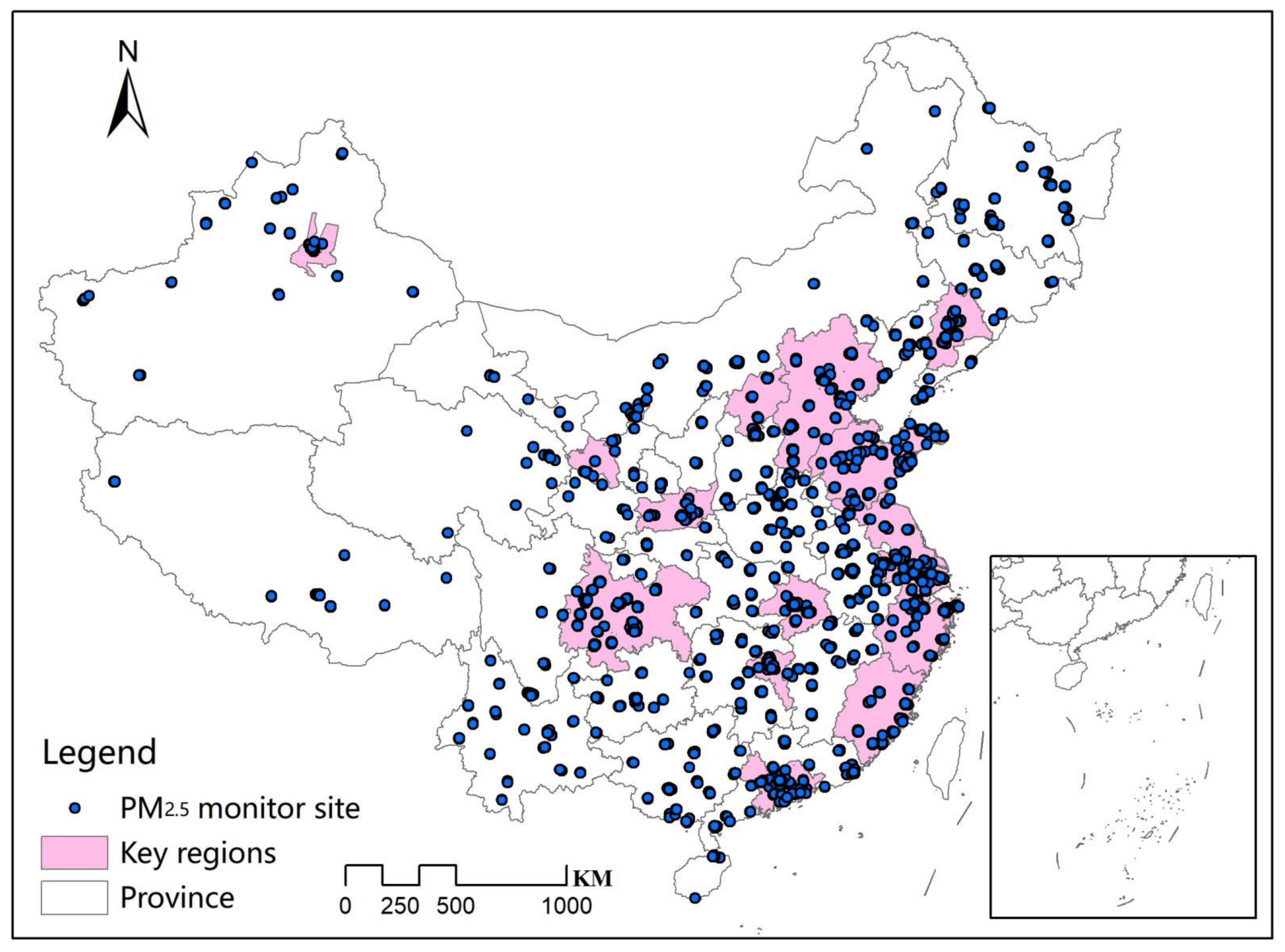
2.1. Study Area

This research selected mainland China as the study area (Figure 1), and especially the Key Regions, including the Beijing–Tianjin–Hebei Delta, the Yangtze River Delta, and the Pearl River Delta, as well as 10 city clusters (the cluster of Central Liaoning, Shandong Province, Wuhan region, Changsha–Zhuzhou–Xiangtan, Chengdu–Chongqing, Straits Fujian, central and northern areas of Shanxi, Shaanxi Guanzhong, and Gansu–Ningxia, and the city of Urumqi in Xinjiang).

2.2. Data Collection and Pre-Processing

2.2.1. In Situ Site-Based PM2.5 Measurements

Hourly ground PM2.5 concentrations were collected from the official database, which had 661 fixed sites in 2013 and 1436 by the end of 2016. These were measured with the tapered element oscillating microbalance method (TEOM). Invalid and error measurements caused by instrument calibration failure and power failure were reduced based on the Chinese National Ambient Air Quality Standards (CNAAQS, GB3095-2012). In this process, repeatedly reported records for several successive hours, significantly abnormal measurements (e.g., more than 1000 μg/m3 or less than 0 μg/m3), or fewer than 20 records of PM2.5 concentrations in a day were deleted. As a result, about 1% of records were discarded as abnormal during the study period. Screened hourly PM2.5 measurements were averaged into daily values for each monitoring station. To maintain a consistent spatial resolution of PM2.5 with the predictor of AOD, these daily PM2.5 values were recalculated based on the 10 km grid cells. Additionally, PM2.5 concentrations were calculated for grid cells with screened hourly observations which matched the satellite overpass times.

2.2.2. Satellite AOD

Moderate Resolution Imaging Spectroradiometer (MODIS) AOD products (National Aeronautics and Space Administration (NASA), Washington, DC, USA) are global MODIS Level 2 Aerosol Products Collection 6 (C6, NASA, Washington, DC, USA), which have been validated with AOD measurements from 33 Aerosol Robotic Network (AERONET, established by NASA, Washington, DC, USA, and PHOtométrie pour le Traitement Opérationnel de Normalisation Satellitaire, Lille, France) sites in China. The Level 2 C6 MODIS AOD of Terra (NASA, Washington, DC, USA, equatorial crossing time at 10:30 a.m.) and Aqua (equatorial crossing time at 13:30 p.m.) with a spatial resolution of 10 km were collected from 1 January 2013 to 31 December 2016. The combined Dark Target (DT) and Deep Blue (DB) AODs at 550 nm wavelength in C6 (MODIS parameter name: AOD_550_Dark_Target_Deep_Blue_Combined, NASA, Washington, DC, USA) with the highest quality assurance confidence flags (QA = 3) were screened as AOD values on specific days. To improve the spatial coverage, Terra AOD (MOD04) and Aqua AOD (MYD04) were extracted and combined, following an existing research method [22,32,33].

2.2.3. PM2.5 Emission Data

Due to the unavailability of the national emission inventory, land use, traffic networks, and demographic data were regarded as alternatives for indirectly characterizing the PM2.5 emissions. Population raster data with a resolution of 1 km in 2010 were collected and annually updated concerning the county-level population growth rate from 2013 to 2016. The variables of land use included the percentage of built-up area, forest area, grass area, and water area. The traffic variable was the total road length. Additionally, population density values were treated as proxy variables of demographic data.

2.2.4. PM2.5 Dispersion Conditions Data

It has been acknowledged that meteorology and topography are key factors that can directly influence the dispersion of PM2.5 [21,34]. About 900,000 daily meteorological records, including wind speed (WS, m/s), precipitation (PE, mm), relative humidity (RH, %), temperature (TEMP, K), and pressure (PS, hPa), were obtained from 824 sites of the meteorological monitoring network. Abnormal values were discarded in this process based on the quality control code and standard outlier elimination. These meteorological factors were interpolated with the inverse distance-weighted method into a 10 km raster. Moreover, as an indicator of topography, digital elevation model (DEM) data from the Shuttle Radar Topography Mission (SRTM) were collected with a spatial resolution of 90 m.

2.3. TSAM Modeling

2.3.1. Structure of the TSAM Model

TSAM, a model which has been proven to be effective in PM2.5 concentration estimations, was employed for satellite mapping in this study; details of TSAM were presented by Fang et al. [22]. The general formulation of TSAM is expressed in Equation (1), which consists of the dependent variable of PM2.5 and independent variables including AOD, emission-related predictors, and dispersion-condition-related predictors.
PM2.5 = f(Satellite, Emissions, Dispersion)
In this case, PM2.5 indicates the daily PM2.5 concentrations; Satellite means the daily satellite-retrieved AOD; Emissions refers to the proxy variables of land use, road length, and population; and Dispersion includes variables of meteorology and topography. The basic structure for the daily TSAM model can be written as in Equation (2).
PM 2.5 gd = α 0 , gd + α 1 , gd AOD gd + i = 2 13 α i , gd V a r i , gd t + ξ gd
where PM2.5gd represents the daily ground PM2.5 measurements at cell g on day d, α0,gd is the location-specific intercept, α1,gd13,gd are the location-specific slopes for the corresponding predictors, AODgd is used as a required variable for a specific model which denotes the MODIS AOD value, the flag t in the predictor means that the predictor is not constantly considered in the final model, and whether the predictor is selected or not will be determined based on the daily model performance. Var with the index i from 2 to 6 represents the meteorological conditions, including wind speed, precipitation, temperature, pressure, relative humidity: Var with an index of 7 denotes the topography condition with the value of elevation; Var with an index of 8 is the total road length within the buffer with a radius of 5 km; Var with an index, i, from 9 to 12 represents the percentages of built-up, forest, grass, and water areas within the 5 km buffer around the site, respectively; and Var with an index of 13 denotes the population. ξ g d is the error term. Time average maps of all these input variables (Figures S1–S12) are provided in the Supplementary Materials.

2.3.2. TSAM Model Fitting, Validation, and Prediction

Firstly, all spatial data used in this study were unified to the same projection coordinate system (Asia_Lambert_Conformal_Conic). Then, the daily PM2.5 values were resampled to 10 km for consistency with the size of the AOD pixel. Based on the in situ sites for regulatory PM2.5 observations, variables of land use, road length, and population density were extracted using the buffer and overlay analysis of ArcGIS 10.1. The buffer radius for land use and road length was set as 5 km. The monitoring daily meteorological measurements were also processed into 10 km resolution using the IDW method. Subsequently, these variables were finally extracted to daily sample files. Details of the variable extraction and calculations were presented in our previous study [22]. The stepwise regression method was used to select the predictors in the specific modeling day. The optimal model structure was determined in line with comparison results of indicators of model performance (e.g., R2, RMSE, etc.) among different model structure combinations and used to fit the TSAM model for specific days.
Tenfold cross-validation tests were carried out, which randomly selected 90% as the modeling set and 10% as the validating set from the total samples for each modeling day. We repeated this step ten times until all samples used as validation sets were used to test the model robustness and modeling performance; detailed information refers to existing work [35]. Indicators, including the RMSE, mean prediction error (MPE), relative prediction error (RPE, which is defined as the RMSE divided by the mean observed value of samples), relative mean prediction error (RMPE, which is defined as the MPE divided by the mean observed value of samples), and R2, were used to indicate the performance of the TSAM model. Finally, a 10 km fishnet was created, with 92,122 grid cells in total. PM2.5 values for each fishnet cell were estimated based on the validated TSAM model and associated modeling variables.

2.4. Calculation of Population-Weighted PM2.5 Concentration

In this study, we not only considered the variations in PM2.5 observations and TSAM-derived concentrations analyzed, but also evaluated the exposure risk to PM2.5. We calculated population-weighted concentrations as indicators of exposure based on TSAM-derived PM2.5 concentrations [36]; the equation is shown below:
PopCon = i = 1 n Pop i × Con i i = 1 n Pop i
where PopCon represents the population-weighted concentration of the target region, Popi represents the population in grid i, and Coni is the TSAM-derived PM2.5 concentration in grid i.

3. Results

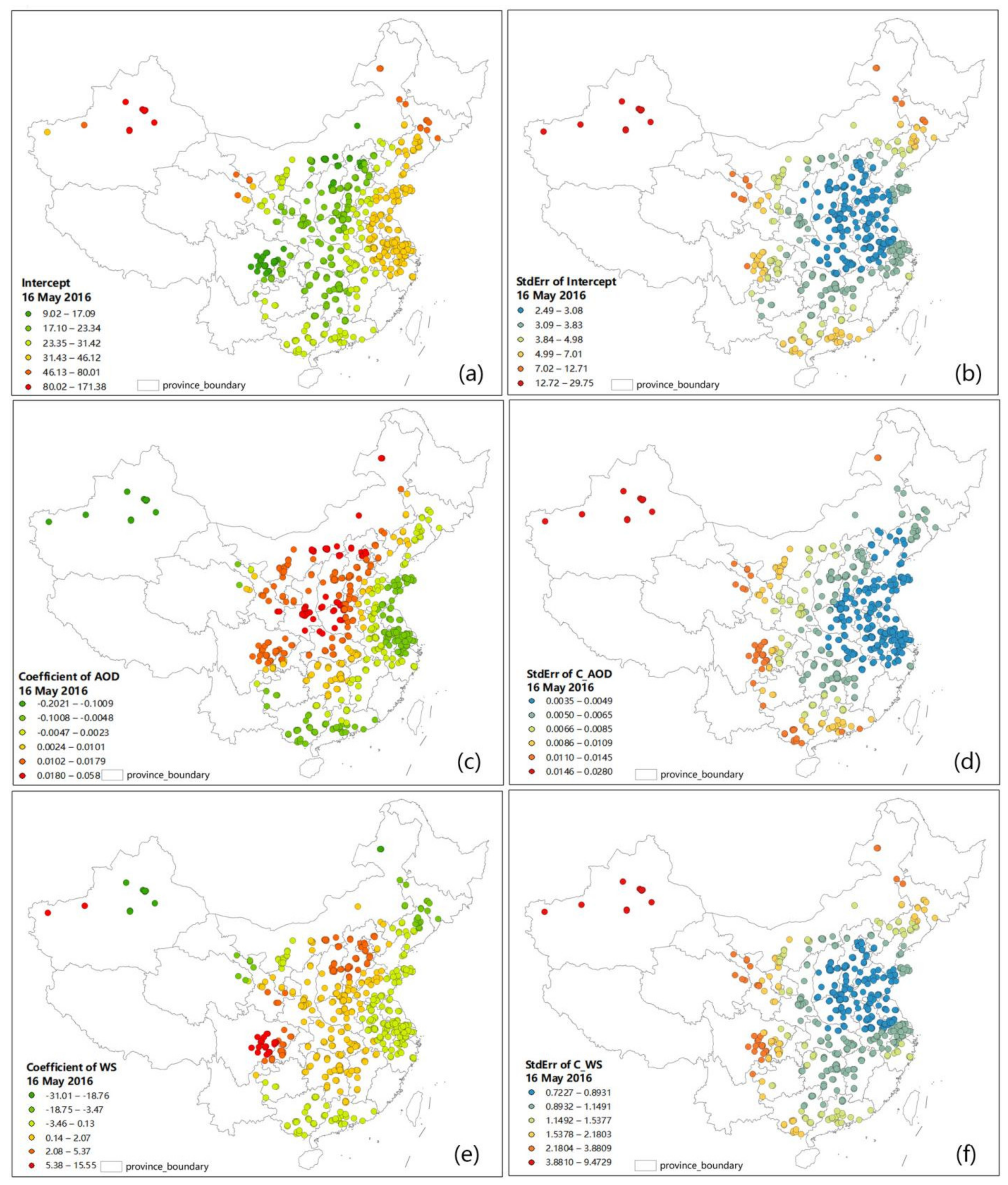
3.1. Analysis of TSAM Model Structure

Based on the framework of the TSAM model [22], 972 daily models were successfully constructed from 1 January 2013 to 31 December 2016. Additionally, the remaining days could not be modeled owing to the lack of sufficient samples. The modeling results demonstrated that AOD was the key variable with the highest rank among all the input parameters. The meteorological variables (wind speed, relative humidity, and precipitation) and land-use variables (e.g., percentage of built-up, forest, and grass) also exhibited high ranks. Other input parameters were relatively less used.
The spatial distributions of the intercept, variable coefficient, and corresponding standard error of the daily fitting model (e.g., 16 May 2016) are shown in Figure 2, presenting significant spatial aggregation. Intercepts ranged from 9.02 to 171.38, with a mean value of 29.79. The coefficient of AOD ranged from −0.2021 to 0.0058, and wind speed ranged from −31.08 to 15.55. A positive value of the variable coefficient indicated that it played a positive effect on PM2.5, and vice versa. The standard error of the intercept ranged from 2.49 to 29.75. Standard errors of the AOD coefficient ranged from 0.0035 to 0.028, and the values of wind speed ranged from 0.7227 to 9.4729. The standard error of coefficients, which measured the reliability of each coefficient estimate, were relatively lower than values of coefficients. At the same time, the residual standard deviations of the TSAM model in the modeling day ranged from −2.66 to 4.84; 97.76% of the modeling samples had residual standard deviations between −2.5 and 2.5.

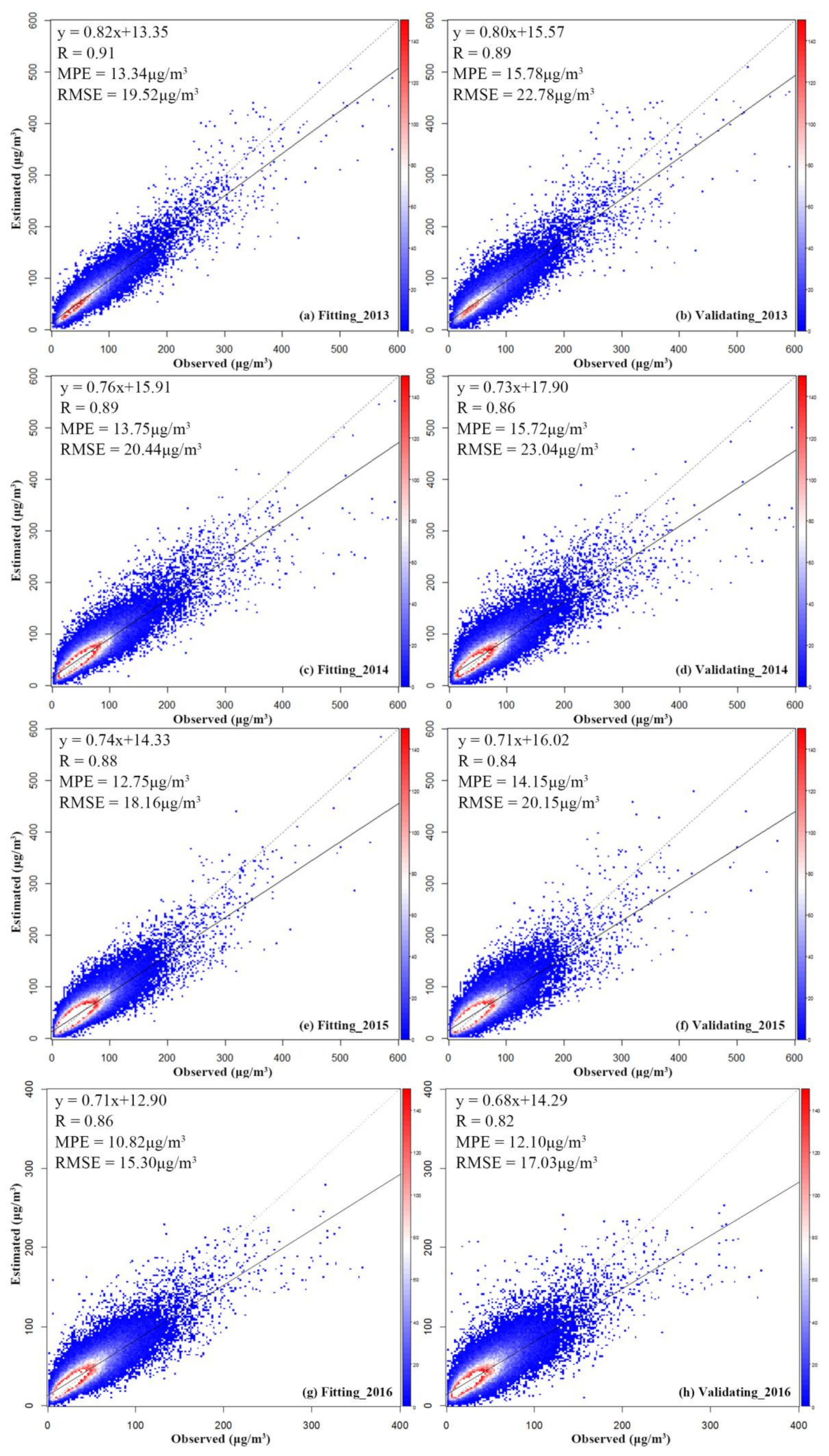
3.2. Fitting and Validation of TSAM Models

Figure 3 demonstrates annual scatter plots of TSAM model fitting and validation from 2013 to 2016. The correlation coefficients of TSAM fitting were 0.91, 0.89, 0.88, and 0.86 for 2013, 2014, 2015, and 2016, respectively. Correspondingly, the values were 0.89, 0.86, 0.84, and 0.82 for cross-validation for each year. Additionally, MPEs of fitting ranged from 10.82 to 13.34 μg/m3, and the values of validation ranged from 12.10 to 15.78 μg/m3. These indicators showed that the model exhibited good performance to simulate the relationship between PM2.5 and explanatory variables.
According to Table 1, the RMSEs and MPEs of TSAM fitting and cross-validation were generally the maximum in winter and the minimum in summer. The maximum RMSEs of fitting and cross-validation were 18.23 and 20.48 μg/m3, 15.86 and 17.33 μg/m3, 15.46 and 16.68 μg/m3, and 16.52 and 17.75 μg/m3 in winter for 2013, 2014, 2015, and 2016, respectively. The corresponding minimum values were 12.97 and 14.92 μg/m3, 12.99 and 14.53 μg/m3, 11.46 and 12.59 μg/m3, and 10.07 and 11.27 μg/m3 in summer. These results were also echoed by the indicators of RPEs and RMPEs.

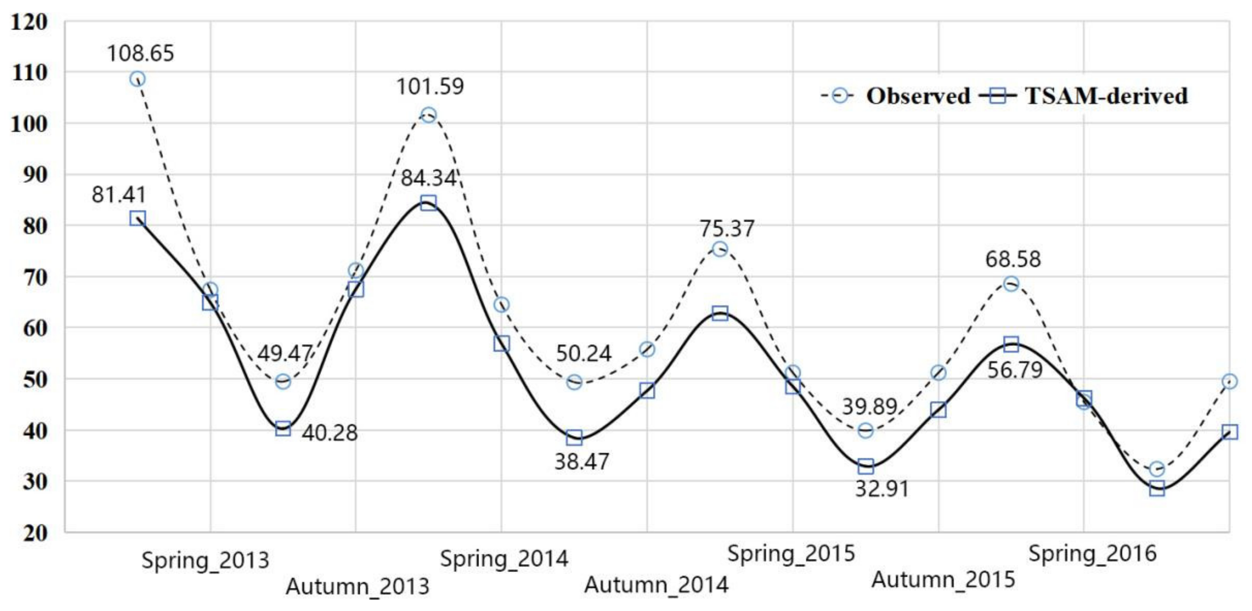
3.3. Temporal Variations in Observed and TSAM-Derived PM2.5

Figure 4 shows the seasonal average values of TSAM-derived and observed PM2.5. Overall, TSAM-derived PM2.5 concentrations were lower than in situ observed values. National annual means of TSAM-derived and site-based PM2.5 both showed a declining trend from 2013 to 2016. They decreased from 64.80 to 43.46 μg/m3 and 74.76 to 50.23 μg/m3, respectively. PM2.5 concentrations demonstrated a significant seasonal regularity with the highest in winter and the lowest in summer. Winter was the season with the worst air quality, with TSAM-derived PM2.5 values of 84.34, 62.82, 56.79, and 69.18 μg/m3 in 2013, 2014, 2015, and 2016, respectively. This could be due to poor pollution diffusion conditions, such as the low temperature and decreases in boundary layer height. In contrast, summer was the cleanest season, with the TSAM-derived values of 40.28, 38.47, 32.91, and 28.59 μg/m3, respectively. The monthly mean values also demonstrated significant periodic features. The highest monthly means of PM2.5 appeared in January, and the lowest appeared in June, July, and August, for every year during the study period.

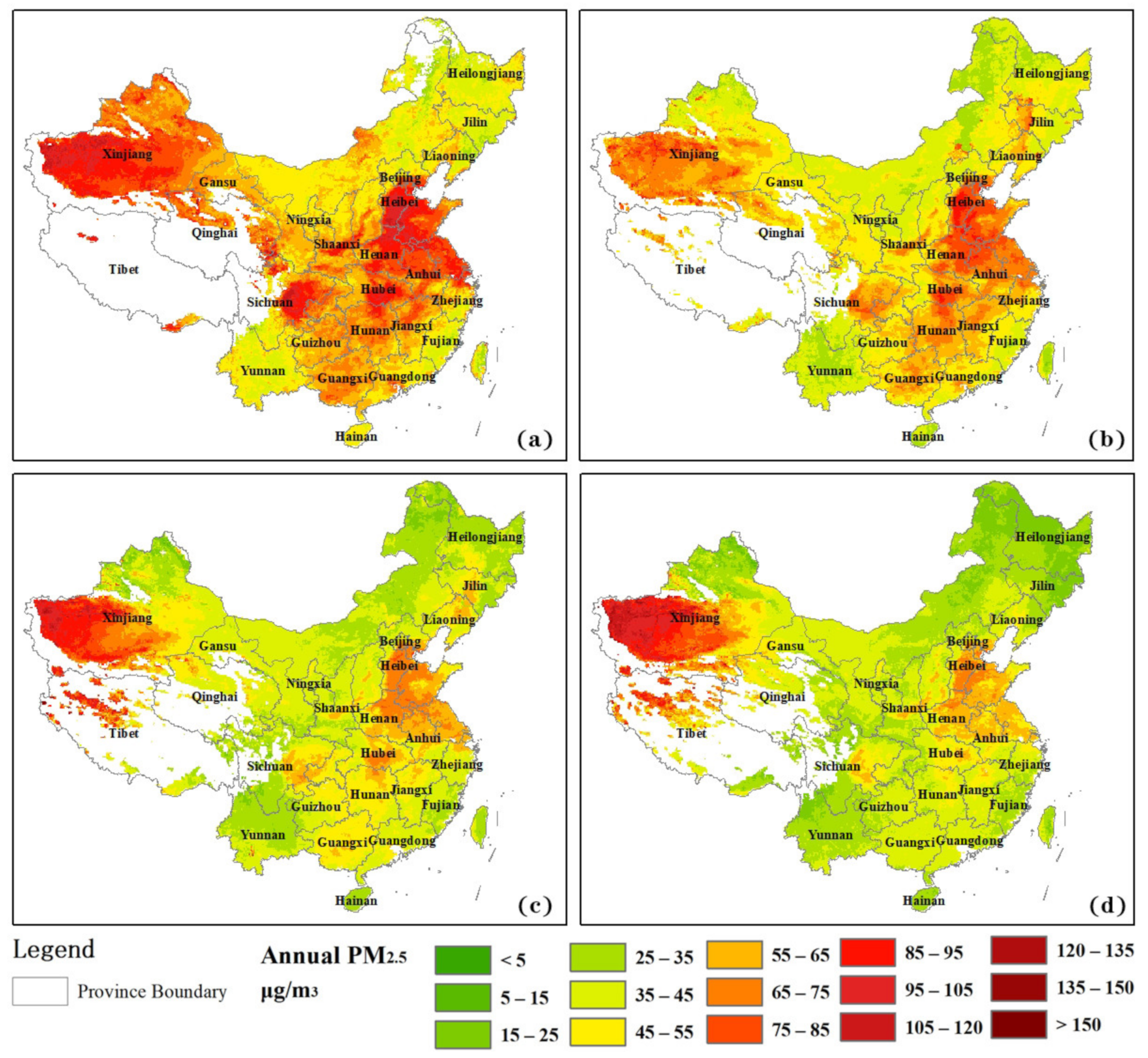
3.4. Spatial Variations in TSAM-Derived PM2.5

Figure 5 shows the spatial distributions of TSAM-derived annual means over mainland China from 2013 to 2016. The blank regions in Figure 5 mean that there were no available annual mean values of TSAM-derived PM2.5, which was due to the missing satellite AOD with the influences of cloud or surface conditions (e.g., ice, snow, etc.). In Figure 5, PM2.5 exhibits significant spatial aggregation. Overall, heavily PM2.5-polluted areas were centrally located in the north plain, center eastern part, the Sichuan Basin, and the Tarim Basin. The Beijing–Tianjin–Hebei urban agglomeration (BTH) was one of the most heavily polluted regions, with annual PM2.5 levels ranging from 45 μg/m3 to 105 μg/m3. Meanwhile, the Shandong Peninsula urban agglomeration and the Chengdu–Chongqing metropolitan area also had non-ignorable levels of PM2.5 pollution, with annual means around 45~95 μg/m3. The spatial distributions of PM2.5 also demonstrated obvious heterogeneous characteristics. Specifically, there were significant differences in PM2.5 between the areas north and south of the Yangtze River; generally, the former levels were higher than the latter. At the same time, there were also clear differences within the same administrative region. For Beijing, the values of PM2.5 ranged from 40 to 70 μg/m3 in 2016. In terms of the spatial distribution, areas with high concentrations (Dongcheng, Xicheng, Chaoyang District, etc.) were located in the centers of the cities, and areas with low concentrations were located towards the north-west, such as Yanqing, Miyun, and Huairou District. Additionally, according to differences in TSAM-derived PM2.5 between 2013 and 2016, over 85% of areas exhibited declines greater than 10 μg/m3 in the study area. The decline in PM2.5 ranged from 10 to 30 μg/m3. The Chengdu–Chongqing metropolitan region also exhibited a strong decline in PM2.5 levels, with average decreases of about 15 to 30 μg/m3.

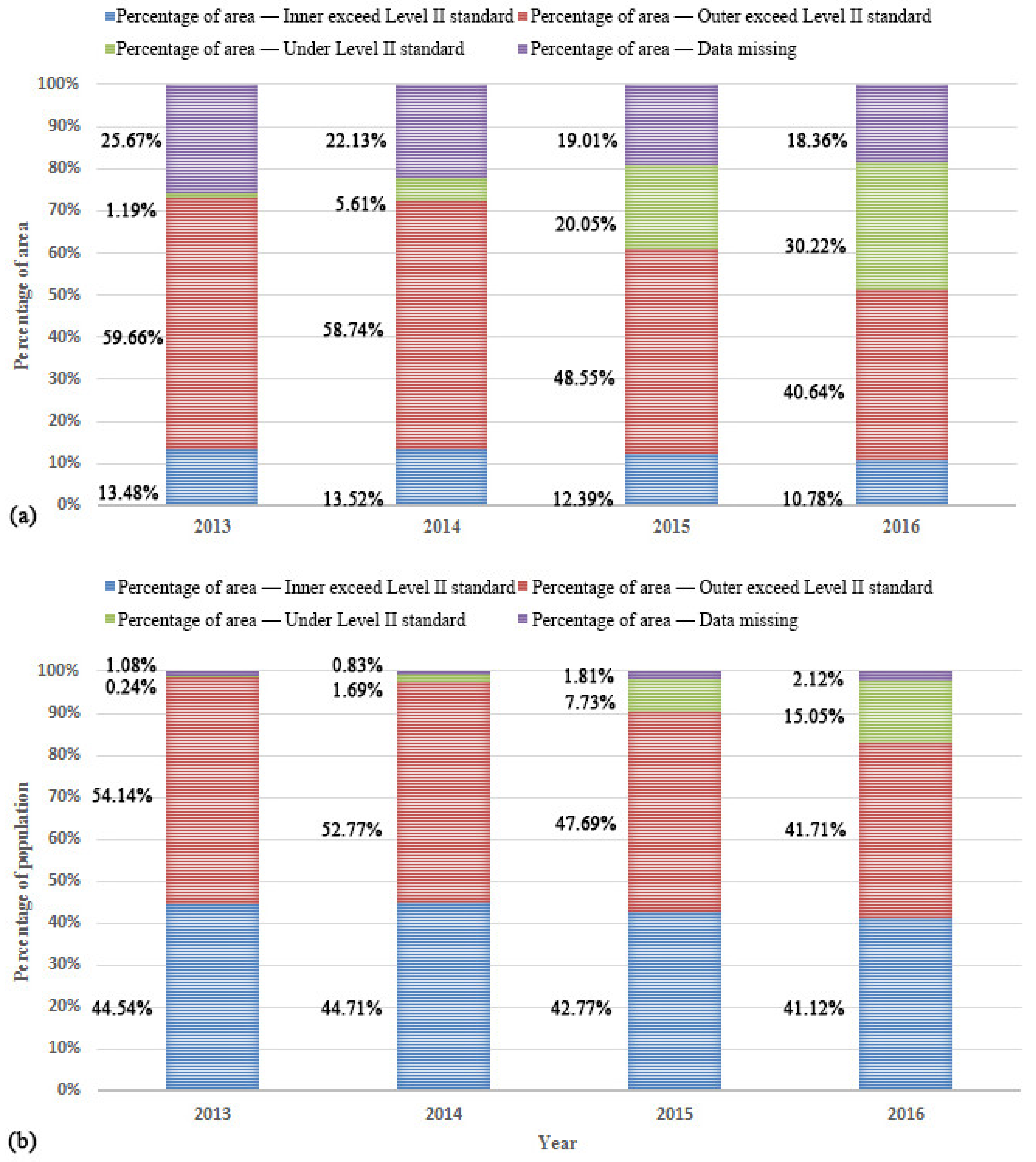
3.5. PM2.5 Variation Analysis Based on Percentage of Area and Population

Summaries of the percentage of area and population exceeding and under air quality Level II standard (annual mean PM2.5 concentration lower than 35 μg/m3) based on TSAM-derived PM2.5 are shown in Figure 6. As Figure 6a shows, 73.14%, 72.26%, 60.94%, and 51.42% of areas suffered annual PM2.5 levels over the Level II standard for 2013, 2014, 2015, and 2016, respectively. The areas with clear air quality (the annual mean of PM2.5 lower than 35 μg/m3) were increased from 1.19% to 30.22%. Correspondingly, in Figure 6b, 98.68%, 97.48%, 90.46%, and 82.83% of the population lived in environments with annual mean concentrations higher than the Level II standard for 2013, 2014, 2015, and 2016, respectively. The proportion of the population who lived in an environment with PM2.5 levels lower than the Level II standard increased by 14.81%.

3.6. Comparison between Observed and Population-Weighted PM2.5 Values for Key Regions

The national population-weighted PM2.5 values decreased from 71.99 μg/m3 to 48.04 μg/m3, with a decrement of 33.27%. To compare the differences among observed and population-weighted PM2.5, Table 2 demonstrates the concentrations in 13 Key Regions for 2013 and 2016. PM2.5 concentrations in the Key Regions exhibited similar declining trends and different magnitudes based on two kinds of values. Eight out of thirteen regions had a decline in observed PM2.5 over 20 μg/m3 from 2013 to 2016. Specifically, the decline in observed PM2.5 levels in Wuhan region was 45.19 μg/m3, which was the highest among the 13 Key Regions from 2013 to 2016. In contrast, the decline in Gansu–Ningxia was only 3.94 μg/m3, which was the lowest. The decline in population-weighted PM2.5 in Urumqi, Xinjiang, with a value of 39.05 μg/m3, was the highest among the 13 Key Regions. The central and northern areas of Shanxi had a 9.79 μg/m3 decline in population-weighted PM2.5.

4. Discussion

This study estimated the spatial–temporal distributions of satellite-derived PM2.5 in four consecutive years from January 2013 to December 2016 in mainland China. Indicators R2 and RMSE of the TSAM model were 0.80 and 22.78 μg/m3, which showed better performances compared to the research of Ma et al. (R2 = 0.79, RMSE = 27.42 μg/m3) [37]. Li et al. proposed a national-scale generalized regression neural network (GRNN) model [38], to simulate PM2.5 in the period from February 2013 to December 2014. This model showed good performance, with fitting R = 0.895 and cross-validated R = 0.816 during the study period. In comparison, our model showed a slight improvement with the fitting R (0.91~0.89) and cross-validating R (0.89~0.86) during the same study period and in the same area. The advantages of TSAM proved that taking the temporal variations and magnitude of predictors into consideration in the modeling process could improve the prediction capability of a statistical model.
To assess the model uncertainty of TSAM, statistic results of standard errors of different variable combinations for modeling samples on 16 May 2016 are demonstrated in Table S1. Among 65 variable combinations, the minimum, lower quartile, average, upper quartile, and maximum values of the model with AOD as the only explanatory variable were 0.23, 8.47, 8.48, 8.62, and 8.66 μg/m3, respectively. With the addition of meteorological factors in explanatory variables, not all of these factors could reduce the model uncertainty. The z-score of temperature with the spatial autocorrelation (Moran’s I) test was 37.51 Standard Deviations (std), which indicated that it had a significant spatial autocorrelation, and then it was not included in the TSAM model. Among the meteorological factors, only wind speed was added in the list of explanatory variables, and the model uncertainty decreased. This means that the wind speed, which could change the dispersion condition, had a significant effect on PM2.5 variations. The addition of the precipitation variable did not reduce the standard error, which could be due to its transient effects on PM2.5 such as the hourly scale, but the TSAM model in this study was developed with the daily scale. With the quantitative comparison of the standard error of 65 variable combinations, we found the model performance did not necessarily get better as the variables increased. The screening of explanatory variables is an important process for PM2.5 simulation. With the screening, the explanatory variables of the TSAM model in this study day were defined as AOD, wind speed, percentage of forest, and percentage of water.
Both TSAM-derived and observed PM2.5 values exhibited a significant decline during the study period, which proved that implementing air pollution prevention and control policies had a significant effect on improving the air quality. The annual and monthly concentrations of TSAM-derived PM2.5 were lower than those observed for each region. The reasons for this could be that in situ observations revealed PM2.5 levels near the ground monitoring station, which were generally located in urban areas with high PM2.5 pollutant emissions.
TSAM-derived PM2.5 showed a strong signature of seasonal variations, with the highest concentrations in winter and the lowest concentrations in summer, and intermediate ranges in spring and autumn during the study period. Winter heating could be the main cause of the high PM2.5 levels, especially in northern and western China. During seasons when more heating was needed, the pollutant emissions sharply increased, and the PM2.5 concentration rose correspondingly. In addition to free heating policies, the Spring Festival, which lasts from January to February, could be another key cause of seriously increased pollution in winter. During the Spring Festival, people set off large quantities of fireworks in celebration. Thus, PM2.5 concentrations sharply increase in January, which is the most polluted month of the year. Meanwhile, there were some areas, especially in northern China, which suffered serious PM2.5 pollution in spring (from March to May) due to dust storms. The percentage of polluted area increased by 29.03%, whereas the percentage of the population living under the Level II standard only increased by 14.81% during the study period. The difference between the percentages of area and population is attributable to the spatial heterogeneity of population distribution, i.e., some regions had relatively low population density and their air quality had been improved from 2013 to 2016. Moreover, the spatial continuity of air pollutant concentrations may be another reason for this result. This means that the implementation of air pollution prevention and control measures could not only directly improve local air quality, but also affect surrounding air quality at the same time.
The population-weighted PM2.5 concentrations of the 13 Key Regions showed declines of more than 10 μg/m3 from 2013 to 2016, except for the central and northern regions of Shanxi. Correspondingly, the declining proportion in population-weighted PM2.5 was more than 15%. The declines in in situ observations of PM2.5 ranged from 3.94 to 45.19 μg/m3 for the 13 Key Regions. Ground-level monitoring measurements could only represent air pollutant concentrations in limited ranges around the stations; however, population-weighted PM2.5 not only considered the wider spatial range but also took the population into consideration, which could better represent the health threats of air pollutants compared with merely in situ observations.
The population-weighted PM2.5 with a spatial resolution of 10 km could offer support for the large-scale analysis of air pollutant variations, but is relatively coarse to reflect features of the local variation in PM2.5. Urban air quality has clear spatial differentiations among small intra-urban scenarios. The limitations of operational satellite product could be improved with the development of a satellite retrieval algorithm. Moreover, the temporal variation analyses of PM2.5 were implemented under relatively long-term temporal scales, such as monthly, seasonal, and annual. Long-term temporal scales could be used to represent the global trends in PM2.5 variation, as well as to capture the short-term variation. With the development of stationary satellites, the temporal scale of satellite products can be improved to hourly with continuous sequences, which would capture dynamic variation in air pollutant levels. Additionally, this would greatly enhance the significance of satellite-based modeling and estimations of PM2.5 for real-time air pollution exposure assessments. More importantly, satellite data coverage could cause misunderstandings in annual mean difference analyses. For example, the value for Central Liaoning exhibited an increasing trend from 2013 to 2014 due to the low coverage of AOD systems in the winter of 2013 and a relatively high coverage in the winter of 2014. Thus, new algorithms for remedying the coverage of satellite-based AOD values are also urgently required for contemporary PM2.5 modeling and estimation.

5. Conclusions

This study developed a national daily TSAM model for PM2.5 concentration prediction using variables of satellite AOD, meteorology, land-use, etc., from January 2013 to December 2016. The TSAM model demonstrated good performance by taking timely variations and magnitudes of predictors into consideration in the modeling process. The TSAM-derived PM2.5 could represent a large spatial range and reported consecutive spatial variations, which complements site-based observations of PM2.5. Both in situ observations and TSAM-derived concentrations proved that the air quality showed great improvements from 2013 to 2016, due to the implementation of air pollution prevention and control policies. According to the air quality Level II standard, the majority of the population was subjected to PM2.5 concentrations above this standard. The population based on the satellite-derived concentrations represents a complementary indicator to analyze the concentrations of air pollutants.

Supplementary Materials

The following supporting information can be downloaded at: https://www.mdpi.com/article/10.3390/rs14143381/s1, Figures S1–S12: Time average maps of input variables. Table S1: Statistic of standard error of TSAM with different variable combination.

Author Contributions

X.F. performed the experiments and drafted the manuscript text; S.L. participated in experimental designs, data analyses, and manuscript revisions; L.X. helped with data collection and processing; B.Z. supervised and designed the research work. All authors have read and agreed to the published version of the manuscript.

Funding

This research was funded by the Natural Science Foundation of Hunan Province (Grant No. 2021JJ40022), the Research Foundation of Education Bureau of Hunan Province, China (Grant No. 19B107), and the National Natural Science Foundation of China (41871317).

Data Availability Statement

Hourly ground PM2.5 concentrations were collected from the official database of the China Environmental Monitoring Center (CEMC) (http://www.cnemc.cn/) (accessed on 18 May 2022). The Level 2 C6 MODIS AOD of Terra (equatorial crossing time at 10:30 a.m) and Aqua (equatorial crossing time at 13:30 p.m) with the spatial resolution of 10 km were collected from the Level-1 and Atmosphere Archive and Distribution System (LAADS web, on https://ladsweb.nascom.nasa.gov/search) (accessed on 18 May 2022). Population raster data were provided by the Data Center for Resources and Environmental Sciences, Chinese Academy of Sciences (RESDC, on http://www.resdc.cn) (accessed on 18 May 2022). Land use data and traffic network data were collected from the Geographical Information Monitoring Cloud Platform (GIMCP, on http://www.dsac.cn/) (accessed on 18 May 2022). Meteorological data were collected from the China Meteorological Data Sharing Service System (CMDSS, on http://www.nmic.cn/) (accessed on 18 May 2022). Shuttle Radar Topography Mission (SRTM), with a spatial resolution of 90 m, was collected from United States Geological Survey (USGS, on https://gisgeography.com/usgs-earth-explorer-download-free-landsat-imagery/) (accessed on 18 May 2022).

Conflicts of Interest

The authors declare no conflict of interest.

References

  1. Emmanuela, G.; Ashkan, A.; Amanuel, A.A.; Kalkidan, H.A.; Cristiana, A.; Kaja, M.A.; Foad, A.; Abdishakur, M.A.; Semaw, F.A.; Victor, A. Global, regional, and national comparative risk assessment of 84 behavioural, environmental and occupational, and metabolic risks or clusters of risks, 1990–2016: A systematic analysis for the Global Burden of Disease Study 2016. Lancet 2017, 390, 1345–1422. [Google Scholar]
  2. Lelieveld, J.; Evans, J.S.; Fnais, M.; Giannadaki, D.; Pozzer, A.A. The contribution of outdoor air pollution sources to premature mortality on a global scale. Nature 2017, 525, 367–371. [Google Scholar] [CrossRef] [PubMed]
  3. Yin, P.; Brauer, M.; Cohen, A.; Burnett, R.T.; Liu, J.; Liu, Y.; Liang, R.; Wang, W.; Qi, J.; Wang, L.; et al. Long-term fine particulate matter exposure and nonaccidental and cause-specific mortality in a large national cohort of Chinese men. Environ. Health Perspect. 2017, 125, 117002. [Google Scholar] [CrossRef] [PubMed]
  4. Shen, M.; Gu, X.; Li, S.; Yu, Y.; Zou, B.; Chen, X. Exposure to black carbon is associated with symptoms of depression: A retrospective cohort study in college students. Environ. Int. 2021, 157, 106870. [Google Scholar] [CrossRef]
  5. Varotsos, C.; Tzanis, C.; Cracknell, A. The enhanced deterioration of the cultural heritage monuments due to air pollution. Environ. Sci. Pollut. Res. 2009, 16, 590–592. [Google Scholar] [CrossRef]
  6. Van Donkelaar, A.; Martin, R.V.; Brauer, M.; Kahn, R.; Levy, R.; Verduzco, C.; Villeneuve, P.J. Global estimates of ambient fine particulate matter concentrations from satellite-based aerosol optical depth: Development and application. Enivron. Health Persp. 2010, 118, 847. [Google Scholar] [CrossRef] [Green Version]
  7. Zhao, P.; Zhang, X.; Xu, X.; Zhao, X. Long-term visibility trends and characteristics in the region of Beijing, Tianjin, and Hebei, China. Atmos. Res. 2011, 101, 711–718. [Google Scholar] [CrossRef]
  8. Brimblecombe, P. Visibility Driven Perception and Regulation of Air Pollution in Hong Kong, 1968–2020. Environments 2021, 8, 51. [Google Scholar] [CrossRef]
  9. Liu, Z.; Qi, Z.; Ni, X.; Dong, M.; Ma, M.; Xue, W.; Zhang, Q.; Wang, J. How to apply O3 and PM2.5 collaborative control to practical management in China: A study based on meta-analysis and machine learning. Sci. Total Environ. 2021, 772, 145392. [Google Scholar] [CrossRef]
  10. Liu, Z.; Xue, W.; Ni, X.; Qi, Z.; Zhang, Q.; Wang, J. Fund gap to high air quality in China: A cost evaluation for PM2.5 abatement based on the Air Pollution Prevention and control Action Plan. J. Clean. Prod. 2021, 319, 128715. [Google Scholar] [CrossRef]
  11. Shi, W.; Bi, J.; Liu, R.; Liu, M.; Ma, Z. Decrease in the chronic health effects from PM2.5 during the 13th Five-Year Plan in China: Impacts of air pollution control policies. J. Clean. Prod. 2021, 317, 128433. [Google Scholar] [CrossRef]
  12. Van Donkelaar, A.; Martin, R.V.; Spurr, R.J.D.; Burnett, R.T. High-resolution satellite-derived PM2.5 from optimal estimation and geographically weighted regression over north America. Environ. Sci. Tech. 2015, 49, 10482–10491. [Google Scholar] [CrossRef]
  13. Rohde, R.A.; Muller, R.A. Air pollution in China: Mapping of concentrations and sources. PLoS ONE. 2015, 10, e0135749. [Google Scholar] [CrossRef]
  14. Zou, B.; Luo, Y.; Wan, N.; Zheng, Z.; Sternberg, T.; Liao, Y. Performance comparison of LUR and OK in PM2.5 concentration mapping: A multidimensional perspective. Sci. Rep. 2015, 5, 8698. [Google Scholar] [CrossRef] [Green Version]
  15. Yang, Y.; Christakos, G. Spatiotemporal characterization of ambient PM2.5 concentration in Shandong province (China). Environ. Sci. Tech. 2015, 49, 13431–13438. [Google Scholar] [CrossRef]
  16. Di, Q.; Kloog, I.; Koutrakis, P.; Lyapustin, A.; Wang, Y.; Schwartz, J. Assessing PM2.5 exposures with high spatiotemporal resolution across the continental United States. Envion. Sci. Tech. 2016, 50, 4712–4721. [Google Scholar] [CrossRef] [Green Version]
  17. Lee, H.J.; Chatfield, R.B.; Strawa, A.W. Enhancing the applicability of satellite remote sensing for PM2.5 estimation using MODIS deep blue AOD and land use regression in California, United States. Environ. Sci. Tech. 2016, 50, 6546–6555. [Google Scholar] [CrossRef]
  18. Cracknell, A.P.; Varotsos, C.A. New aspects of global climate-dynamics research and remote sensing. Int. J. Remote Sens. 2011, 32, 579–600. [Google Scholar] [CrossRef]
  19. Kahn, R.; Banerjee, P.; McDonald, D.; Diner, D.J. Sensitivity of multiangle imaging to aerosol optical depth, and to pure-particle size distribution and composition over ocean. J. Geophys. Res. Atmos. 1998, 103, 32195–32213. [Google Scholar] [CrossRef]
  20. Kahn, R.; Banerjee, P.; McDonald, D. Sensitivity of multiangle imaging to natural mixtures of aerosols over ocean. J. Geophys. Res. Atmos. 2001, 106, 18219–18238. [Google Scholar] [CrossRef] [Green Version]
  21. Ma, Z.; Hu, X.; Huang, L.; Bi, J.; Liu, Y. Estimating ground-level PM2.5 in China using satellite remote sensing. Environ. Sci. Tech. 2014, 48, 7436–7444. [Google Scholar] [CrossRef]
  22. Fang, X.; Zou, B.; Liu, X.; Sternberg, T.; Zhai, L. Satellite-based ground PM2.5 estimation using timely structure adaptive modeling. Remote Sens. Enivron. 2016, 186, 152–163. [Google Scholar] [CrossRef]
  23. Wang, J.; Christopher, S.A. Intercomparison between satellite-derived ground-level fine aerosol optical thickness and PM2.5 mass: Implications for air quality studies. Geophys. Res. Lett. 2003, 30, 2067–2283. [Google Scholar] [CrossRef]
  24. Liu, Y.; Sarnat, J.A.; Kilaru, V.; Jacob, D.J.; Koutrakis, P. Estimating ground-level PM2.5 in the eastern United States using satellite remote sensing. Environ. Sci. Tech. 2005, 39, 3269–3278. [Google Scholar] [CrossRef] [Green Version]
  25. Zou, B.; Pu, Q.; Bilal, M.; Weng, Q.; Zhai, L.; Nichol, J.E. High-resolution satellite mapping of fine particulates based on geographically weighted regression. IEEE Geosci. Remote Sens. Lett. 2016, 13, 495–499. [Google Scholar] [CrossRef]
  26. Ma, Z.; Liu, Y.; Zhao, Q.; Liu, M.; Zhou, Y.; Bi, J. Satellite-derived high resolution PM2.5 concentrations in Yangtze River Delta region of China using improved linear mixed effects model. Atmos. Environ. 2016, 133, 156–164. [Google Scholar] [CrossRef]
  27. Pu, Q.; Yoo, E. Spatio-temporal modeling of PM2.5 concentrations with missing data problem: A case study in Beijing, China. Int. J. Geogr. Inf. Sci. 2020, 34, 423–447. [Google Scholar] [CrossRef]
  28. Zou, B.; Wang, M.; Wan, N.; Wilson, J.G.; Fang, X.; Tang, Y. Spatial modeling of PM2.5 concentrations with a multifactorial radial basis function neural network. Environ. Sci. Pollut. Res. 2015, 22, 10395–10404. [Google Scholar] [CrossRef]
  29. Chen, Z.Y.; Zhang, T.-H.; Zhang, R.; Zhu, Z.-M.; Yang, J.; Chen, P.-Y.; Ou, C.-Q.; Guo, Y. Extreme gradient boosting model to estimate PM2.5 concentrations with missing-filled satellite data in China. Atmos. Environ. 2019, 202, 180–189. [Google Scholar] [CrossRef]
  30. Yan, X.; Zang, Z.; Luo, N.; Jiang, Y.; Li, Z. New interpretable deep learning model to monitor real-time PM2.5 concentrations from satellite data. Environ. Int. 2020, 144, 106060. [Google Scholar] [CrossRef]
  31. Hu, H.Y. The distribution of population in China, with statistics and maps. Acta Geograph. Sin. 1935, 2, 33–74. (In Chinese) [Google Scholar] [CrossRef]
  32. Lee, H.J.; Liu, Y.; Coull, B.A.; Schwartz, J.; Koutrakis, P. A novel calibration approach of MODIS AOD data to predict PM2.5 concentrations. Atmos. Chem. Phys. 2011, 11, 7991–8002. [Google Scholar] [CrossRef] [Green Version]
  33. Puttaswamy, S.J.; Nguyen, H.M.; Braverman, A.; Hu, X.; Liu, Y. Statistical data fusion of multi-sensor AOD over the Continental United States. Geocarto. Int. 2014, 29, 48–64. [Google Scholar] [CrossRef]
  34. Tian, J.; Chen, D. A semi-empirical model for predicting hourly ground-level fine particulate matter (PM2.5) concentration in southern Ontario from satellite remote sensing and ground-based meteorological measurements. Remote Sens. Environ. 2010, 114, 221–229. [Google Scholar] [CrossRef]
  35. Rodriguez, J.D.; Perez, A.; Lozano, J.A. Sensitivity analysis of k-fold cross validation in prediction error estimation. IEEE Trans. Pattern Anal. Mach. Intell. 2010, 32, 569–575. [Google Scholar] [CrossRef]
  36. Zou, B.; Zeng, Y.; Zhan, F.B.; Charles, Y.; Liu, X. Performance of kriging and EWPM for relative air pollution exposure risk assessment. Int. J. Environ. Res. 2011, 5, 769–778. [Google Scholar]
  37. Ma, Z.; Hu, X.; Sayer, A.M.; Levy, R.; Zhang, Q.; Xue, Y.; Tong, S.; Bi, J.; Huang, L.; Liu, Y. Satellite-based spatiotemporal trends in PM2.5 concentrations: China, 2004–2013. Environ. Health Perspect. 2016, 124, 184–192. [Google Scholar] [CrossRef] [Green Version]
  38. Li, T.; Shen, H.; Zeng, C.; Yuan, Q.; Zhang, L. Point-surface fusion of station measurements and satellite observations for mapping PM2.5 distribution in China: Methods and assessment. Atmos. Environ. 2017, 152, 477–489. [Google Scholar] [CrossRef] [Green Version]
Figure 1. Study area.
Remotesensing 14 03381 g001
Figure 2. Spatial distribution of coefficient and standard error of TSAM fitting (e.g., 16 May 2016). (a,c,e) show the intercept, coefficient of AOD, and wind speed, respectively. (b,d,f) show the standard errors of the corresponding intercept and coefficient.
Remotesensing 14 03381 g002
Figure 3. Scatter plot of TSAM model fitting and cross-validation from 2013 to 2016. (a,c,e,g) represent the scatter of TSAM fitting for 2013, 2014, 2015, and 2016, respectively. (b,d,f,h) represent validating result. The dotted line represents the 1:1 line and the solid line represents the trend line. The legend represents the density of sample.
Remotesensing 14 03381 g003
Figure 4. Seasonal average values of TSAM-derived and in situ observed PM2.5.
Remotesensing 14 03381 g004
Figure 5. Spatial distributions of TSAM-derived annual means of PM2.5. (ad) correspond to 2013, 2014, 2015, and 2016, respectively.
Remotesensing 14 03381 g005
Figure 6. Statistics of the percentages of area and population over and under air quality Level II standard (annual mean PM2.5 concentration lower than 35 μg/m3). (a) Percentage of area and (b) percentage of population.
Remotesensing 14 03381 g006
Table 1. Statistical indicators of fitting and cross-validation of TSAM modeling at seasonal scale. N represents the sample number and Mean (μg/m3) denotes the mean value of PM2.5 concentrations. The units of the RMSE and MPE are μg/m3.
FittingCross-Validation
YearSeasonNMeanRMSEMPERPERMPERMSEMPERPERMPE
2013Spring645166.8014.5810.5521.04%15.79%16.8212.8425.18%19.22%
Summer713347.5412.979.4527.28%19.87%14.9211.0231.38%23.18%
Autumn11,95870.7916.1612.2522.83%17.31%18.3814.1625.97%20.00%
Winter11,59394.3918.2314.4319.31%15.29%20.4816.4221.69%17.39%
2014Spring16,97261.5614.5711.2523.67%18.27%16.1912.6526.29%20.54%
Summer14,14749.2612.999.9126.37%20.11%14.5311.2429.49%22.83%
Autumn17,57457.2014.5811.1225.50%19.45%16.4212.7028.71%22.21%
Winter18,12369.7315.8612.7122.75%18.22%17.3314.0124.86%20.01%
2015Spring25,11649.3713.3110.4726.96%21.21%14.4111.4229.18%23.14%
Summer20,47538.3111.468.9129.91%23.25%12.599.8632.86%25.72%
Autumn20,85746.8813.2310.3228.22%22.02%14.4311.3830.79%24.28%
Winter11,21258.6815.4612.3226.34%21.00%16.6813.4428.43%22.90%
2016Spring19,32544.9513.1710.2329.29%22.76%14.3911.2932.01%25.12%
Summer19,67331.4310.077.6632.03%24.37%11.278.6435.87%27.49%
Autumn18,22245.2313.1810.2329.13%22.63%14.6011.4632.28%25.34%
Winter559674.8016.5213.4422.09%17.96%17.7514.5923.72%19.51%
Table 2. Observed and population-weighted PM2.5 in Key Regions (unit: μg/m3).
Regions20132016Difference between 2013 and 2016
ExpConObsConExpConObsConExpDiffObsDiff
BTH Delta87.5585.4162.6467.02−24.91−18.39
Wuhan Region86.25104.9555.5759.76−30.68−45.19
Shandong Province85.6897.0160.6260.52−25.06−36.49
Chengdu–Chongqing84.3775.3748.5152.44−35.86−22.93
Shaanxi Guanzhong83.9994.1153.7858.66−30.21−35.45
Yangtze River Delta77.7471.2852.2551.24−25.49−20.04
Changsha–Zhuzhou–Xiangtan74.5877.9048.4154.66−26.17−23.24
Urumqi, Xinjiang72.5971.0033.5431.62−39.05−39.38
Pearl River Delta64.7670.0442.1941.80−22.57−28.24
Gansu–Ningxia60.1453.1242.9849.18−17.16−3.94
Central and northern areas of Shanxi58.6762.7748.8856.96−9.79−5.81
Central Liaoning57.3952.2344.1841.02−13.21−11.21
Straits Fujian47.0942.4335.4533.86−11.64−8.57
ExpCon represents the population-weighted PM2.5 concentration; ObsCon represents the observed PM2.5. ExpDiff is the differences of population-weighted PM2.5 between 2013 and 2016; ObsDiff is the differences of observed PM2.5 between 2013 and 2016.
Publisher’s Note: MDPI stays neutral with regard to jurisdictional claims in published maps and institutional affiliations.

