
Machine Learning Techniques for Phenology Assessment of Sugarcane Using Conjunctive SAR and Optical Data


Abstract
:1. Introduction
2. Materials and Methods
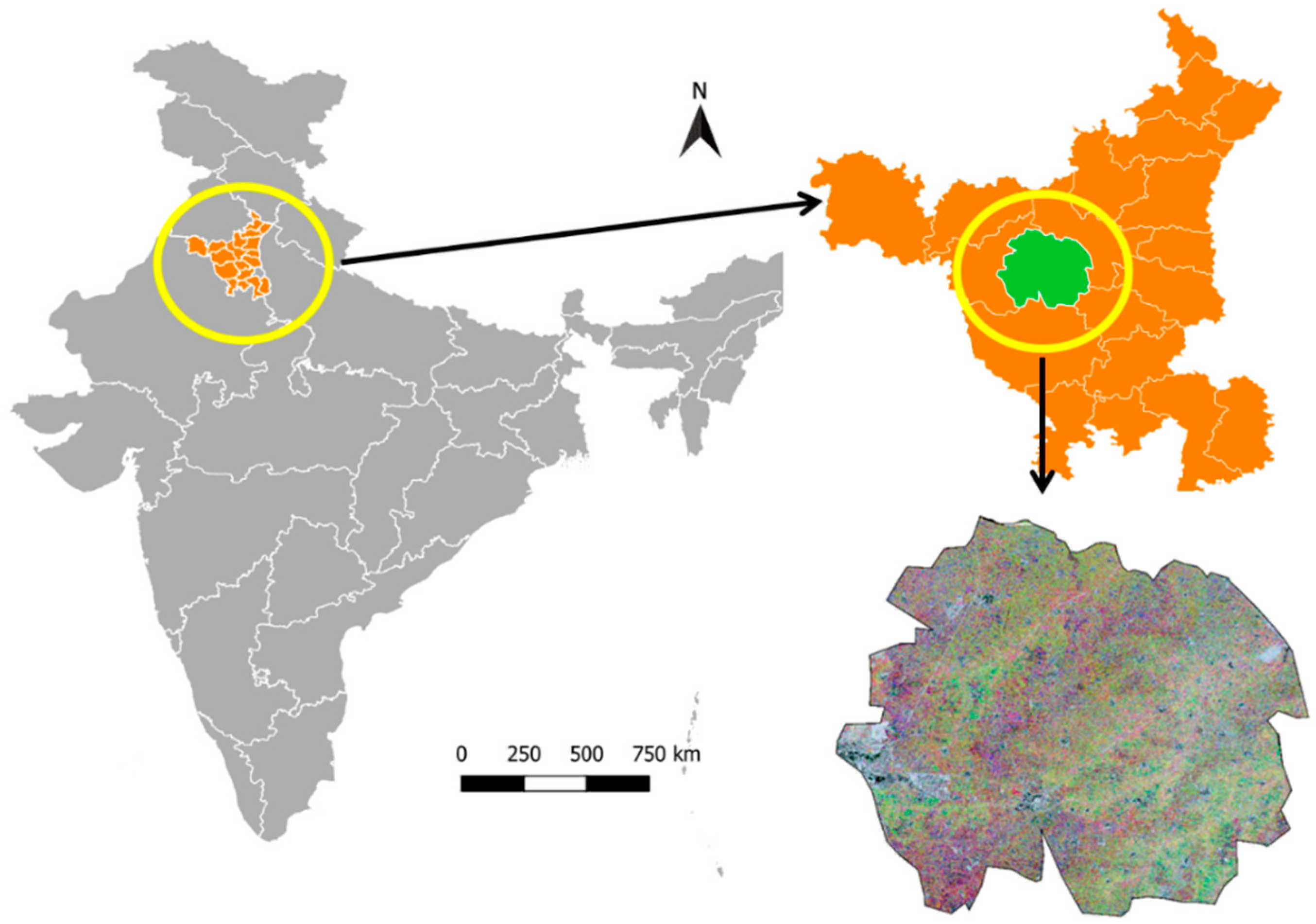
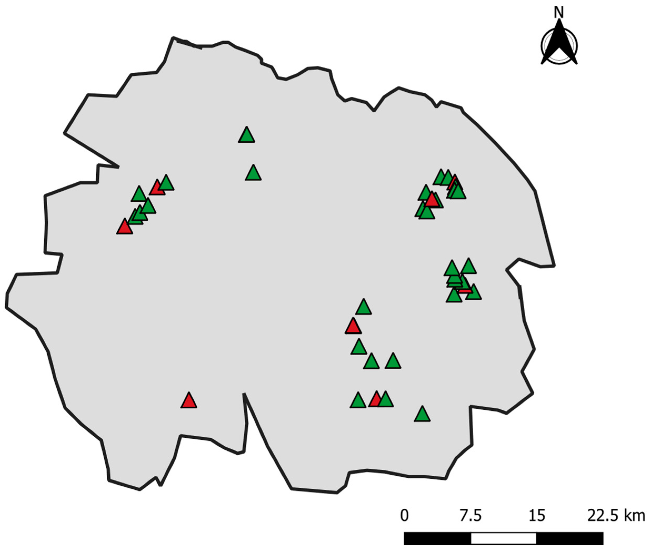
2.1. Study Region
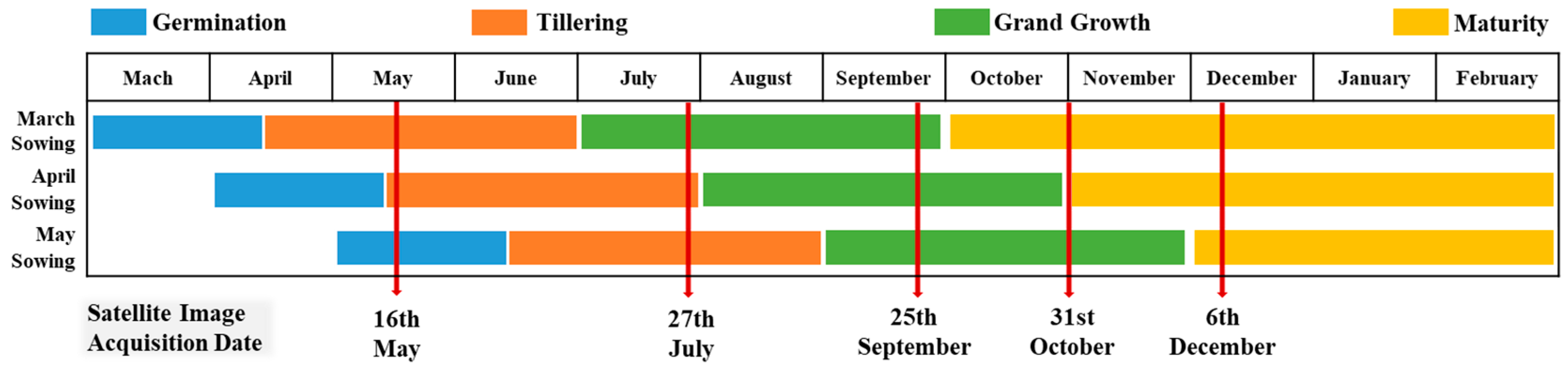
2.2. Datasets
2.2.1. Pre-Processing of SLC Data
2.2.2. Pre-Processing of GRD Data
2.2.3. Pre-Processing of Sentinel-2 Data
2.3. Methods
2.3.1. Logistic Regression
2.3.2. Naïve Bayes
2.3.3. Support Vector Machine Learning
2.3.4. Decision Tree
2.3.5. Random Forest
2.3.6. Neural Network
2.3.7. FRBS (Fuzzy Rule Based Systems)
3. Results
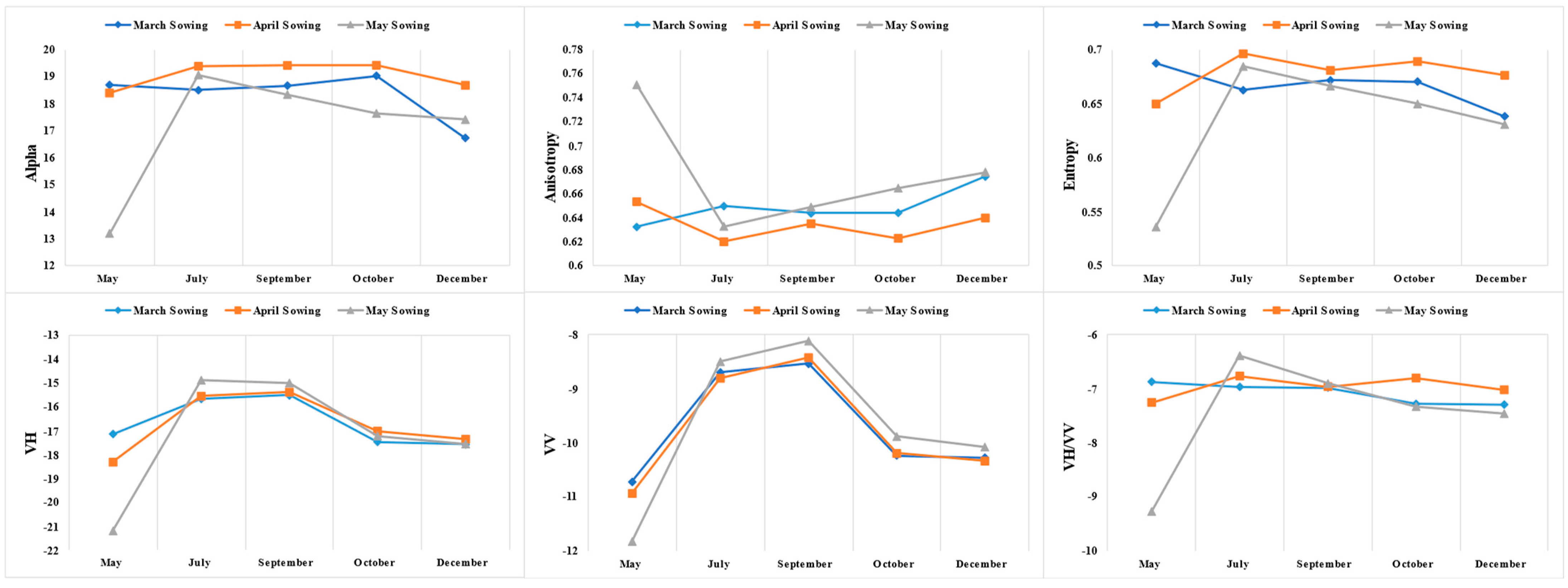
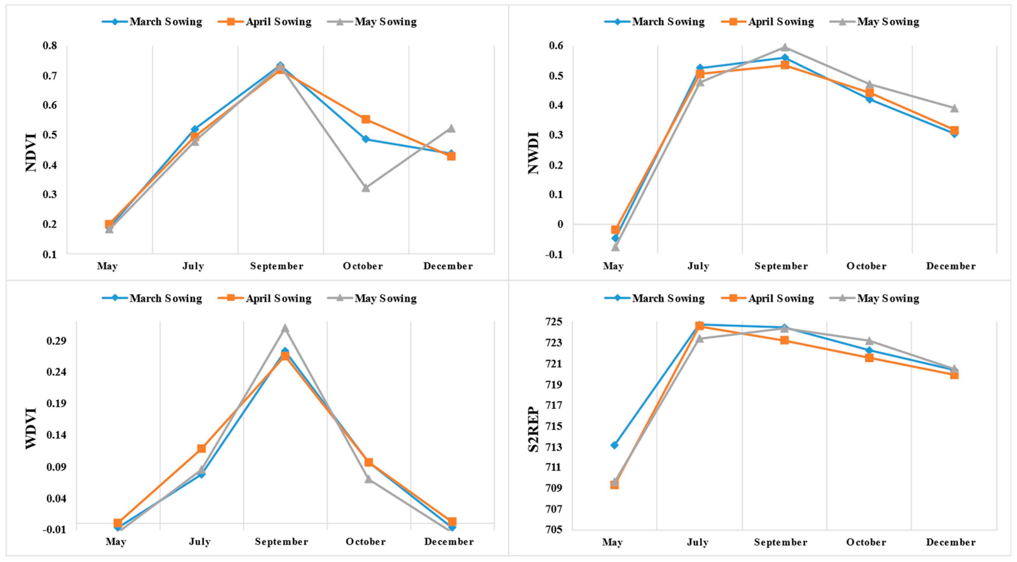
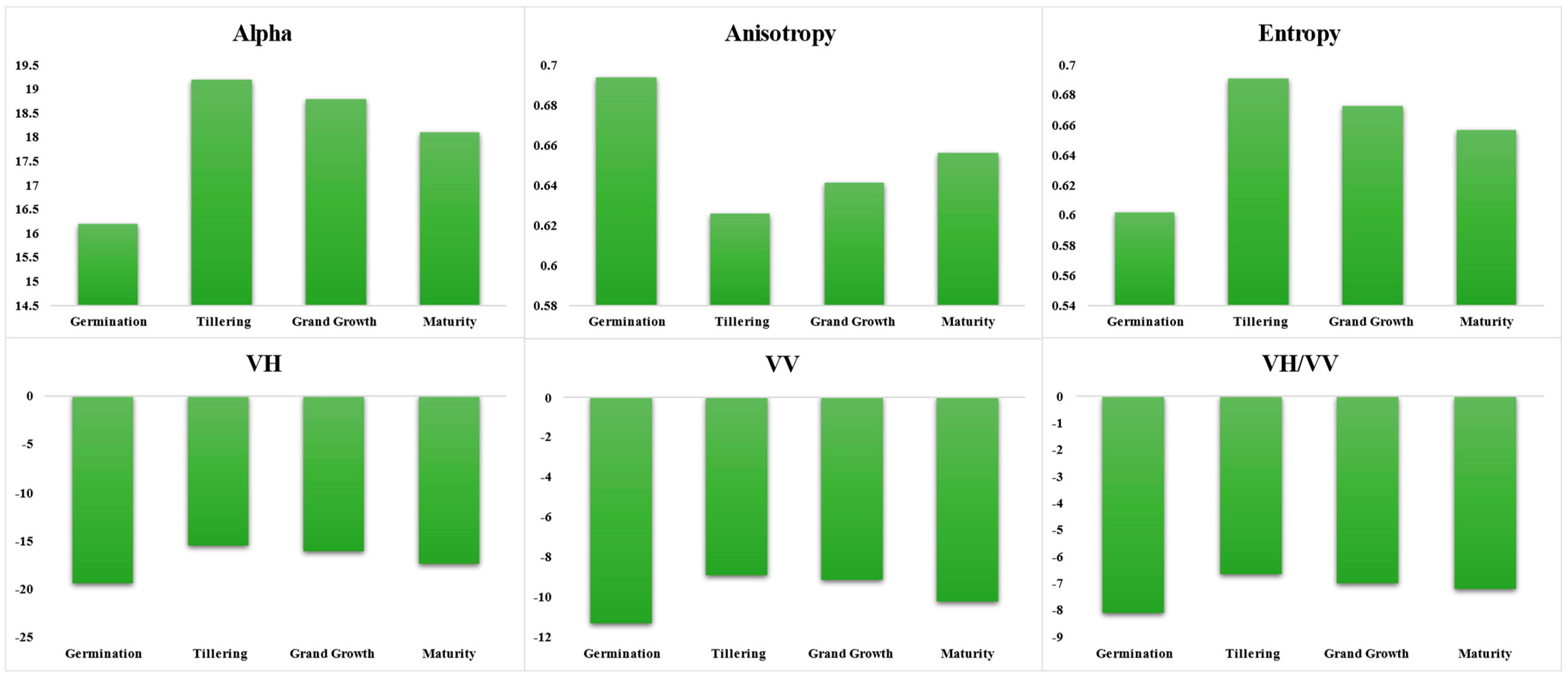
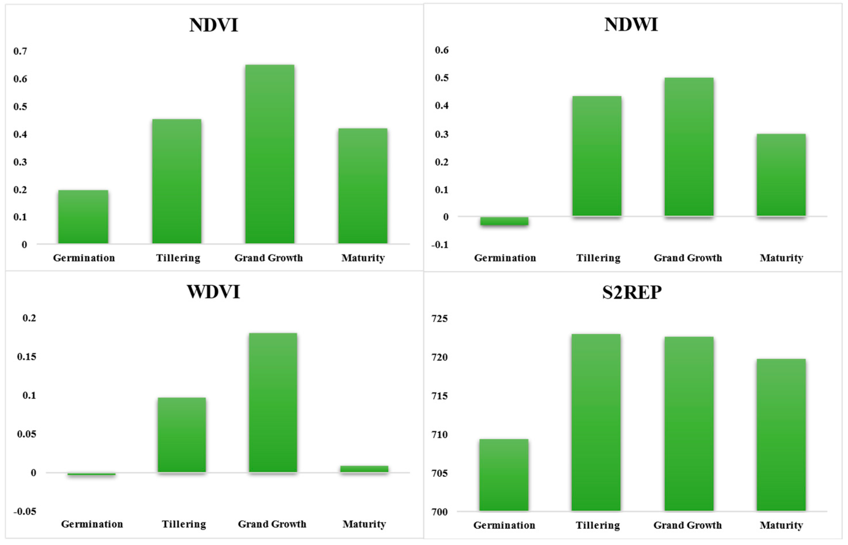
3.1. Temporal Analysis of Sentinel-1 Parameters and Sentinel-2 Indices
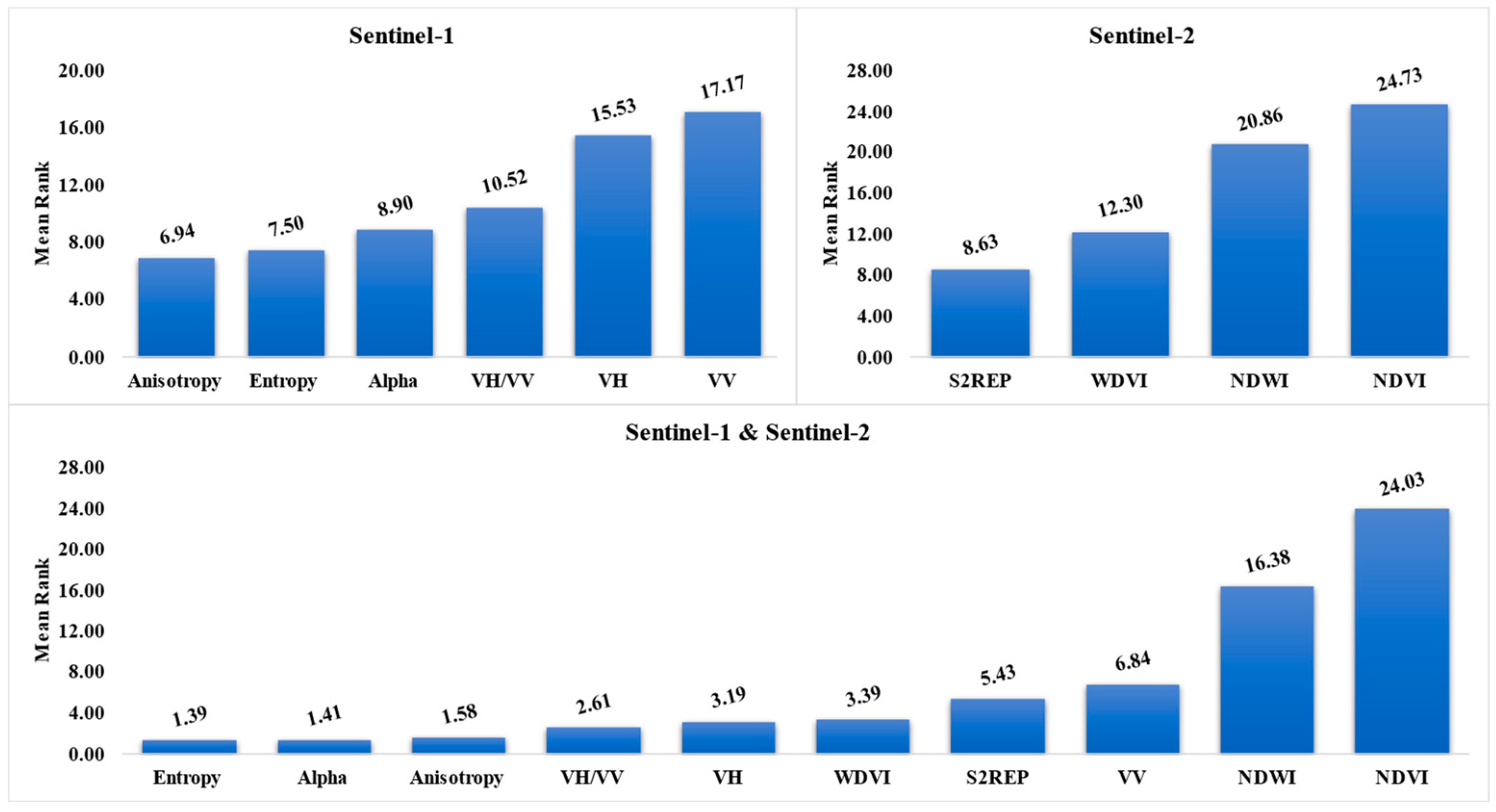
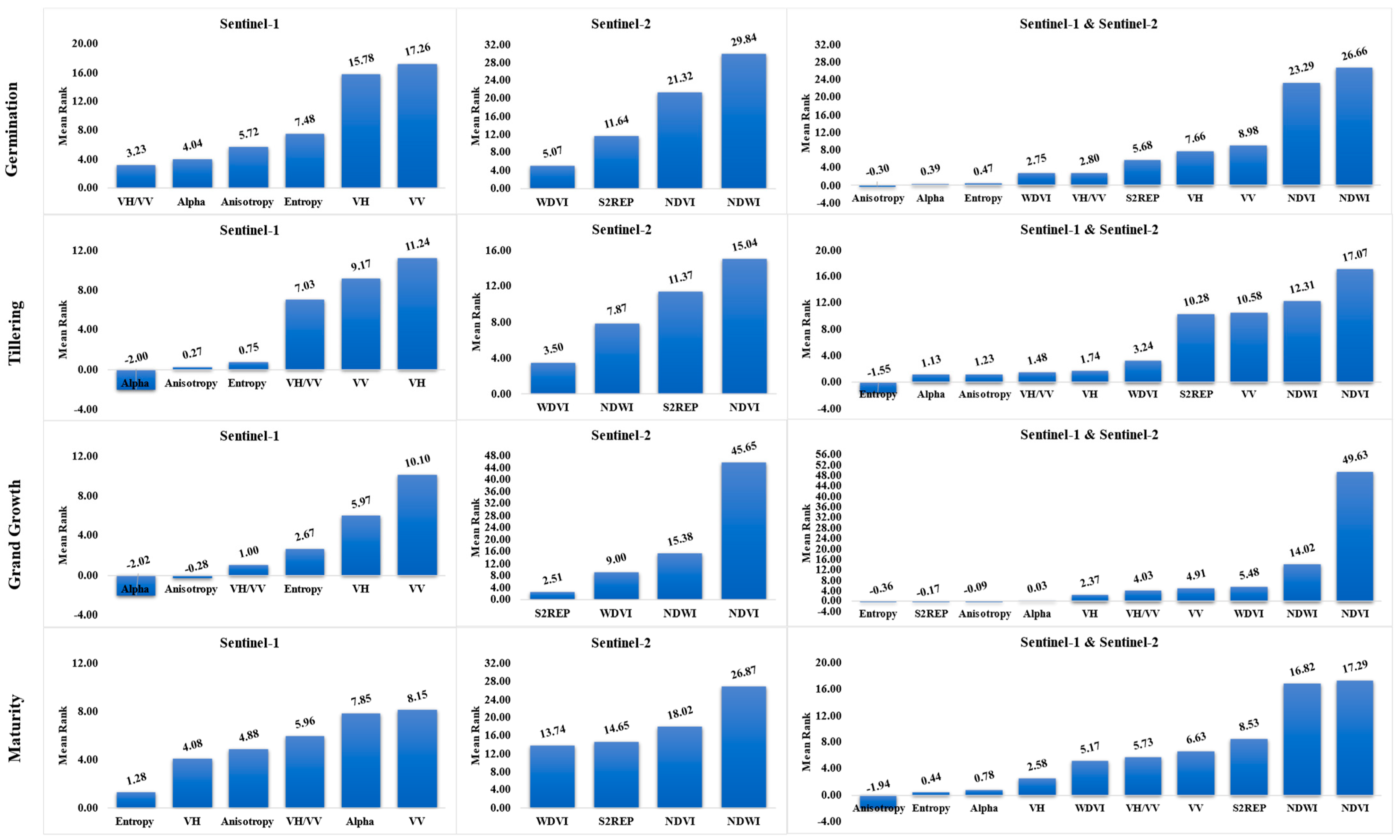
3.2. Variable Importance
4. Discussion
4.1. Sentinel-1 Based Parameters
4.2. Sentinel-2 Based Indices
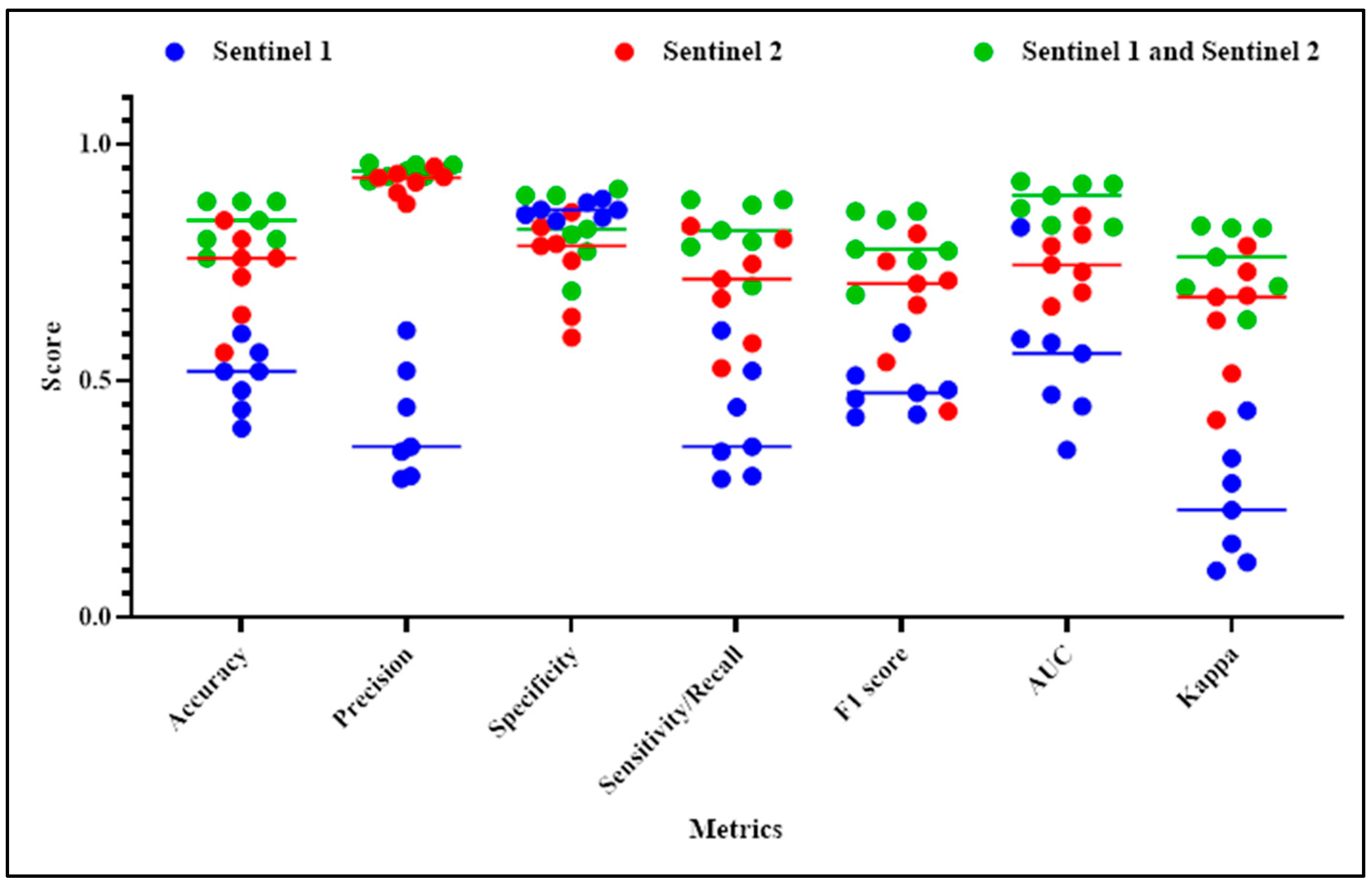
4.3. Combined Sentinel-1 and Sentinel-2 Features
5. Conclusions
Supplementary Materials
Author Contributions
Funding
Data Availability Statement
Acknowledgments
Conflicts of Interest
Abbreviations
| ANN | Artificial Neural Network |
| AUC | Area Under the ROC Curve |
| EVI | Enhanced Vegetation Index |
| FRBS | Fuzzy Rule Based Systems |
| GRD | Ground Range Detected |
| MODIS | Moderate Resolution Imaging Spectroradiometer |
| MSI | Multi-Spectral Instrument |
| NDVI | Normalized Difference Vegetation Index |
| NDWI | Weighted Difference Vegetation Index |
| RF | Random Forest |
| ROC | Receiver Operating Characteristic |
| RVI | Radar Vegetation Index |
| S2REP | Sentinel-2 Red-Edge Position Index |
| SAR | Synthetic Aperture Radar |
| SLC | Single Look Complex |
| SRTM | Shuttle Radar Topography Mission |
| SVM | Support Vector Machine |
| SWIR | Short-Wave Infrared |
| VIRF | Visible Infrared Imaging Radiometer Suite |
| WDRVI | Wide Dynamic Range Vegetation Index |
References
- FAOSTAT. Available online: https://www.fao.org/faostat/en/#home (accessed on 26 May 2022).
- Solomon, S. Sugarcane Agriculture and Sugar Industry in India: At a Glance. Sugar Tech 2014, 16, 113–124. [Google Scholar] [CrossRef]
- Jyothi, K.C. Impact of Policy of Government on Import and Export of Sugar from India. IOSR J. Econ. Financ. 2014, 3, 40–42. [Google Scholar]
- Lieth, H. Phenology and Seasonality Modeling; Springer Science & Business Media: Berlin, Germany, 2013; Volume 8, ISBN 364251863X. [Google Scholar]
- Auffhammer, M.; Ramanathan, V.; Vincent, J.R. Climate Change, the Monsoon, and Rice Yield in India. Clim. Chang. 2012, 111, 411–424. [Google Scholar] [CrossRef]
- Harvey, C.A.; Rakotobe, Z.L.; Rao, N.S.; Dave, R.; Razafimahatratra, H.; Rabarijohn, R.H.; Rajaofara, H.; MacKinnon, J.L. Extreme Vulnerability of Smallholder Farmers to Agricultural Risks and Climate Change in Madagascar. Philos. Trans. R. Soc. B Biol. Sci. 2014, 369, 20130089. [Google Scholar] [CrossRef] [PubMed] [Green Version]
- Samui, R.P.; John, G.; Kulkarni, M.B. Impact of Weather on Yield of Sugarcane at Different Growth Stages. J. Agric. Phys. 2003, 3, 119–125. [Google Scholar]
- Mall, R.K.; Sonkar, G.; Bhatt, D.; Sharma, N.K.; Baxla, A.K.; Singh, K.K. Managing Impact of Extreme Weather Events in Sugarcane in Different Agro-Climatic Zones of Uttar Pradesh. Mausam 2016, 67, 233–250. [Google Scholar] [CrossRef]
- Diao, C. Remote Sensing Phenological Monitoring Framework to Characterize Corn and Soybean Physiological Growing Stages. Remote Sens. Environ. 2020, 248, 111960. [Google Scholar] [CrossRef]
- Palaniswami, C.; Gopalasundaram, P.; Bhaskaran, A. Application of GPS and GIS in Sugarcane Agriculture. Sugar Tech 2011, 13, 360–365. [Google Scholar] [CrossRef]
- Shihua, L.; Jingtao, X.; Ping, N.; Jing, Z.; Hongshu, W.; Jingxian, W. Monitoring Paddy Rice Phenology Using Time Series MODIS Data over Jiangxi Province, China. Int. J. Agric. Biol. Eng. 2014, 7, 28–36. [Google Scholar]
- Wei, W.; Wu, W.; Li, Z.; Yang, P.; Zhou, Q. Selecting the Optimal NDVI Time-Series Reconstruction Technique for Crop Phenology Detection. Intell. Autom. Soft Comput. 2016, 22, 237–247. [Google Scholar] [CrossRef]
- Liu, C.; Shang, J.; Vachon, P.W.; McNairn, H. Multiyear Crop Monitoring Using Polarimetric RADARSAT-2 Data. IEEE Trans. Geosci. Remote Sens. 2012, 51, 2227–2240. [Google Scholar] [CrossRef]
- Ghaderpour, E.; Vujadinovic, T. The Potential of the Least-Squares Spectral and Cross-Wavelet Analyses for Near-Real-Time Disturbance Detection within Unequally Spaced Satellite Image Time Series. Remote Sens. 2020, 12, 2446. [Google Scholar] [CrossRef]
- Ghaderpour, E. JUST: MATLAB and Python Software for Change Detection and Time Series Analysis. GPS Solut. 2021, 25, 85. [Google Scholar] [CrossRef]
- Magdalena, L. Fuzzy Rule-Based Systems. In Springer Handbook of Computational Intelligence; Springer: Berlin/Heidelberg, Germany, 2015; pp. 203–218. [Google Scholar] [CrossRef]
- Sakamoto, T. Refined Shape Model Fitting Methods for Detecting Various Types of Phenological Information on Major US Crops. ISPRS J. Photogramm. Remote Sens. 2018, 138, 176–192. [Google Scholar] [CrossRef]
- Sakamoto, T.; Wardlow, B.D.; Gitelson, A.A.; Verma, S.B.; Suyker, A.E.; Arkebauer, T.J. A Two-Step Filtering Approach for Detecting Maize and Soybean Phenology with Time-Series MODIS Data. Remote Sens. Environ. 2010, 114, 2146–2159. [Google Scholar] [CrossRef]
- Stendardi, L.; Karlsen, S.R.; Niedrist, G.; Gerdol, R.; Zebisch, M.; Rossi, M.; Notarnicola, C. Exploiting Time Series of Sentinel-1 and Sentinel-2 Imagery to Detect Meadow Phenology in Mountain Regions. Remote Sens. 2019, 11, 542. [Google Scholar] [CrossRef] [Green Version]
- Song, Y.; Wang, J. Mapping Winter Wheat Planting Area and Monitoring Its Phenology Using Sentinel-1 Backscatter Time Series. Remote Sens. 2019, 11, 449. [Google Scholar] [CrossRef] [Green Version]
- Mercier, A.; Betbeder, J.; Baudry, J.; Denize, J.; Leroux, V.; Roger, J.-L.; Spicher, F.; Hubert-Moy, L. Evaluation of Sentinel-1 and-2 Time Series to Derive Crop Phenology and Biomass of Wheat and Rapeseed: Northern France and Brittany Case Studies. In Proceedings of the Remote Sensing for Agriculture, Ecosystems, and Hydrology XXI, Strasbourg, France, 9–11 September 2019; Volume 11149, p. 1114903. [Google Scholar]
- Gaetano, R.; Cozzolino, D.; D’Amiano, L.; Verdoliva, L.; Poggi, G. Fusion of SAR-Optical Data for Land Cover Monitoring. In Proceedings of the 2017 IEEE International Geoscience and Remote Sensing Symposium (IGARSS), Fort Worth, TX, USA, 23–28 July 2017; IEEE: Piscataway, NJ, USA, 2017; pp. 5470–5473. [Google Scholar]
- Li, X.; Du, Z.; Huang, Y.; Tan, Z. A Deep Translation (GAN) Based Change Detection Network for Optical and SAR Remote Sensing Images. ISPRS J. Photogramm. Remote Sens. 2021, 179, 14–34. [Google Scholar] [CrossRef]
- Song, X.-P.; Huang, W.; Hansen, M.C.; Potapov, P. An Evaluation of Landsat, Sentinel-2, Sentinel-1 and MODIS Data for Crop Type Mapping. Sci. Remote Sens. 2021, 3, 100018. [Google Scholar] [CrossRef]
- Haldar, D.; Verma, A.; Kumar, S.; Chauhan, P. Estimation of Mustard and Wheat Phenology Using Multi-Date Shannon Entropy and Radar Vegetation Index from Polarimetric Sentinel-1. Geocarto Int. 2021, 1–28. [Google Scholar] [CrossRef]
- Chen, C.F.; Son, N.T.; Chen, C.R.; Chang, L.Y.; Chiang, S.H. Rice Crop Mapping Using Sentinel-1A Phenological Metrics. Int. Arch. Photogramm. Remote Sens. Spat. Inf. Sci. 2016, 41. [Google Scholar] [CrossRef]
- Narin, O.G.; Abdikan, S. Monitoring of Phenological Stage and Yield Estimation of Sunflower Plant Using Sentinel-2 Satellite Images. Geocarto Int. 2020, 37, 1–15. [Google Scholar] [CrossRef]
- Haldar, D.; Tripathy, R.; Dave, V.; Dave, R.; Bhattacharya, B.K.; Misra, A. Monitoring Cotton Crop Condition through Synergy of Optical and Radar Remote Sensing. Geocarto Int. 2022, 37, 377–395. [Google Scholar] [CrossRef]
- Singh, D.; Singh, S.; Shekhar, C.; Singh, R.; Rao, V.U.M. Agroclimatic Features of Hisar Region; AICRP on Agrometeorology, Department of Agril Meteorology, College of of Agriculture, CCS Haryana Agricultural University: Haryana, India, 2010. [Google Scholar]
- Ahlawat, I.; Sheoran, H.S.; Dahiya, G.; Sihag, P. Analysis of Sentinel-1 Data for Regional Crop Classification: A Multi-Data Approach for Rabi Crops of District Hisar (Haryana). J. Appl. Nat. Sci. 2020, 12, 165–170. [Google Scholar] [CrossRef]
- Lee, J.-S.; Grunes, M.R.; de Grandi, G. Polarimetric SAR Speckle Filtering and Its Implication for Classification. IEEE Trans. Geosci. Remote Sens. 1999, 37, 2363–2373. [Google Scholar]
- Farr, T.G.; Rosen, P.A.; Caro, E.; Crippen, R.; Duren, R.; Hensley, S.; Kobrick, M.; Paller, M.; Rodriguez, E.; Roth, L. The Shuttle Radar Topography Mission. Rev. Geophys. 2007, 45, 1–33. [Google Scholar] [CrossRef] [Green Version]
- Denize, J.; Hubert-Moy, L.; Betbeder, J.; Corgne, S.; Baudry, J.; Pottier, E. Evaluation of Using Sentinel-1 and-2 Time-Series to Identify Winter Land Use in Agricultural Landscapes. Remote Sens. 2018, 11, 37. [Google Scholar] [CrossRef] [Green Version]
- Gascon, F.; Bouzinac, C.; Thépaut, O.; Jung, M.; Francesconi, B.; Louis, J.; Lonjou, V.; Lafrance, B.; Massera, S.; Gaudel-Vacaresse, A. Copernicus Sentinel-2A Calibration and Products Validation Status. Remote Sens. 2017, 9, 584. [Google Scholar] [CrossRef] [Green Version]
- Gamon, J.A.; Field, C.B.; Goulden, M.L.; Griffin, K.L.; Hartley, A.E.; Joel, G.; Penuelas, J.; Valentini, R. Relationships between NDVI, Canopy Structure, and Photosynthesis in Three Californian Vegetation Types. Ecol. Appl. 1995, 5, 28–41. [Google Scholar] [CrossRef] [Green Version]
- Grace, J.; Nichol, C.; Disney, M.; Lewis, P.; Quaife, T.; Bowyer, P. Can We Measure Terrestrial Photosynthesis from Space Directly, Using Spectral Reflectance and Fluorescence? Glob. Change Biol. 2007, 13, 1484–1497. [Google Scholar] [CrossRef]
- Karnieli, A.; Agam, N.; Pinker, R.T.; Anderson, M.; Imhoff, M.L.; Gutman, G.G.; Panov, N.; Goldberg, A. Use of NDVI and Land Surface Temperature for Drought Assessment: Merits and Limitations. J. Clim. 2010, 23, 618–633. [Google Scholar] [CrossRef]
- Gao, B.-C. NDWI—A Normalized Difference Water Index for Remote Sensing of Vegetation Liquid Water from Space. Remote Sens. Environ. 1996, 58, 257–266. [Google Scholar] [CrossRef]
- Jackson, T.J.; Chen, D.; Cosh, M.; Li, F.; Anderson, M.; Walthall, C.; Doriaswamy, P.; Hunt, E.R. Vegetation Water Content Mapping Using Landsat Data Derived Normalized Difference Water Index for Corn and Soybeans. Remote Sens. Environ. 2004, 92, 475–482. [Google Scholar] [CrossRef]
- Serrano, J.; Shahidian, S.; Marques da Silva, J. Evaluation of Normalized Difference Water Index as a Tool for Monitoring Pasture Seasonal and Inter-Annual Variability in a Mediterranean Agro-Silvo-Pastoral System. Water 2019, 11, 62. [Google Scholar] [CrossRef] [Green Version]
- Bouman, B.A.M.; van Kasteren, H.W.J.; Uenk, D. Standard Relations to Estimate Ground Cover and LAI of Agricultural Crops from Reflectance Measurements. Eur. J. Agron. 1992, 1, 249–262. [Google Scholar] [CrossRef]
- Guyot, G.; Baret, F. Utilisation de La Haute Resolution Spectrale Pour Suivre l’etat Des Couverts Vegetaux. In Proceedings of the Spectral Signatures of Objects in Remote Sensing, Aussois, France, 18–22 January 1988; Volume 287, p. 279. [Google Scholar]
- Clevers, J.; de Jong, S.M.; Epema, G.F.; Addink, E.A.; van der Meer, F.; Skidmore, A.K. Meris and the Red-Edge Index. In Proceedings of the Second EARSeL Workshop on Imaging Spectroscopy, Enschede, The Netherlands, 11–13 July 2000. [Google Scholar]
- Rouse, B.T.; Wells, R.J.H.; Warner, N.L. Proportion of T and B Lymphocytes in Lesions of Marek’s Disease: Theoretical Implications for Pathogenesis. J. Immunol. 1973, 110, 534–539. [Google Scholar]
- Gao, B.C.; Goetzt, A.F. Retrieval of equivalent water thickness and information related to biochemical components of vegetation canopies from AVIRIS data. Remote Sens. Environ. 1995, 52, 155–162. [Google Scholar] [CrossRef]
- Clevers, J. The Derivation of a Simplified Reflectance Model for the Estimation of Leaf Area Index. Remote Sens. Environ. 1988, 25, 53–69. [Google Scholar] [CrossRef]
- Maxwell, A.E.; Warner, T.A.; Guillén, L.A. Accuracy Assessment in Convolutional Neural Network-Based Deep Learning Remote Sensing Studies—Part 1: Literature Review. Remote Sens. 2021, 13, 2450. [Google Scholar] [CrossRef]
- Sarlis, N.V.; Skordas, E.S.; Christopoulos, S.-R.G.; Varotsos, P.A. Natural Time Analysis: The Area under the Receiver Operating Characteristic Curve of the Order Parameter Fluctuations Minima Preceding Major Earthquakes. Entropy 2020, 22, 583. [Google Scholar] [CrossRef]
- Cox, D.R. The Regression Analysis of Binary Sequences. J. R. Stat. Soc. Ser. B Methodol. 1958, 20, 215–232. [Google Scholar] [CrossRef]
- Walker, S.H.; Duncan, D.B. Estimation of the Probability of an Event as a Function of Several Independent Variables. Biometrika 1967, 54, 167–179. [Google Scholar] [CrossRef] [PubMed]
- Tabachnick, B.G.; Fidell, L.S.; Ullman, J.B. Using Multivariate Statistics; Pearson: Boston, MA, USA, 2007; Volume 5. [Google Scholar]
- Good, I.J. Probability and the Weighing of Evidence. Biometrika 1951, 38, 485. [Google Scholar]
- Vapnik, V. The Nature of Statistical Learning Theory; Springer Science & Business Media: Berlin, Germany, 1999; ISBN 0387987800. [Google Scholar]
- Nizar, A.H.; Dong, Z.Y.; Wang, Y. Power Utility Nontechnical Loss Analysis with Extreme Learning Machine Method. IEEE Trans. Power Syst. 2008, 23, 946–955. [Google Scholar] [CrossRef]
- Berwick, R. An Idiot’s Guide to Support Vector Machines (SVMs). Retrieved Oct. 2003, 21, 2011. [Google Scholar]
- Hastie, T.; Tibshirani, R.; Friedman, J. High-Dimensional Problems: P n. In The Elements of Statistical Learning; Springer: Berlin/Heidelberg, Germany, 2009; pp. 649–698. [Google Scholar]
- Murthy, S.K. Automatic Construction of Decision Trees from Data: A Multi-Disciplinary Survey. Data Min. Knowl. Discov. 1998, 2, 345–389. [Google Scholar] [CrossRef]
- Kotsiantis, S.B.; Zaharakis, I.; Pintelas, P. Supervised Machine Learning: A Review of Classification Techniques. Emerg. Artif. Intell. Appl. Comput. Eng. 2007, 160, 3–24. [Google Scholar]
- Hunt, E.B.; Marin, J.; Stone, P. Experiments in Induction; Academic Press: New York, NY, USA, 1966. [Google Scholar]
- Breiman, L.; Ihaka, R. Nonlinear Discriminant Analysis via Scaling and ACE; Department of Statistics, University of California: Los Angeles, CA, USA, 1984. [Google Scholar]
- Liaw, A.; Wiener, M. Classification and Regression by RandomForest. R News 2002, 2, 18–22. [Google Scholar]
- Probst, P.; Wright, M.N.; Boulesteix, A. Hyperparameters and Tuning Strategies for Random Forest. Wiley Interdiscip. Rev. Data Min. Knowl. Discov. 2019, 9, e1301. [Google Scholar] [CrossRef] [Green Version]
- Gupta, T.K.; Raza, K. Optimization of ANN Architecture: A Review on Nature-Inspired Techniques. In Machine Learning in Bio-Signal Analysis and Diagnostic Imaging; Academic Press: Cambridge, MA, USA, 2019; pp. 159–182. [Google Scholar]
- Neocleous, C.; Schizas, C. Artificial Neural Network Learning: A Comparative Review. In Proceedings of the Hellenic Conference on Artificial Intelligence, Thessaloniki, Greece, 11–12 April 2002; Springer: Berlin/Heidelberg, Germany, 2002; pp. 300–313. [Google Scholar]
- Rumelhart, D.E.; Hinton, G.E.; Williams, R.J. Learning Representations by Back-Propagating Errors. Nature 1986, 323, 533–536. [Google Scholar] [CrossRef]
- Zadeh, L.A.; Klir, G.J.; Yuan, B. Fuzzy Sets, Fuzzy Logic, and Fuzzy Systems: Selected Papers; World Scientific: Singapore, 1996; Volume 6, ISBN 9810224214. [Google Scholar]
- Sugeno, M.; Yasukawa, T. A Fuzzy-Logic-Based Approach to Qualitative Modeling. IEEE Trans. Fuzzy Syst. 1993, 1, 7–31. [Google Scholar] [CrossRef] [Green Version]
- Pedrycz, W. Fuzzy Modelling: Paradigms and Practice; Springer Science & Business Media: Berlin, Germany, 1996; ISBN 0792397037. [Google Scholar]
- Ishibuchi, H.; Nakashima, T. Effect of Rule Weights in Fuzzy Rule-Based Classification Systems. IEEE Trans. Fuzzy Syst. 2001, 9, 506–515. [Google Scholar] [CrossRef]
- Lopez-Sanchez, J.M.; Vicente-Guijalba, F.; Ballester-Berman, J.D.; Cloude, S.R. Polarimetric Response of Rice Fields at C-Band: Analysis and Phenology Retrieval. IEEE Trans. Geosci. Remote Sens. 2013, 52, 2977–2993. [Google Scholar] [CrossRef] [Green Version]
- Dey, S.; Bhogapurapu, N.; Bhattacharya, A.; Mandal, D.; Lopez-Sanchez, J.M.; McNairn, H.; Frery, A.C. Rice Phenology Mapping Using Novel Target Characterization Parameters from Polarimetric SAR Data. Int. J. Remote Sens. 2021, 42, 5515–5539. [Google Scholar] [CrossRef]
- Varghese, A.O.; Joshi, A.K. Polarimetric Classification of C-Band SAR Data for Forest Density Characterization. Curr. Sci. 2015, 108, 100–106. [Google Scholar]
- Mandal, D.; Kumar, V.; Ratha, D.; Dey, S.; Bhattacharya, A.; Lopez-Sanchez, J.M.; McNairn, H.; Rao, Y.S. Dual Polarimetric Radar Vegetation Index for Crop Growth Monitoring Using Sentinel-1 SAR Data. Remote Sens. Environ. 2020, 247, 111954. [Google Scholar] [CrossRef]
- Harfenmeister, K.; Spengler, D.; Weltzien, C. Analyzing Temporal and Spatial Characteristics of Crop Parameters Using Sentinel-1 Backscatter Data. Remote Sens. 2019, 11, 1569. [Google Scholar] [CrossRef] [Green Version]
- Fieuzal, R.; Baup, F.; Marais-Sicre, C. Monitoring Wheat and Rapeseed by Using Synchronous Optical and Radar Satellite Data—From Temporal Signatures to Crop Parameters Estimation. Adv. Remote Sens. 2013, 2, 33222. [Google Scholar] [CrossRef] [Green Version]
- Cookmartin, G.; Saich, P.; Quegan, S.; Cordey, R.; Burgess-Allen, P.; Sowter, A. Modeling Microwave Interactions with Crops and Comparison with ERS-2 SAR Observations. IEEE Trans. Geosci. Remote Sens. 2000, 38, 658–670. [Google Scholar] [CrossRef]
- Khabbazan, S.; Vermunt, P.; Steele-Dunne, S.; Ratering Arntz, L.; Marinetti, C.; van der Valk, D.; Iannini, L.; Molijn, R.; Westerdijk, K.; van der Sande, C. Crop Monitoring Using Sentinel-1 Data: A Case Study from The Netherlands. Remote Sens. 2019, 11, 1887. [Google Scholar] [CrossRef] [Green Version]
- Wiseman, G.; McNairn, H.; Homayouni, S.; Shang, J. RADARSAT-2 Polarimetric SAR Response to Crop Biomass for Agricultural Production Monitoring. IEEE J. Sel. Top. Appl. Earth Obs. Remote Sens. 2014, 7, 4461–4471. [Google Scholar] [CrossRef]
- Moran, M.S.; Alonso, L.; Moreno, J.F.; Mateo, M.P.C.; de La Cruz, D.F.; Montoro, A. A RADARSAT-2 Quad-Polarized Time Series for Monitoring Crop and Soil Conditions in Barrax, Spain. IEEE Trans. Geosci. Remote Sens. 2011, 50, 1057–1070. [Google Scholar] [CrossRef]
- Ryu, J.-H.; Jeong, H.; Cho, J. Performances of Vegetation Indices on Paddy Rice at Elevated Air Temperature, Heat Stress, and Herbicide Damage. Remote Sens. 2020, 12, 2654. [Google Scholar] [CrossRef]
- Gnyp, M.L.; Miao, Y.; Yuan, F.; Ustin, S.L.; Yu, K.; Yao, Y.; Huang, S.; Bareth, G. Hyperspectral Canopy Sensing of Paddy Rice Aboveground Biomass at Different Growth Stages. Field Crops Res. 2014, 155, 42–55. [Google Scholar] [CrossRef]
- Mourad, R.; Jaafar, H.; Anderson, M.; Gao, F. Assessment of Leaf Area Index Models Using Harmonized Landsat and Sentinel-2 Surface Reflectance Data over a Semi-Arid Irrigated Landscape. Remote Sens. 2020, 12, 3121. [Google Scholar] [CrossRef]
- Huang, J. Vegetation Properties Relationships from Spectral Bands and Vegetation Indices from Operational Satellites; The University of Manchester: Manchester, UK, 2006; ISBN 1392123283. [Google Scholar]
- Kotsianti, S.B.; Kanellopoulos, D. Combining Bagging, Boosting and Dagging for Classification Problems. In Proceedings of the International Conference on Knowledge-Based and Intelligent Information and Engineering Systems, Vietri sul Mare, Italy, September 12-14, 2007; Springer: Berlin, Germany, 2007; pp. 493–500. [Google Scholar]
- Verikas, A.; Gelzinis, A.; Bacauskiene, M. Mining Data with Random Forests: A Survey and Results of New Tests. Pattern Recognit. 2011, 44, 330–349. [Google Scholar] [CrossRef]
- Veloso, A.; Mermoz, S.; Bouvet, A.; le Toan, T.; Planells, M.; Dejoux, J.-F.; Ceschia, E. Understanding the Temporal Behavior of Crops Using Sentinel-1 and Sentinel-2-like Data for Agricultural Applications. Remote Sens Environ. 2017, 199, 415–426. [Google Scholar] [CrossRef]
- Tian, H.; Wu, M.; Wang, L.; Niu, Z. Mapping Early, Middle and Late Rice Extent Using Sentinel-1A and Landsat-8 Data in the Poyang Lake Plain, China. Sensors 2018, 18, 185. [Google Scholar] [CrossRef] [Green Version]
- Gašparović, M.; Dobrinić, D. Comparative Assessment of Machine Learning Methods for Urban Vegetation Mapping Using Multitemporal Sentinel-1 Imagery. Remote Sens. 2020, 12, 1952. [Google Scholar] [CrossRef]
- Hu, Y.; Zeng, H.; Tian, F.; Zhang, M.; Wu, B.; Gilliams, S.; Li, S.; Li, Y.; Lu, Y.; Yang, H. An Interannual Transfer Learning Approach for Crop Classification in the Hetao Irrigation District, China. Remote Sens. 2022, 14, 1208. [Google Scholar] [CrossRef]
- Feyisa, G.L.; Palao, L.K.; Nelson, A.; Gumma, M.K.; Paliwal, A.; Win, K.T.; Nge, K.H.; Johnson, D.E. Characterizing and Mapping Cropping Patterns in a Complex Agro-Ecosystem: An Iterative Participatory Mapping Procedure Using Machine Learning Algorithms and MODIS Vegetation Indices. Comput. Electron. Agric. 2020, 175, 105595. [Google Scholar] [CrossRef]


| Index | Formula | Sentinel-2 | Range | References |
|---|---|---|---|---|
| NDVI | −1 to 1 | [44] | ||
| NDWI | −1 to 1 | [38,45] | ||
| WDVI | −1 to 1 | [46] | ||
| S2REP | ) | ) | 650 to 750 | [42] |
| Accuracy | Precision | Specificity | Sensitivity/ Recall | F1 Score | AUC | Kappa | |
|---|---|---|---|---|---|---|---|
| Sentinel-1 | |||||||
| Decision tree | 40.00% | 29.30% | 83.83% | 40.83% | 0.42 | 0.56 | 0.10 |
| FRBS | 56.00% | 44.45% | 87.77% | 67.32% | 0.48 | 0.59 | 0.28 |
| Logistic | 44.00% | 35.04% | 84.50% | 33.33% | 0.43 | 0.45 | 0.12 |
| Naïve Bayes | 52.00% | 52.14% | 86.25% | 50.89% | 0.48 | 0.58 | 0.34 |
| Neural net | 48.00% | 29.87% | 85.11% | 23.89% | 0.51 | 0.35 | 0.16 |
| Random forest | 60.00% | 60.66% | 88.50% | 67.98% | 0.60 | 0.83 | 0.44 |
| SVM | 52.00% | 36.12% | 86.19% | 38.89% | 0.46 | 0.47 | 0.23 |
| Sentinel-2 | |||||||
| Decision tree | 80.00% | 93.78% | 82.59% | 80.06% | 0.75 | 0.85 | 0.73 |
| FRBS | 64.00% | 89.81% | 63.57% | 57.98% | 0.54 | 0.69 | 0.52 |
| Logistic | 76.00% | 92.99% | 78.57% | 71.53% | 0.71 | 0.79 | 0.68 |
| Naïve Bayes | 56.00% | 87.51% | 59.20% | 52.67% | 0.44 | 0.66 | 0.42 |
| Neural net | 84.00% | 95.35% | 85.71% | 82.76% | 0.81 | 0.81 | 0.79 |
| Random forest | 72.00% | 92.01% | 75.45% | 67.42% | 0.66 | 0.73 | 0.63 |
| SVM | 76.00% | 93.13% | 79.02% | 74.73% | 0.71 | 0.75 | 0.68 |
| Sentinel-1 and Sentinel-2 | |||||||
| Decision tree | 76.00% | 92.28% | 69.05% | 70.09% | 0.68 | 0.83 | 0.63 |
| FRBS | 80.00% | 93.31% | 82.14% | 79.49% | 0.78 | 0.89 | 0.70 |
| Logistic | 80.00% | 94.42% | 80.95% | 81.81% | 0.78 | 0.83 | 0.76 |
| Naïve Bayes | 84.00% | 96.11% | 90.58% | 87.21% | 0.84 | 0.92 | 0.83 |
| Neural net | 88.00% | 93.31% | 77.38% | 78.38% | 0.75 | 0.87 | 0.70 |
| Random forest | 88.00% | 95.74% | 89.29% | 88.32% | 0.86 | 0.92 | 0.82 |
| SVM | 88.00% | 95.74% | 89.29% | 88.32% | 0.86 | 0.92 | 0.82 |
| Models | Sentinel-1 | Sentinel-2 | Sentinel-1 and Sentinel-2 | |||
|---|---|---|---|---|---|---|
| Accuracy | Kappa | Accuracy | Kappa | Accuracy | Kappa | |
| Decision tree | f, c | f, c | b, a | b, a | d, d | d, b |
| FRBS | b, c | d, c | e, b | e, b | c, a | c, a |
| Logistic | e, c | e, c | c, b | c, b | c, a | b, a |
| Naïve Bayes | c, c | b, c | f, b | f, b | b, a | a, a |
| Neural net | d, c | e, c | a, b | a, b | a, a | c, a |
| Random forest | a, c | a, c | d, b | d, b | a, a | a, a |
| SVM | c, c | c, c | c, b | c, b | a, a | a, a |
Publisher’s Note: MDPI stays neutral with regard to jurisdictional claims in published maps and institutional affiliations. |
© 2022 by the authors. Licensee MDPI, Basel, Switzerland. This article is an open access article distributed under the terms and conditions of the Creative Commons Attribution (CC BY) license (https://creativecommons.org/licenses/by/4.0/).
Share and Cite
Yeasin, M.; Haldar, D.; Kumar, S.; Paul, R.K.; Ghosh, S. Machine Learning Techniques for Phenology Assessment of Sugarcane Using Conjunctive SAR and Optical Data. Remote Sens. 2022, 14, 3249. https://doi.org/10.3390/rs14143249
Yeasin M, Haldar D, Kumar S, Paul RK, Ghosh S. Machine Learning Techniques for Phenology Assessment of Sugarcane Using Conjunctive SAR and Optical Data. Remote Sensing. 2022; 14(14):3249. https://doi.org/10.3390/rs14143249
Chicago/Turabian StyleYeasin, Md, Dipanwita Haldar, Suresh Kumar, Ranjit Kumar Paul, and Sonaka Ghosh. 2022. "Machine Learning Techniques for Phenology Assessment of Sugarcane Using Conjunctive SAR and Optical Data" Remote Sensing 14, no. 14: 3249. https://doi.org/10.3390/rs14143249