Assessing Climate Influence on Spatiotemporal Dynamics of Macrophytes in Eutrophicated Reservoirs by Remotely Sensed Time Series

Abstract

The overgrowth of macrophytes is a recurrent problem within reservoirs of urbanized and industrialized areas, a condition triggered by the damming of rivers and other human activities. Although the occurrence of aquatic plants in waterbodies has been widely monitored using remote sensing, the influence of climate variables on macrophyte spatiotemporal dynamics is rarely considered in studies developed for medium scales to long periods of time. We hypothesize that the spatial dispersion of macrophytes has its natural rhythms influenced by climate fluctuations, and, as such, its effects on the heterogeneous spatial distribution of this vegetation should be considered in the monitoring of water bodies. A eutrophic reservoir is selected for study, which uses the Normalized Difference Vegetation Index (NDVI) as a proxy for macrophytes. Landsat’s NDVI long-term time series are constructed and matched with the Climate Variable (CV) from the National Oceanic and Atmospheric Administration (NOAA) to assess the spatiotemporal dynamics of aquatic plants and their associated climate triggers. The NDVI and CV time series and their seasonal and trend components are correlated for the entire reservoir, compartments, and segmented areas of the water body. Granger-causality of these climate variables show that they contribute to describe and predict the spatial dispersion of macrophytes.

1. Introduction

The degradation of water resources is a consequence of cultural and natural factors, mainly related to the accelerated occupation of springs and margins of rivers, lakes, and reservoirs. Anthropogenic activities degrade water quality, causing the aquatic environments to increasingly become eutrophicated, favoring aquatic vegetation proliferation, and consequently leading to loss of biodiversity. River damming for electric power production usually triggers strong impacts on aquatic ecosystems, especially in reservoirs located in urbanized and industrialized areas. It is essential, therefore, to monitor the distribution and variations of macrophytes [1], and to understand and quantify the environmental factors that influence their distribution patterns in different aquatic environments [2].

Due to the spatiotemporal scales involved in water resources scenarios, they are scaled for monitoring using remote sensing products, i.e., through the Normalized Difference Vegetation Index (NDVI). NDVI has been widely used to monitor disturbances in water availability and quality [3,4,5,6,7] as it allows for several estimates in space and time (including seasonal behavior) to be performed [8,9,10,11]. In [12], this vegetation index is used to detect both open water and the subsequent vegetation response in Gwyndir wetlands, Australia, and the authors developed a decision tree to identify and map the likely flood extent from an NDVI time series. In [13], it is reported that there was an acceptable correlation between climate data and vegetation indices aggregated at the biome-level in the Eastern Cape of South Africa, even though the biome comprised complex vegetation types.

With respect to monitoring macrophytes’ spatiotemporal distribution caused by both anthropogenic and environmental impacts, ref. [14] found that NDVI allowed for the identification of floating macrophytes’ abnormal growth, while [15] opined that consistent, spatialized details of key phenological features are needed to elucidate the main drivers behind the seasonal dynamicity of aquatic vegetation in order to minimize the potential impacts of macrophyte overabundance. In [16], it is found that NDVI time series are suitable for identifying areas where the vegetation cover had increased or decreased and indicated that decadal trends of annual precipitation coincided with the detected larger NDVI trend areas

For their part, ref. [17] observed temporal correspondence between reservoir storage located in two watersheds and the time series from satellite images with land surface temperature, indicating that the best correlation coincided with areas where significant decreases in precipitation were expected. When studying the influence of climate changes on hydrology in the Brazilian Pantanal, ref. [18] analyzed the temporal relationship between mean summer rainy days and key climate variables provided by NOAA/ESRL, finding the highest linear correlations for precipitable water and air temperature. In regard to the dynamics of aquatic vegetation and their relations with environmental factors, ref. [19] reported that for Lake Taihu in China, inter-annual distribution area variations had significant positive correlations with air temperature, water level, and certain quality parameters. The aforementioned studies showcase the potential of employing remotely sensed products to monitor macrophytes’ behaviors.

Although efforts to monitor water resources are directed at large water bodies due to their spatial coverage that favors the use of remotely sensed data (e.g., [20,21,22]), it should be pointed out that even the smallest highly eutrophic reservoirs exposed to irregular, drastic, and punctual anthropic interventions are subject to impacts that manifest themselves cyclically in the aquatic environment. These cyclical behaviors are influenced by climate changes [23] and, as such, can also be better monitored by incorporating the temporal dimension into the integrated analysis.

In this sense, we hypothesize that the spatial dispersions of floating macrophytes have their natural rhythms influenced by climate fluctuations, and, as such, their effects on the heterogeneous spatial distribution of this vegetation must be considered in water body monitoring. This study proposes to explore long-term time series of Landsat images integrating climate variables in the analysis, since factors such as temperature, precipitation, and wind direction influence the dispersion of macrophyte banks in reservoirs. In order to evaluate our proposition, a study area located in a highly urbanized and industrialized region of the São Paulo state, Brazil, was chosen, which has the recurrent problem of overabundance of macrophytes.

2. Methods

To analyze the influence of climatic variables on the behavior of macrophytes in an aquatic environment, the Salto Grande reservoir was selected as the study area, as it presents a recurrent problem of macrophyte overgrowth. Understanding these relationships leads to the possibility of incorporating the analysis of climate data into the monitoring and management of floating aquatic vegetation.

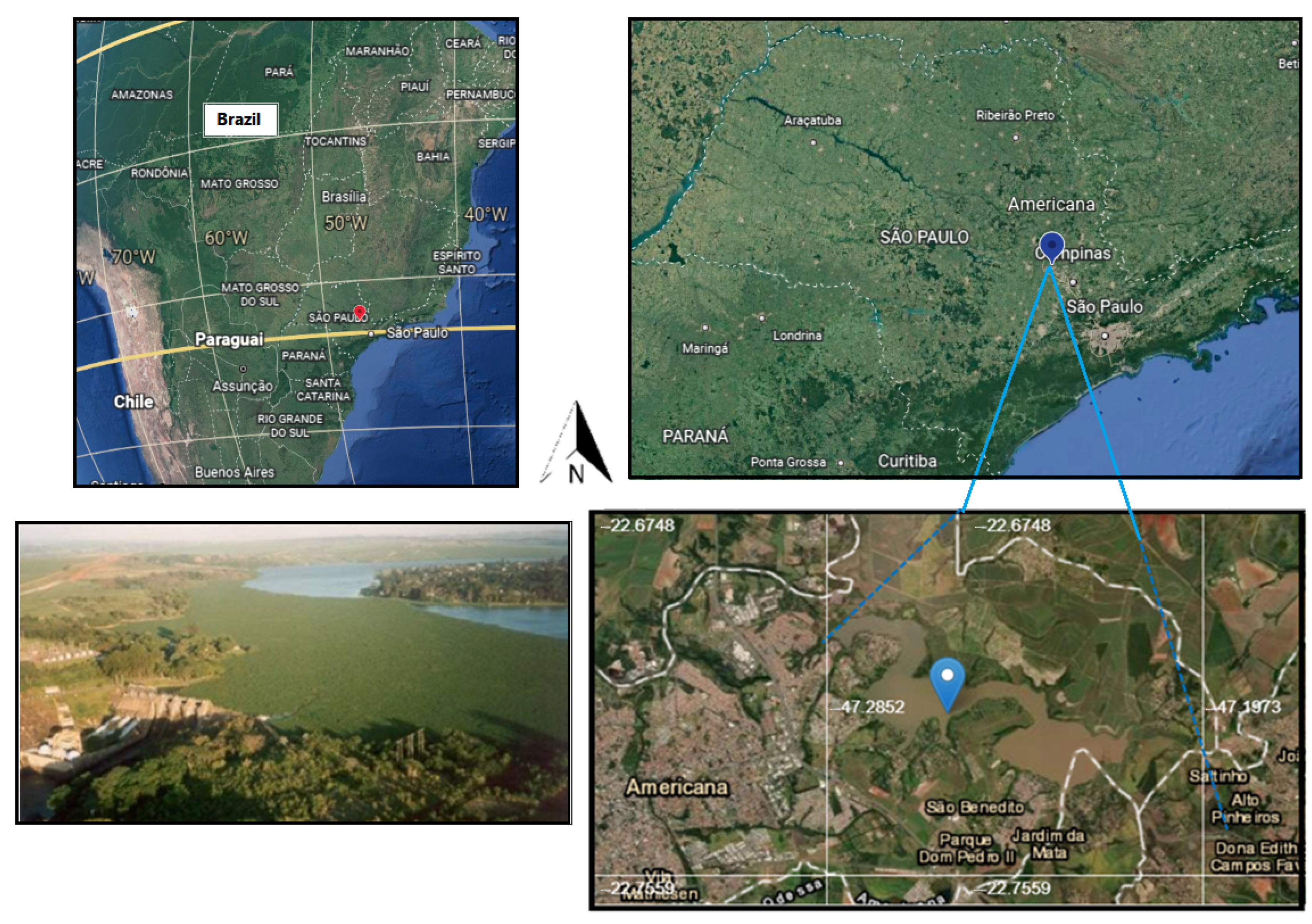
2.1. Salto Grande Reservoir (Brazil)

The Salto Grande reservoir is in the State of São Paulo, Brazil, and is within 3 municipalities: Americana, Paulínia, and Nova Odessa (Figure 1). In this region, the summer is long, hot, and humid, with frequent rains, while the winter is short and mild. Temperature and precipitation vary throughout the year, with the highest temperatures and rainfall occurring from November to May. The seasonal variation in humidity is also extreme; December, January, and February are the wettest months, and June, July, and August the driest. The incident short-wave solar energy has moderate seasonal variations, and the change in wind speed is small throughout the year [24].

The reservoir was formed by the damming of the Atibaia River for the installation of the Americana hydroelectric power plant in 1949. It has a perimeter of about 64 km, and the flooded area varies between approximately 10 km² and 13 km². Human occupation in its surroundings triggers a process of environmental degradation and reduced water quality and has causes overgrowth of macrophytes with critical impacts in the last decade [25].

2.2. Temporal Datasets

The dynamics of the macrophytes’ occurrence in the reservoir was studied from temporal datasets obtained from two sources: data extracted from surface reflectance Landsat images available on demand at the USGS (United States Geological Survey) Earth Explorer website, and data obtained from the National Oceanic and Atmospheric Administration/Earth System Research Laboratory (NOAA/ESRL) website.

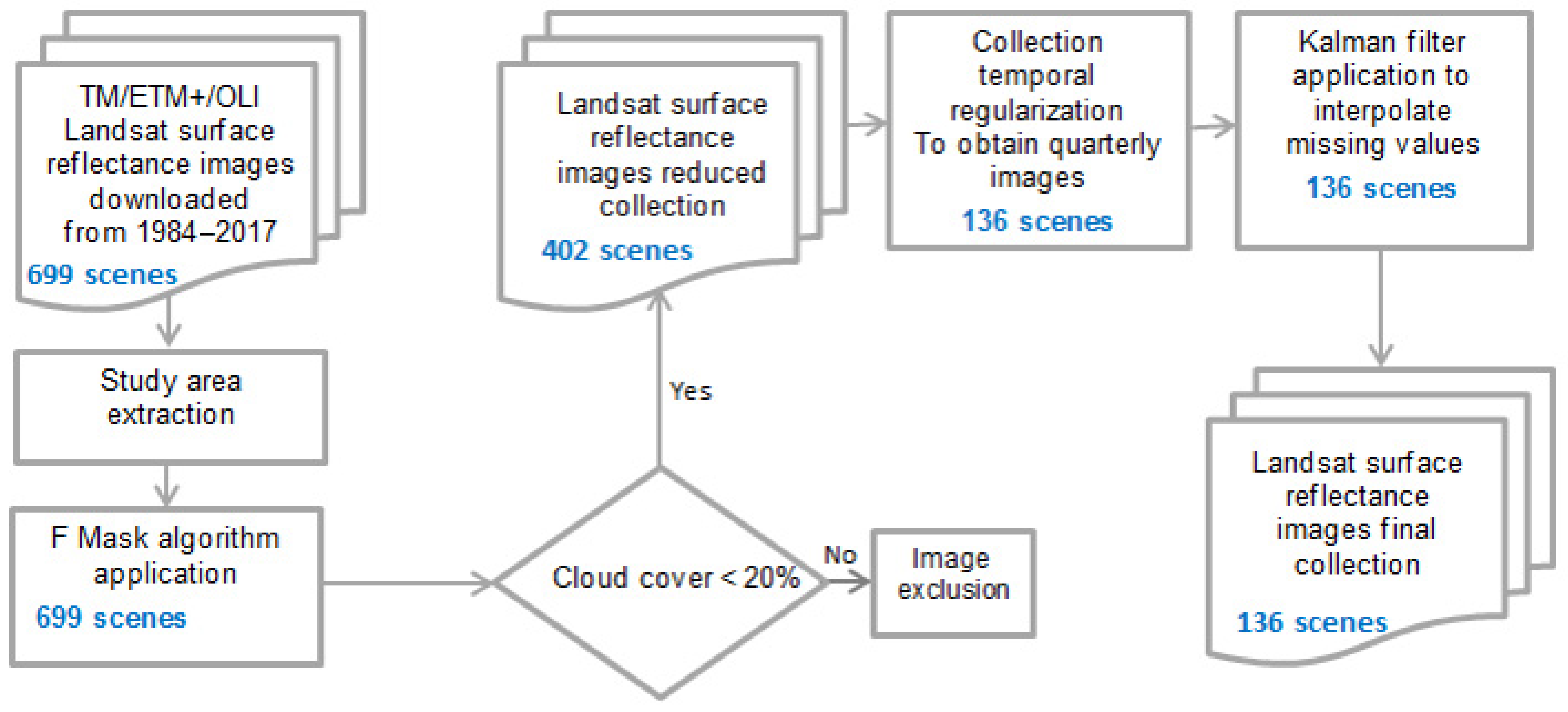
2.2.1. Landsat Image Acquisition

The Landsat multispectral images used to compose the NDVI time series were acquired by the TM (Thematic Mapper), ETM+ (Enhanced Thematic Mapper Plus), and OLI (Operational Land Imager) sensors loaded on the Landsat 5, 7, and 8 satellites, respectively. All sensors have a GSD (ground sampling distance) of 30 m and temporal resolution of 16 days; however, the TM and ETM+ have a radiometric resolution of 8 bits, while in OLI this resolution has been extended to 12 bits. The first two sensors (TM and ETM+) have similar spectral configurations, which are slightly different in the OLI sensor. This difference is compensated by radiometric corrections applied to the images. Surface reflectance images are derived from images of Tier 1, which are characterized by USGS as higher quality level products and are available for users after processing using specialized apps. Tier 1 images have a quality level of geometry and radiometry that contemplate radiometrically calibrated and orthorectified scenes using control points and digital elevation models for topographic variation correction.

The images acquired in the period from 1984 to 2017, i.e., Landsat 5 (TM), 7 (ETM+), and 8 (OLI) surface reflectance data (699 scenes), were submitted to a set of preprocessing carried out directly on the website of the ESPA—EROS Science Processing Architecture On Demand Interface. They were firstly processed by cropping the area of interest (the reservoir and its surroundings) and reprojecting the images to the Southern Hemisphere, UTM reference system and WGS84 model. Cloud cover was evaluated using the F-mask algorithm, and scenes with cloud coverage of more than 20% were disregarded. As a result, fewer images were downloaded from the USGS site https://espa.cr.usgs.gov/ (accessed on 2 February 2021). To compose a regular time series of cloud-free scenes, four annual images of the study period were selected, one for each quarter of the year. Whenever possible, images with acquisition dates close to the middle of the three-month interval were selected, but when the scene was corrupted, an estimation of the missing values was obtained using a Kalman smoothing filter. This procedure, described in [7], reduced the image collection of 136 quarterly scenes to compose a regular time series (Figure 2). Considering that the greatest seasonal variations of vegetation in the southern hemisphere are associated with two well-defined seasons, i.e., dry and rainy, and observing the monthly series of temperature and precipitation variables, a well-defined seasonal pattern occurs in these seasons. Thus, it was assumed that the quarterly data acquisition intervals would satisfactorily cover the seasonal variations associated with climatic variables.

The NDVI (Normalized Difference Vegetation Index) was used to produce a single image for each acquisition date in which the occurrence of macrophytes in the Salto Grande reservoir was highlighted. Based on a nonlinear relationship between the surface reflectance of the red (${\rho }_{RED}$) and near infrared (${\rho }_{NIR}$) bands, NDVI was calculated by the ratio between the difference of the ${\rho }_{NIR}$ and ${\rho }_{RED}$, respectively, and the sum between these values for each one of the available dates.

The index is strongly correlated with biophysical vegetation parameters and can be used as a proxy to indicate periods of flowering or vegetation decline [26]. For long-term time series, these periods define the direction of a gradual change and are characterized as greening and browning, respectively [8,27]. Furthermore, ref. [12] verified that NDVI gave a robust measure of vegetation productivity through time in a humid area of Australia, and it was useful in the analysis of macrophyte occurrence. In [1], the NDVI was studied together with climatic variables, and the authors reported that the air temperature directly influenced the growth of emergent and floating macrophytes in Lake Taihu, China.

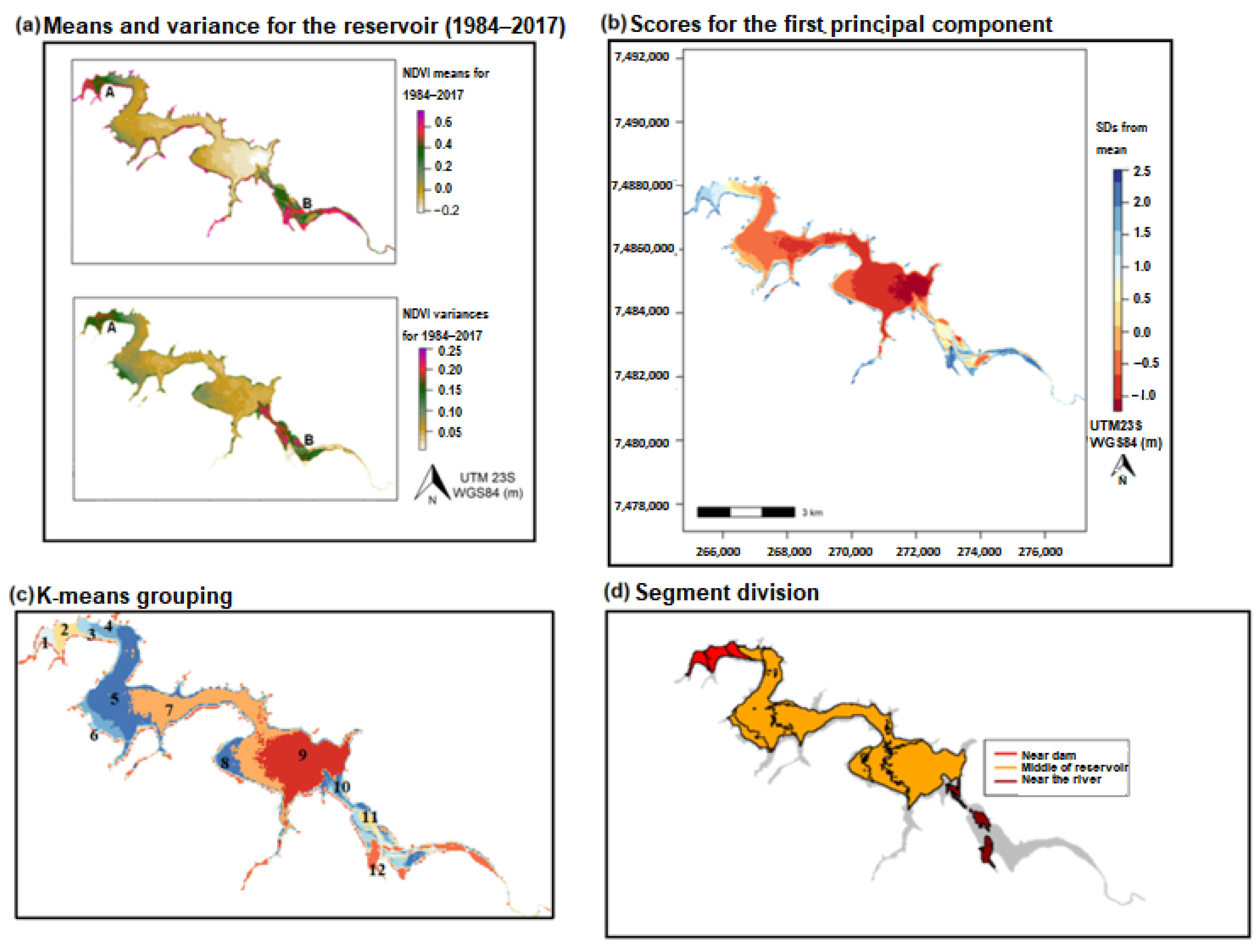
2.2.2. Spatial Segmentation of the Reservoir Based on the Temporal Variance of NDVI

Before performing the spatial segmentation based on the temporal variability of the NDVI, the reservoir was isolated from its surroundings. For that, a vector file of the contour of the reservoir was used to create a water body mask, which was applied to each Landsat image of the reduced collection.

The water body spatial segmentation (Figure 3) is detailed in [7]. This process allows one firstly to map areas of similar temporal correlation and then to define compartments according to the abundance and persistence of macrophytes over time.

The spatial distribution of the NDVI averages calculated from 1985 to 2017 for the Salto Grande reservoir revealed different conditions (Figure 3a). There was a systematic and abundant occurrence of plants close to the dam and where the condition of the river is still maintained (NDVI greater than 0.4) associated with reddish tones, an irregular occurrence of macrophytes (NDVI close to 0.2, with greenish tones), and absence of plants in the central area of the lake (light yellow to white tones). The highest NDVI means were spatially coincident with the largest variances, suggesting that there is a seasonal displacement of plants, influenced by internal and external factors in the water system. Based on this temporal space variability, homogeneous regions of the reservoir were defined as to the occurrence of macrophytes.

T-mode Principal Component Analysis (PCA) was applied to the historical series of NDVI cropped images, and the first principal component (PC1) scores were used to identify the regions of similar temporal correlation (Figure 3b). In the T-mode, the scores of each PC showed spatial patterns defined by strong or weak correlations over time [28] and the proportion of variance of 61% retained in PC1 indicated that NDVI values fluctuated over time and confirmed the variability in the spatial distribution and abundance of macrophytes in the reservoir. Then, the PC1 scores were submitted to unsupervised classification by the k-means algorithm, allowing for the generation of twelve clusters of pixels that presented similar scores (Figure 3c). K-means was used due to the difficulty in defining thresholds that resulted in an appropriate reservoir segmentation considering the NDVI’s spatial variability through time. The mean NDVI of the pixels included in each cluster (called “area”) was calculated, and the NDVI time series was constructed for each area.

The compartments were defined by grouping the areas according to the abundance and persistence of macrophytes over time. Areas 1–3 were considered the “near dam” compartment, areas 4–9 were associated with the “reservoir body”, while areas 10–12 were the “near the river” compartment (Figure 3d).

The spatial segmentation and subsequent sectorization of the reservoir based on the temporal variability of the NDVI was used to analyze the influence of climate variables on the spatial and temporal dispersion of macrophytes in the water body at three levels. For each level of analysis, one or more time series of mean NDVI were generated according to the degree of spatial detail obtained:

−

Reservoir: a single time series of the mean NDVI was used to represent the entire the reservoir.

−

Area: twelve time series of the mean NDVI, calculated for each segmented area.

−

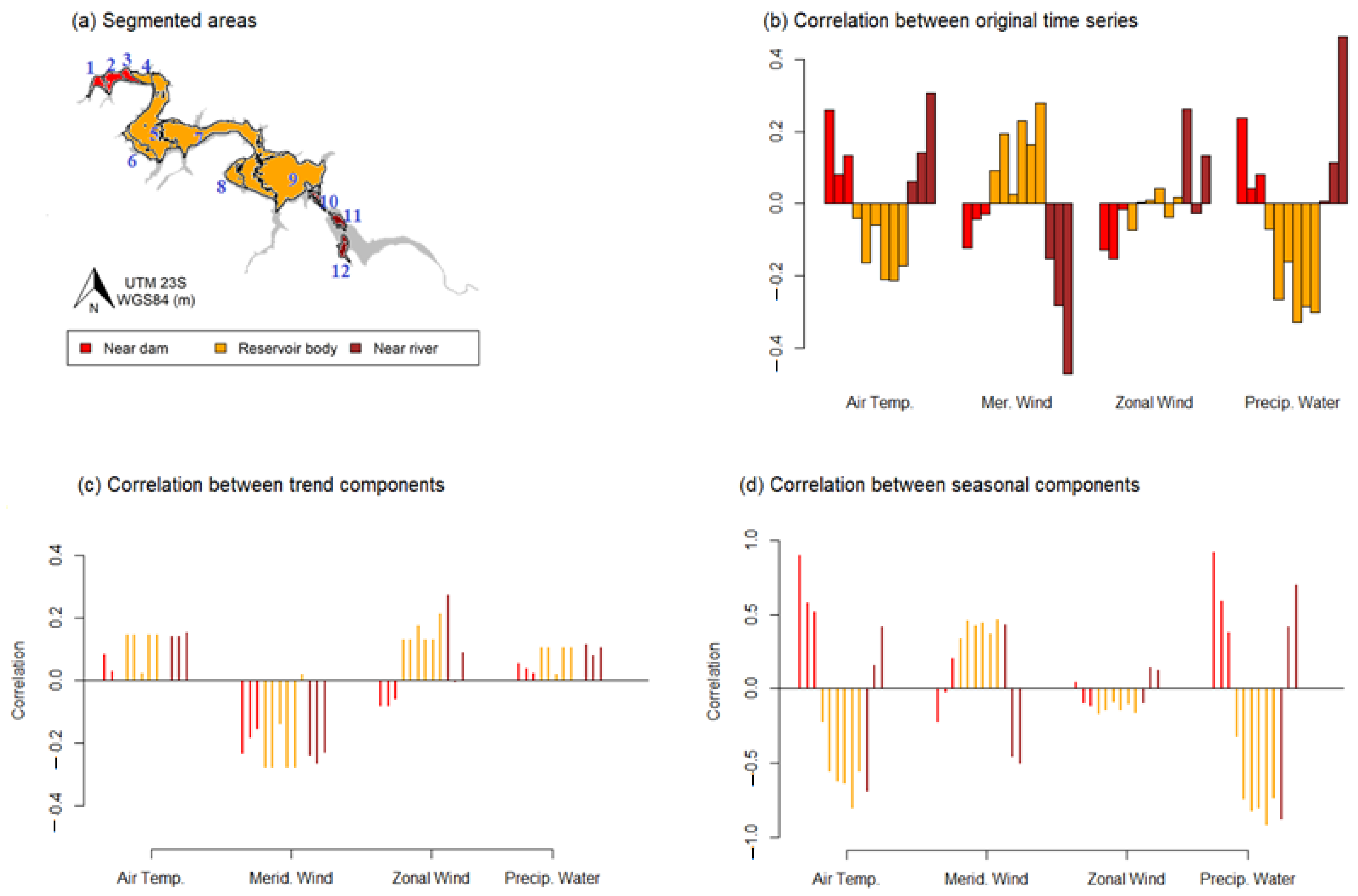
Compartment: three NDVI time series, referring to the mean calculated from the pixels included in the sectors defined as near dam, reservoir body (middle of the reservoir), and near river.

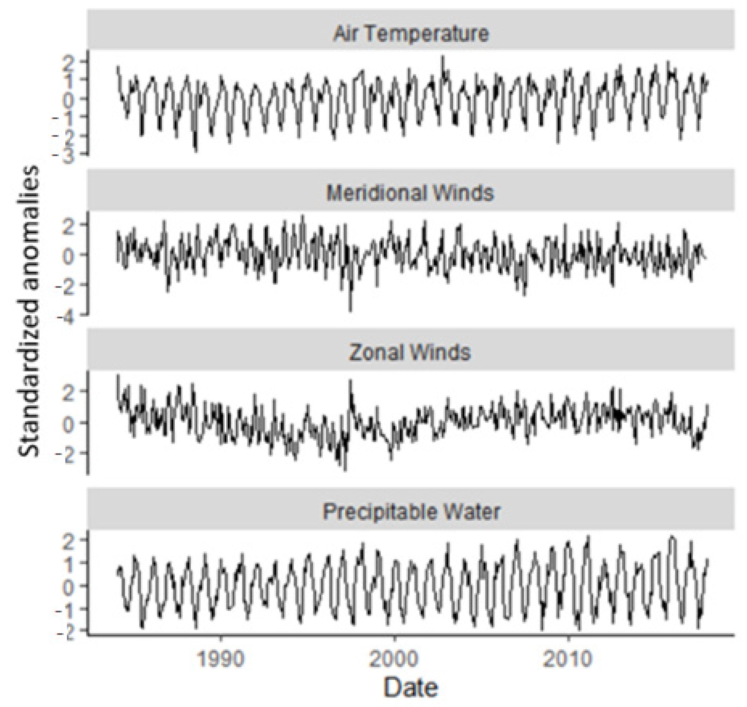
2.2.3. Climate Data Time Series Generation

As there were few weather stations in the region, all far from the reservoir and with different temporal coverage, the NOAA/ESRL datasets were chosen, also because they are freely distributed and one of the most widely used atmospheric assimilation datasets in the world [29]. The NOAA/ESRL data were obtained by reanalysis data, a methodology from the National Centers for Environmental Prediction (NCEP) that integrates various sources of data into a single model through time. The model generation is automated and rigorously monitored, with results being displayed after data gathering and collating at 2.5 by 2.5-degree resolution fields for many variables [30].

When studying the influence of climate changes on hydrology in the Brazilian Pantanal, ref. [18] analyzed the temporal relationship between mean summer rainy days (derived from rainfall data provided by an official network of rain gauge stations) and key climate variables provided by NOAA/ESRL. The authors found the highest linear correlations for precipitable water (r = 0.67) and air temperature (r = 0.59), although the meridional wind component (r = 0.49) was shown to be significant in the study. Considering the unavailability of the data provided for the reservoir area itself, since the nearest climate stations (more than 100 km from the dam) do not continuously cover the entire time period of the analysis, NOAA/ESRL variables were used instead.

For our study, we considered the climate variables air temperature, precipitable water, meridional winds (MW) and zonal winds (ZW), based on the marked seasonal variation in the austral summer (hot and humid) and austral winter (cooler and drier).

Table 1. Climate variables obtained from the NOAA/ESRL website and their characteristics.

Climate Variable	Description	Unit
Air Temperature	Temperature of the air measured at a height of 1.5 m above terrestrial surface.	Celsius (°C)
Precipitable Water	Total water vapor in atmosphere contained in a unitary section column between any two levels of surface, usually the top of atmosphere and terrestrial surface. It is the estimate of potential rain in a determined region.	kg/m3
Meridional and Zonal Wind	The horizontal air movement relative to the terrestrial surface generated by atmospheric pressure gradients. Components of wind are direction, speed, and force it exerts on a determined object: − Meridional wind (v): positive values indicate winds coming from the south. − Zonal wind (u): positive values indicate winds coming from the west.	m/s

summarizes the characteristics of the climate variables considered in our study. All data are available at monthly scale without missing values, at the grid locations for 22°41′24″ to 22°45′36″S and 47°17′24″ to 47°09′57″W at surface level. The data is subjected to a Z-score standardization to make compatible the measurement scales of the different variables, generating the time series shown in Figure 4.

Although a cyclical pattern in the time series of meridional and zonal wind was not explicit, there was a clear seasonal periodicity in the behavior of the air temperature and precipitable water associated with well-defined dry and rainy seasons in the southern hemisphere. Therefore, we assumed that four measurements in the year would be able to capture this seasonal variation, and the monthly data were grouped into quarterly means in order to be compared with the spectral indices obtained for each quarter.

The time series constructed for each of the climate variables and the Landsat NDVI at different levels of generalization are defined in the time interval between 1985 and 2017, all of them with quarterly frequency. Thus, the time series of the climate variables were the same ones used in the analysis of each compartment or segmented area of the reservoir. That is, for area 1 of the reservoir, the same dataset of precipitable water, zonal and meridional winds, and air temperature was used, as was the case for area 12.

2.3. Time Series Analysis

The analysis of the climate variables’ influences on the NDVI was based on the correlation and causality of the components of trend and seasonality of the time series. For the decomposition, the BFAST algorithm (Breaks for Additive Seasonal and Trends; [31]) was applied.

The BFAST algorithm was proposed by [31] and is based on the principle that the estimates of changes are a combination of seasonal changes, gradual and abrupt, the latter being caused by events such as deforestations, urbanizations, floodings, and fires [32]. The BFAST algorithm decomposes the time series in search of gradual and abrupt changes in the seasonal and trend components by looking for breakpoints in observations. Specifically, a ${\mathrm{Y}}_{\mathrm{t}}={\mathrm{y}}_{\mathrm{t}}$ observation for some time $\mathrm{t}$ is modelled as a linear trend component and a harmonic seasonality:

$${\mathrm{Y}}_{\mathrm{t}}={\mathsf{\alpha }}_1+{\mathsf{\alpha }}_2\mathrm{t}+{\displaystyle \sum }_{\mathrm{j}=1}^{\mathrm{k}}{\mathsf{\gamma }}_{\mathrm{j}}\sin \left(\frac{2\mathsf{\pi }\mathrm{jt}}{\mathrm{f}}+{\mathsf{\delta }}_{\mathrm{j}}\right)+{\mathrm{e}}_{\mathrm{t}}$$

(1)

with the unknown parameters being the intercept ${\mathsf{\alpha }}_1$, trend ${\mathsf{\alpha }}_2$, amplitudes ${\mathsf{\gamma }}_{\mathrm{j}}$, and phases (seasonality) ${\mathsf{\delta }}_{\mathrm{j}}$, $\mathrm{j}=1, \dots , \mathrm{k}$. The $\mathrm{f}$ term represents the frequency of the time series, and ${\mathrm{e}}_{\mathrm{t}}$ represents the error for a time $\mathrm{t}$.

The number and positions of breaks in a time series are unknown and must be estimated. The parameter h that specifies the minimum number of observations in a segment must be provided so that the maximum number of breaks will be the ratio between this parameter and the number of observations in time (h/N) [33]. In this study, h = 0.15 was used. The set of breakpoints positions $\left({\mathrm{b}}_1,\dots {\mathrm{b}}_{\mathrm{m}}\right)$ is obtained by a grid search procedure and is optimum when:

$${\mathrm{Y}}_t\left(\widehat{{\mathrm{b}}_1},\dots \widehat{{\mathrm{b}}_{\mathrm{m}}}\right)=\arg {\min }_{\left(\widehat{{\mathrm{b}}_1},\dots \widehat{{\mathrm{b}}_{\mathrm{m}}}\right)}{\displaystyle \sum }_{\mathrm{i}=1}^{\mathrm{N}}{\mathrm{e}}_{\mathrm{i}}^2,$$

(2)

i.e., minimizing the sum of squared residuals. The optimal number of breakpoints is given by the minimum Bayesian Information Criterion (BIC; [34]), expressed by:

$$\mathrm{BIC}=-2\ln \left(\mathrm{L}\right)+\mathrm{Wlog}\left(\mathrm{N}\right),$$

(3)

where L is the likelihood of the model, and W is the number of parameters and is added as a penalty for the model estimation. Although other methods could be used in time series decomposition and analysis, e.g., multivariate linear regression analysis [35], BFAST was chosen as it is a method which simultaneously accounts for variation at seasonal scale while detecting changes in long term trends (gradual interannual and abrupt intraannual changes) that can be masked by seasonal variability. It also requires a minimum amount of processing time and does not require a definition of thresholds [36,37].

The Granger causality technique [38] is used to study if a time series of a specific variable is useful for forecasting another variable. This technique has been used frequently in addressing causality problems, especially in climate systems [39]. If ${\mathrm{X}}_{\mathrm{t}}$ and ${\mathrm{Y}}_{\mathrm{t}}$ are time series, ref. [38] uses the expression “${\mathrm{X}}_{\mathrm{t}}$ Granger-causes ${\mathrm{Y}}_{\mathrm{t}}$” to express the fact that the knowledge of past values of ${\mathrm{X}}_{\mathrm{t}}$ reduces the variance of the errors in forecasting the values of ${\mathrm{Y}}_{\mathrm{t}}$ beyond the variance of the errors which would be made from only the knowledge of past ${\mathrm{Y}}_{\mathrm{t}}$ alone [40]. In mathematical notation, two models are considered, namely, restricted (4) and unrestricted model (5), given, respectively, by:

$${\mathrm{Y}}_{\mathrm{t}}={\mathsf{\alpha }}_0+{\mathsf{\alpha }}_1{\mathrm{Y}}_{\mathrm{t}-1}+{\mathsf{\alpha }}_2{\mathrm{Y}}_{\mathrm{t}-2}+\cdots +{\mathsf{\alpha }}_{\mathrm{p}}{\mathrm{Y}}_{\mathrm{t}-\mathrm{p}}+{ϵ}_{\mathrm{t}}$$

(4)

$${\mathrm{Y}}_{\mathrm{t}}={\mathsf{\beta }}_0+{\mathsf{\alpha }}_1{\mathrm{Y}}_{\mathrm{t}-1}+{\mathsf{\alpha }}_2{\mathrm{Y}}_{\mathrm{t}-2}+\cdots +{\mathsf{\alpha }}_{\mathrm{p}}{\mathrm{Y}}_{\mathrm{t}-\mathrm{p}}+{\mathsf{\beta }}_1{\mathrm{X}}_{\mathrm{t}-1}+\cdots +{\mathsf{\beta }}_{\mathrm{p}}{\mathrm{X}}_{\mathrm{t}-\mathrm{p}}+{\mathsf{\gamma }}_{\mathrm{t}}$$

(5)

with ${\mathsf{\alpha }}_0$ and ${\mathsf{\beta }}_0$ being constants terms, ${\mathsf{\alpha }}_{\mathrm{i}}$ and ${\mathsf{\beta }}_{\mathrm{i}}$ for $\mathrm{i}=1,\dots ,\mathrm{p}$ the unknown parameters, ${ϵ}_{\mathrm{t}}$ and ${\mathsf{\gamma }}_{\mathrm{t}}$ white noise errors, and $\mathrm{p}$ the maximum lag allowed for both models. To test if the restricted estimates are statisically different from the unrestricted estimates, the F-test, $\mathrm{F}=\frac{\left({\mathrm{SSE}}_{\mathrm{r}}-{\mathrm{SSE}}_{\mathrm{u}}\right)/\mathrm{p}}{{\mathrm{SSE}}_{\mathrm{u}}/\left(\mathrm{n}-\mathrm{k}\right)}$ is used, with ${\mathrm{SSE}}_{\mathrm{r}}$ and ${\mathrm{SSE}}_{\mathrm{u}}$ being the sum of squared errors of restricted and unrestricted models, respectively, and $\mathrm{k}$ the number of coefficients in the unrestricted model. If $\mathrm{F}<{\mathrm{F}}_{\mathrm{H},\mathrm{n}-\mathrm{k}}$, ${\mathrm{F}}_{\mathrm{H},\mathrm{n}-\mathrm{k}}$ being the tabulated value of an F-distribution with parameters $\mathrm{p}$ and $\mathrm{n}-\mathrm{k}$, it is concluded that $\mathrm{X}$ does not Granger-cause $\mathrm{Y}$.

For this study, models were investigated by adding lags until significance was observed at the 0.05 level, considering the causality effect of each climate variable on the NDVI according to Equations (6)–(9).

$${\mathrm{NDVI}}_{\mathrm{t}}={\mathsf{\alpha }}_0+{\displaystyle \sum }_{\mathrm{i}=1}^4{\mathsf{\alpha }}_{\mathrm{i}}{\mathrm{NDVI}}_{\mathrm{t}-\mathrm{i}}+{\displaystyle \sum }_{\mathrm{i}=1}^4{\mathsf{\beta }}_{\mathrm{i}}{\mathrm{AT}}_{\mathrm{t}-1}+{\mathsf{ϵ}}_{\mathrm{t}}$$

(6)

$${\mathrm{NDVI}}_{\mathrm{t}}={\mathsf{\alpha }}_0+{\displaystyle \sum }_{\mathrm{i}=1}^4{\mathsf{\alpha }}_{\mathrm{i}}{\mathrm{NDVI}}_{\mathrm{t}-\mathrm{i}}+{\displaystyle \sum }_{\mathrm{i}=1}^4{\mathsf{\beta }}_{\mathrm{i}}{\mathrm{PW}}_{\mathrm{t}-\mathrm{i}}+{\mathsf{ϵ}}_{\mathrm{t}}$$

(7)

$${\mathrm{NDVI}}_{\mathrm{t}}={\mathsf{\alpha }}_0+{\displaystyle \sum }_{\mathrm{i}=1}^4{\mathsf{\alpha }}_{\mathrm{i}}{\mathrm{NDVI}}_{\mathrm{t}-\mathrm{i}}+{\displaystyle \sum }_{\mathrm{i}=1}^4{\mathsf{\beta }}_{\mathrm{i}}{\mathrm{MW}}_{\mathrm{t}-\mathrm{i}}+{\mathsf{ϵ}}_{\mathrm{t}}$$

(8)

$${\mathrm{NDVI}}_{\mathrm{t}}={\mathsf{\alpha }}_0+{\displaystyle \sum }_{\mathrm{i}=1}^4{\mathsf{\alpha }}_{\mathrm{i}}{\mathrm{NDVI}}_{\mathrm{t}-\mathrm{i}}+{\displaystyle \sum }_{\mathrm{i}=1}^4{\mathsf{\beta }}_{\mathrm{i}}{\mathrm{ZW}}_{\mathrm{t}-\mathrm{i}}+{\mathsf{ϵ}}_{\mathrm{t}}$$

(9)

with $\mathrm{NDVI}$ being NDVI values, $\mathrm{AT}$ the values for air temperature, $\mathrm{PW}$ the values for precipitable water, $\mathrm{MW}$ the meridional wind values, and $\mathrm{ZW}$ the zonal wind values, all for $\mathrm{t}=1984, \dots , 2017$; $\mathsf{\alpha }$ and $\mathsf{\beta }$ are the unknown parameters estimated, and $\mathsf{ϵ}$ represents the white noise errors.

Prior to the application of the models, the Augmented Dickey–Fuller test [41] was used to verify the stationarity of the time series. Since all time series were stationary, the BIC criterion was used to add lags to the models in order to verify the climatic variables (and their lagged values, along with the NDVI and its lagged values), and this helped in the NDVI prediction. Thus, the Granger causality test was applied by adding terms (climate variables and their lagged values) to the NDVI model.

The influence of climate variables on NDVI was evaluated in terms of trend and seasonality, considering the entire reservoir and, individually, for compartments and each of the twelve areas of homogeneous temporal variability. All these processes were implemented in the software R for statistical computing [42] using Rgdal, raster, bfast, and psych packages.

3. Results

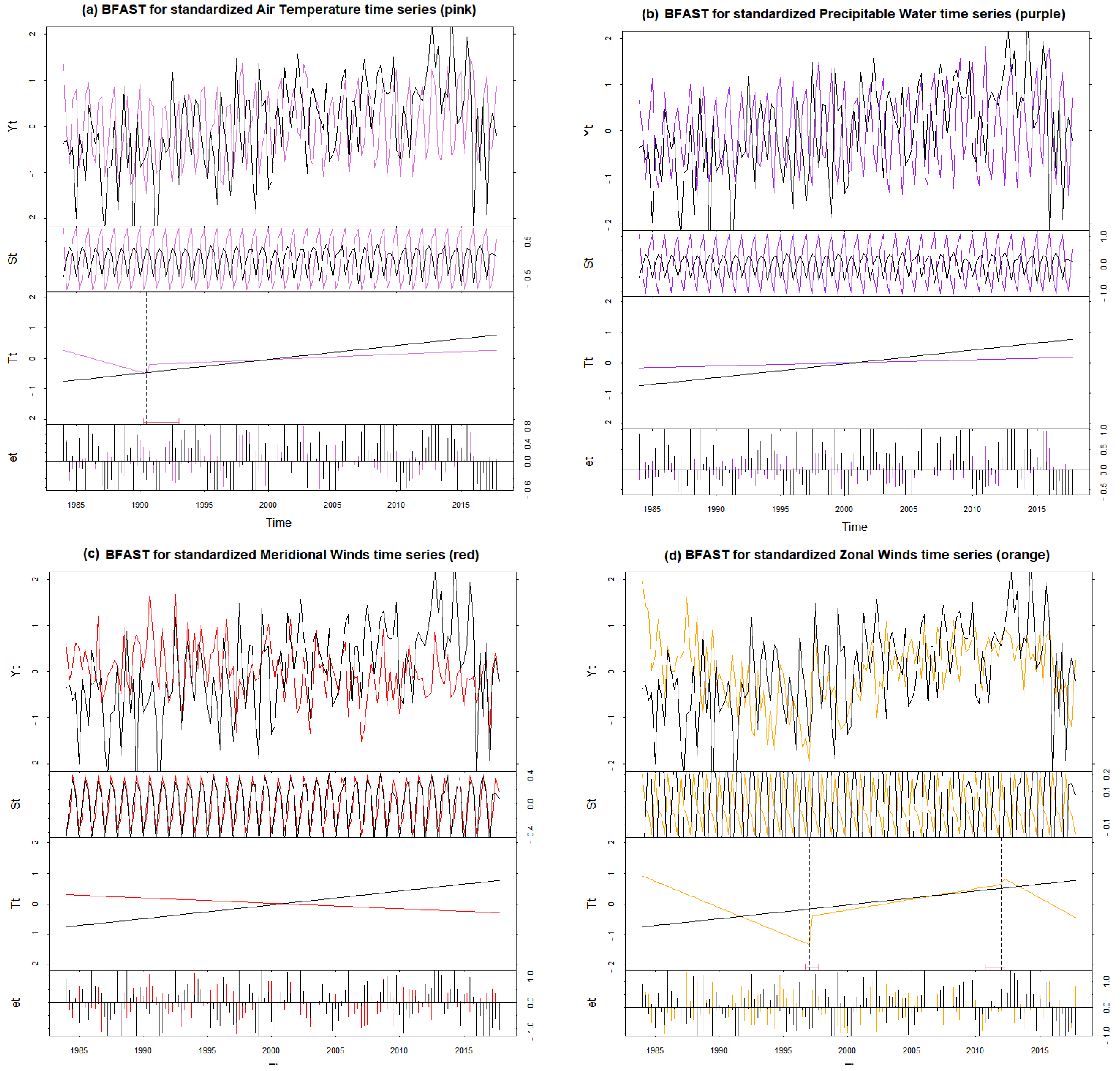
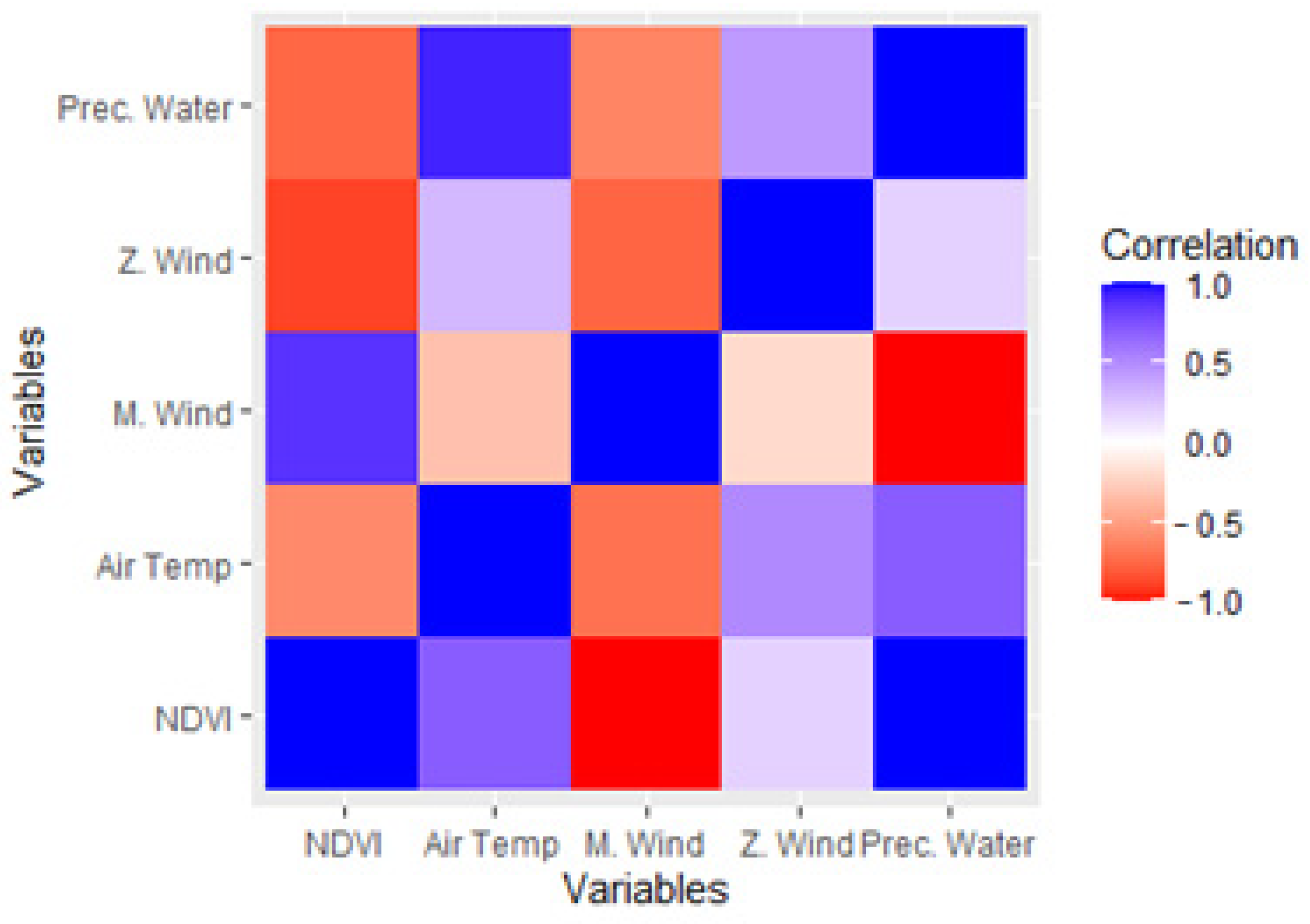
3.1. Temporal Relationship of Climatic Variables and NDVI of the Reservoir

From the data provided by NOAA/ESRL, the quarterly time series constructed for the climate variables were compared with the mean NDVI time series for the entire reservoir (Figure 5). The mean values represented in the original NDVI (black) and air temperature (pink) time profiles (Figure 5a) made up the first panel (${\mathrm{Y}}_{\mathrm{t}}$) and pointed to greater variability of both variables, mainly NDVI associated with the occurrence of macrophytes in the reservoir. A markedly cyclical pattern was perceived in the time series, although the seasonality component (${\mathrm{S}}_{\mathrm{t}}$) indicated a shift of more than six months between the peaks of the two variables. In terms of trend (${\mathrm{T}}_{\mathrm{t}}$), while the air temperature showed a very small increase over time, after a reversal in the downward trend in the early 1990s, the growth of macrophytes in the reservoir was continuous and more pronounced.

The quarterly time series of precipitable water (Figure 5b, purple) had a similar behavior to that of air temperature when compared to the time series of the reservoir NDVI, in terms of seasonality (${\mathrm{S}}_{\mathrm{t}}$). The trend of increasing precipitation was very small over time, in contrast to the sharp increase in NDVI.

Although the original time series of NDVI and meridional wind (Figure 5c, red) resulted in very different profiles, the seasonality pattern was similar, with higher and lower coincident values for both variables. Meridional wind showed a slightly decreasing trend (${\mathrm{T}}_{\mathrm{t}}$), despite the difficulty in interpreting this scenario, since the value of this variable incorporates speed, force, and direction that is associated with the signal (positive for winds coming from the south).

Zonal Wind is another climate variable that is difficult to interpret due to the complex composition of its value (speed and force, winds from the west define positive signs). It shows two break points in its trend (Figure 5d, orange). Events with repercussions in 1997 altered the downward trend in the values of this variable and, later in 2012, reversed the upward trend for a further fall in the values.

The temporal correlation between each climate variable and the mean NDVI obtained for the entire reservoir was also analyzed by comparing, in addition to the original time series, the components of trend and seasonality separately. The cross-correlation of ${\mathrm{Y}}_{\mathrm{t}}$, i.e., between the NDVI time series and the climate variables time series, were obtained at 5% significance level. Correlating the mean NDVI calculated for the entire reservoir with air temperature, precipitable water, and zonal and meridional winds resulted in the values of −0.0678, −0,1951, 0.0754, and 0.0491, respectively, indicating that low correlation values predominated in the original time series.

The correlations between the NDVI time series and each climate variable, individually in terms of trend and seasonality, had quite different behaviors for these time series components (Figure 6). The correlation was low for zonal winds (0.1947), which showed two break points, followed by a change in trend. For time series seasonal components, high positive and negative correlations were also observed (−0.5958, 0.875, −0.8835, and −0.7551) when comparing mean NDVI with the seasonality of air temperature, meridional winds, zonal winds, and precipitable water, respectively.

In the study of the causality of each climate variable on the mean NDVI of the reservoir, the Granger technique was applied using up to the fourth temporal lag of the climate variables (

Table 2. Granger causality (GC) p-values between the climate variables and reservoir mean NDVI for maximum lag obtained by Bayesian Information Criterion (BIC).

Variable Cause	Lags Used	Variable GC NDVI p (<F)
Air Temperature	1, 2, 3, 4	0.0001
Meridional Wind	1	0.0006
Zonal Wind	1	0.0030
Precipitable Water	1, 2, 3, 4	0.0086

). Where no single root presence was detected, no differentiation was necessary for these time series. The models were defined by adding lags in each variable until p (<F) < 0.05, and Bayesian Information Criterion (BIC) selected to inspect the model at a significance level of 5%.

The air temperature and precipitable water time series needed four lags’ quarters behind to reach the significance level of 0.05 and helped to explain the future state of the NDVI for the entire reservoir (Table 2). In the case of time series of the variables meridional and zonal wind, one lag was enough to help in predicting the future state of the reservoir mean NDVI.

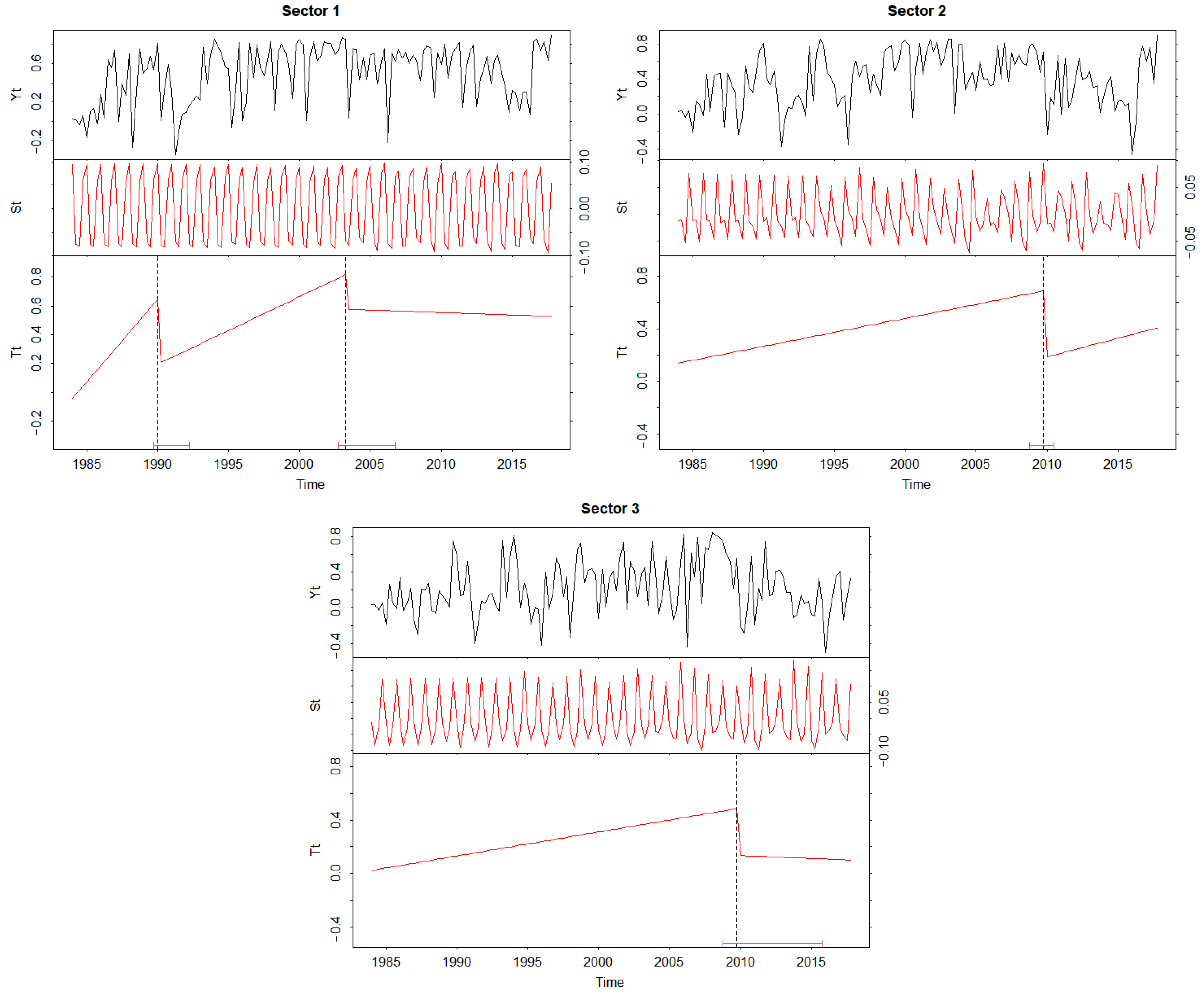
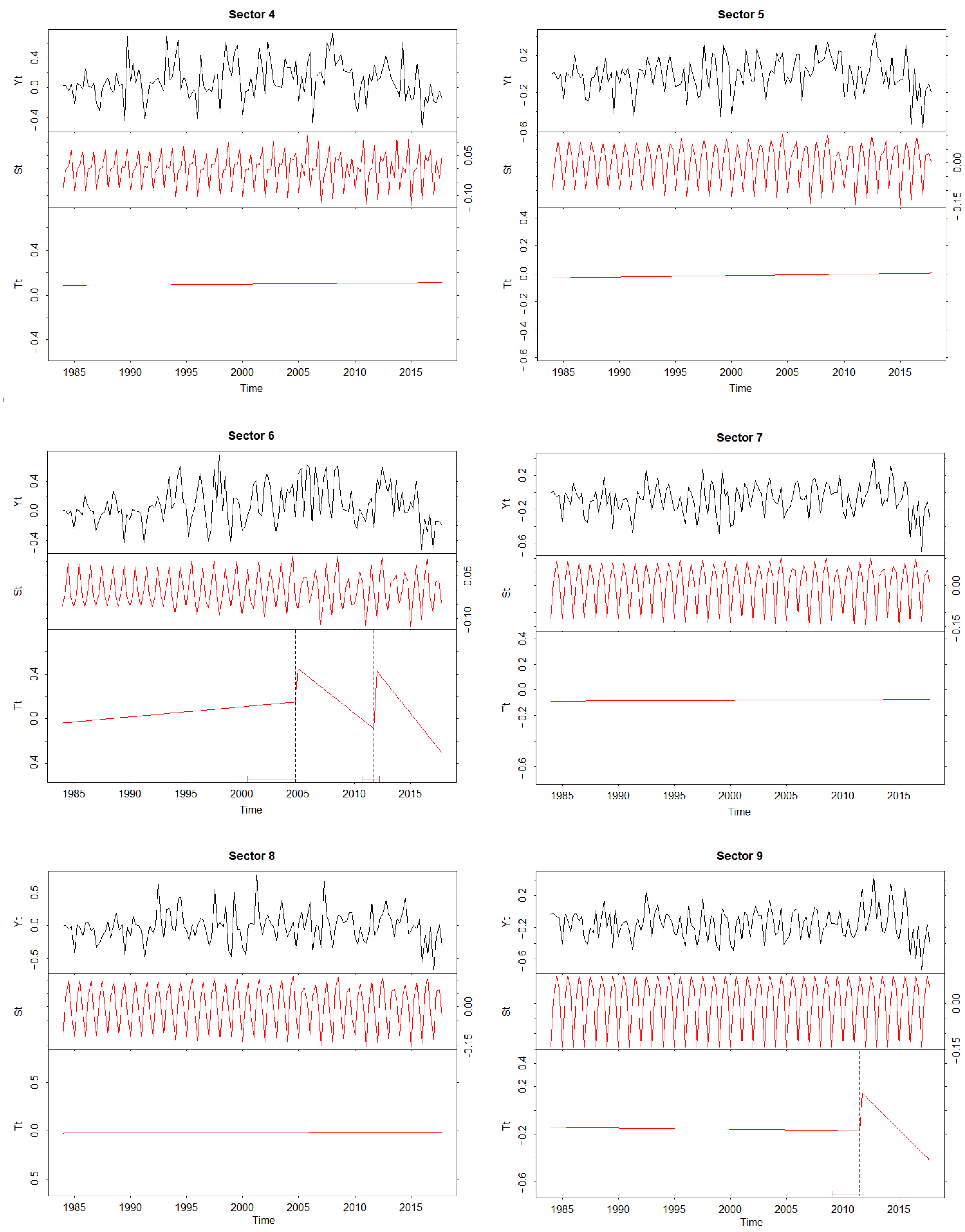
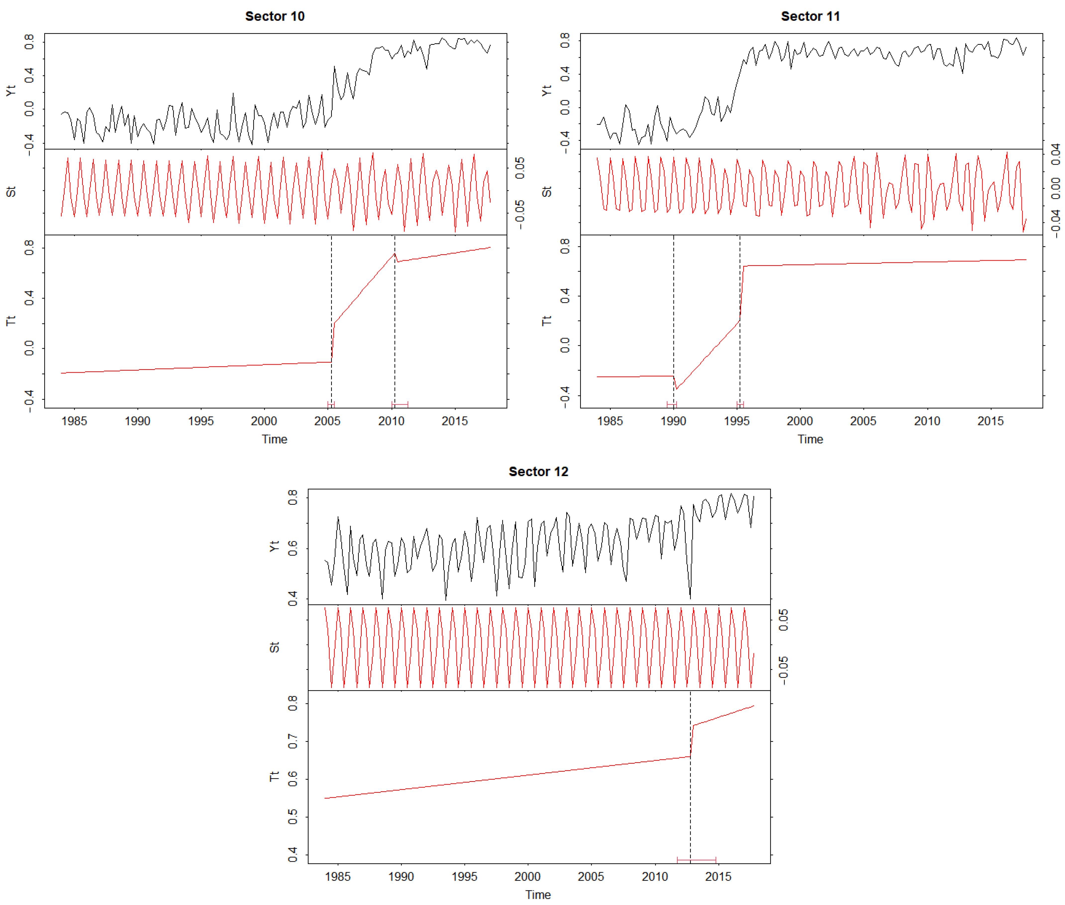
3.2. Influence of Climate Variables on NDVI Spatial Variability over Time

To analyze the influence of climatic variables on the macrophyte’s occurrence in different sectors of the reservoir over time, both the compartments that formed the water body and the twelve segmented areas were considered. In order to show the spatiotemporal variability of the NDVI and, therefore, the occurrence of macrophytes in the reservoir, the NDVI time series of the segmented areas were presented, grouped according to the compartment they represent. Figure 7 shows the time series and respective seasonality and trend components of the segmented areas that comprised the near dam compartment. Figure 8 and Figure 9 constitute the time series of the segmented areas of the reservoir body and near river compartments, respectively.

In the near dam (Figure 7) and near river (Figure 9) compartments, all segmented areas defined, in some periods, maximum NDVI values compatible with abundant vegetation, while in the reservoir body, maximum NDVI values close to 0.2 were predominant. Reservoir body areas 4, 6, and 8, located on the southwest margin of the water body, reached NDVI values of the order of 0.4 or 0.5 in some periods, but only area 6 defined breakpoints in the trend. On the other hand, the segmented areas of the near dam compartment, such as the near river, had at least one breakpoint.

For the spatiotemporal analysis of the influence of climate variables on NDVI of the specific sectors of the water body, a procedure similar to that for the entire reservoir was adopted.

Table 3. Correlation between the time series (original, trend, and seasonality components) of the mean NDVI and climate variables per reservoir compartment.

Compartment	Time Series	Climate Variables
		Air Temperature	Meridional Wind	Zonal Wind	Precipitable Water
Near dam	Original	0.1641	−0.0709	−0.1208	0.1194
	Trend	0.0394	−0.2068	−0.0369	0.0463
	Seasonality	0.7695	−0.0175	−0.0540	0.7240
Reservoir body	Original	−0.1902	0.2356	0.0163	−0.3120
	Trend	0.1461	−0.2759	0.1291	0.1039
	Seasonality	−0.5950	0.4526	−0.1424	−0.7694
Near river	Original	0.1625	−0.3125	0.1318	0.1474
	Trend	0.1621	−0.2870	0.1614	0.1072
	Seasonality	0.0972	−0.4898	0.1429	0.4000

indicates the correlations calculated between the time series of the mean NDVI per reservoir compartment and climate variables.

The correlations between the original time series of the mean NDVI and each climate variable remained low for the three compartments, as well as the trend components, which did not reach 0.3, regardless of the compartment or climate variable considered. However, the cross correlations between the components of seasonality showed that the persistence of macrophyte banks close to the dam had a cyclical behavior positively correlated with fluctuations in air temperature (0.7695) and precipitable water (0.724). This did not occur near the river, which had a negative correlation of less than 0.5 with meridional wind. In the middle of the reservoir, the highest correlation of the seasonal behavior of the mean NDVI was observed in the variable precipitable water (−0.7694).

To analyze the temporal and seasonal influence of the climate variables on the mean NDVI calculated for each of the twelve areas segmented by the k-means algorithm (Figure 10a), the cross-correlations were calculated considering initially the original time series, shown in Figure 10b, by means of bar plots. By decomposing each NDVI time series into trend and seasonality of each NDVI segmented area, and correlating with the climate variables values, the values shown in Figure 10c,d were obtained for the areas and represented by lines. In these three graphs, each bar or line, representing areas 1 to 12, is associated with the “near dam”, “reservoir body”, and “near river” compartments and labelled by colors.

The correlation values between the original time series of the climate variables and the NDVI by area were all less than 0.5, but all, except zonal winds, allowed the three compartments of the reservoir to be discriminated. Air temperature and precipitable water had similar correlation behaviors. They were positively correlated with NDVI in the near dam and near river sectors and negatively correlated with NDVI in the reservoir body. Meridional wind was negatively correlated with NDVI in these sectors and positively correlated in the reservoir body. The zonal wind showed no correlation with NDVI in the reservoir body. The highest negative and positive correlations occurred for meridional wind and precipitation, respectively, both in the near river compartment. Aside from the zonal wind variable, all others clearly produced correlation patterns with NDVI.

The trend component over time resulted in a low correlation between the mean NDVI results of the segmented areas and the climate variables, none of which exceeded 0.3 (Figure 10c). However, the greater correlations obtained for the seasonality component in the segmented areas (Figure 10d) indicated that the spatial dispersion and persistence of aquatic plants in specific locations of the reservoir are related to the cyclical variations of precipitation, air temperature, and winds from the south. Both precipitation and temperature variables that defined high correlations with the NDVI for the seasonality component had a similar behavior for the three sectors of the reservoir, namely, positive correlations in the sectors near the dam and in the environment under the influence of the river. Nonetheless, the seasonal variability in the occurrence of macrophytes in the reservoir body had negative correlations with these variables (all greater than 0.5, except for area 4). Winds from the south had positive correlations and were close to 0.5 with the areas defined as the reservoir body, indicating that the occurrence of macrophyte banks in this sector is influenced by the seasonal behavior of these winds. Zonal wind had very little influence in all sectors.

In the analysis of causality for compartments (

Table 4. Granger causality p-values and number of lags used for the models between the climate variables and mean NDVI of each compartment of the reservoir: near dam (I), reservoir body (II), and near river (III). Bolded are values that are statistically insignificant.

Compartment	Air Temperature		Meridional Winds		Zonal Winds		Precipitable Water
	Lags	p-Value	Lags	p-Value	Lags	p-Value	Lags	p-Value
I	1, 2, 3, 4	0.007	1	0.007	1	0.04	1, 2, 3, 4	0.03
II	1, 2, 3, 4	0.000	1	0.008	1	0.03	1, 2, 3, 4	0.04
III	1, 2, 3, 4	0.05	1, 2, 3, 4	0.55	1, 2, 3, 4	0.88	1, 2, 3, 4	0.02

p-value > 0.05 is not significant: The variable does not Granger-cause NDVI for this area.

) and segmented areas (

Table 5. Granger causality p-values and number of lags used for the models relating climatic variables and NDVI time series of each segmented area of the reservoir.

	Air Temperature		Meridional Wind		Zonal Wind		Precipitable Water
	Lags	p-Value	Lags	p-Value	Lags	p-Value	Lags	p-Value
Area 1	1, 2, 3, 4	0.01	1, 2, 3	0.001	1, 2, 3, 4	0.05	1, 2, 3, 4	0.003
Area 2	1, 2, 3, 4	0.177	1, 2, 3	0.047	1	0.04	1, 2, 3, 4	0.339
Area 3	1, 2, 3, 4	0.004	1, 2, 3	0.016	1, 2, 3, 4	0.647	1, 2, 3, 4	0.009
Area 4	1, 2, 3, 4	0.015	1, 2, 3, 4	0.146	1, 2, 3, 4	0.839	1, 2, 3, 4	0.206
Area 5	1, 2, 3, 4	0.000	1	0.036	1, 2, 3, 4	0.240	1, 2, 3, 4	0.001
Area 6	1, 2, 3, 4	0.084	1	0.023	1, 2, 3, 4	0.250	1, 2, 3, 4	0.068
Area 7	1, 2, 3, 4	0.000	1	0.003	1	0.002	1, 2, 3, 4	0.000
Area 8	1, 2, 3, 4	0.000	1	0.006	1, 2, 3, 4	0.004	1, 2, 3, 4	0.000
Area 9	1, 2, 3, 4	0.000	1	0.035	1	0.030	1, 2, 3, 4	0.000
Area 10	1, 2, 3, 4	0.008	1, 2, 3, 4	0.008	1	0.021	1, 2, 3, 4	0.014
Area 11	1, 2, 3, 4	0.263	1, 2, 3, 4	0.7177	1, 2, 3, 4	0.781	1, 2, 3, 4	0.086
Area 12	1, 2, 3, 4	0.000	1, 2, 3, 4	0.009	1, 2, 3, 4	0.652	1, 2, 3, 4	0.000

p-value > 0.05, in bold, is not significant: The variable does not Granger-cause NDVI for this area.

), the same parameters and thresholds used in the analysis of the entire reservoir were adopted. Thus, the Granger technique was applied using up to the fourth temporal lag to evaluate the causality of each climatic variables on the mean NDVI for these sectors. The models were defined by adding lags in each variable until p (<F) < 0.05 and BIC selection to inspect the model considering a significance level of 5%. The climate variables considered (air temperature, meridional winds, zonal winds and precipitable water) were considered, the number of lags used, and the p-value obtained from the models that met the 5% significance level until the fourth lag of each climate variable was reached.

For the three defined compartments, air temperature and precipitable water required four lags to reach the 0.05 significance level. In the case of meridional and zonal winds, only one lag was sufficient to help predict future states of the NDVI for compartments located near the dam and in the reservoir body. In the near river compartment, still under the lotic effect, even adding four lags to the models did not make the p-value significant for meridional and zone wind, indicating that these variables did not influence the future NDVI values. Table 5 presents the number of lags needed to reach the significance level of 5%, as well as the p-value obtained from the models of air temperature, meridional wind, zonal wind, and precipitable water on the NDVI time series for each segmented area of the reservoir.

When analyzing segmented areas of the reservoir (Table 5), even within the same compartment, it was found that for area 2 (near dam) a significance level of 0.05 was not reached in the causality models, even with the maximum number of lags for air temperature and precipitable water. Only in the largest segmented areas located in the reservoir body (5 to 9) did meridional wind Granger-cause NDVI with only the knowledge of one lag. However, in the narrowest and most confined areas, located near the dam or near the river, it took at least three lags to reach the 0.05 significance level. Even the knowledge of the four past lags was not enough to define significant models for this climate variable in areas 4 and 11.

The influence of zonal wind on the NDVI is not related to the position of the segmented areas in the context of the reservoir (oriented in the east–west direction). None of the climate variables Granger-caused NDVI in area 11, located in the compartment under lotic influence (near river).

4. Discussion

In dealing with the influence of climatic variables in the spatiotemporal dynamics of macrophytes in a eutrophic reservoir, this study explores how their effects manifest over time in the entire reservoir, then in the compartment level and in homogeneous areas defined by the temporal variability of aquatic vegetation occurrence. This multiscale approach considers a prior definition of the segmented areas but effectively investigates the incorporation of the climate temporal variability at each level of spatial generalization.

When considering the reservoir, the comparison between the NVDI time series and the time profile of each climatic variable shows that the accentuated cyclical pattern of air temperature and precipitable water is noticeable even in the original profiles of these variables. The seasonality component, however, better captures this cyclicity, even in the meridional and zonal wind data. Regarding the general behavior of these variables over time, meridional wind presents a decreasing trend with no breakpoints, while precipitable water also presents an increasing trend with no breakpoints.

Air temperature shows a trend break in 1990, but zonal wind, however, presents two breakpoints in its trend component: one in 1997 and another in 2012. The time intervals between 1990–1993 and 1997–1998 were periods of strong El Niño occurrence, and 2012 was a period of La Niña [43]. Thus, the breakpoint in air temperature in the early 1990s may be associated with this event that increased the temperature in tropical western areas and weakened easterly winds near the Americas [44]. None of these episodes influence the growing tendency for macrophytes to occur in the reservoir.

The correlations between each climate variable and mean NDVI of the entire reservoir indicate that variations in occurrence and, eventually, heterogeneous distribution of macrophytes are related to climate fluctuations, both in trend and seasonality. However, the low correlations between the original time series against high correlations in the trend and seasonality components individually confirm our perception of the need to monitor only specific regions of the reservoir over time.

Deepening the analysis of specific regions of the reservoir, first for the three compartments and then for the twelve areas segmented, it is found that the highest correlations are now defined for the seasonality component. This occurs mainly for the climate variables air temperature and precipitable water, but not in all segmented areas and compartments. On the other hand, the correlations obtained between the trend components of the compartments and the segmented areas define low values, different from the correlation of trends for the whole reservoir, which are higher for three of the climate variables, except for zonal wind.

These minor correlations in the trend are partially explained by the breakpoints recorded in the behavior of this component of the NDVI time series on specific areas of the reservoir (Figure 7, Figure 8 and Figure 9). These breaks are due to human interventions in the reservoir in the form of removal of aquatic vegetation in the areas close to the dam and in small areas in the vicinity of population settlements on the right bank of the water body. They can also be attributed to variations in the rate of release of effluents into the water from domestic sewers originating from Campinas and nearby municipalities, as well as agricultural activities near the Atibaia river [7].

The analysis of the correlations between the time series at the compartment level show that it is the effect of seasonality that most influences the occurrence of macrophytes. Thus, the persistence in the occurrence of macrophyte banks in the compartment near the dam has cyclical fluctuations positively correlated with temperature and precipitation, which does not happen in the compartment near the river, in which the constant presence of macrophytes is not influenced by these climate variables.

As expected, the correlations resulting from the analysis of specific reservoir areas for the trend results in values that are almost always lower. On the one hand, the correlations between the mean NDVI of each segmented area based on the temporal variability of the occurrence of macrophytes confirm the initial evidence outlined in the compartment level analysis; it is the seasonality components of the time series that are correlated. On the other hand, even resulting in lower values, the correlations between the original time series allow for better discrimination of the three compartments of the reservoir when considering the influence of temperature, precipitation, and winds from the south.

Moreover, relationships between NDVI and climate factors are also highlighted when not only trend and seasonality are correlated in specific locations of the area with the climatic profiles, but also when incorporating these variables to the NDVI time series through a Granger-causality model. Thus, for the entire reservoir, the knowledge of past values of air temperature and precipitable water (in this case, four quarters behind) are useful in explaining the future state of NDVI over and above knowledge of the history of NDVI, while for meridional and zonal wind, knowledge of only one lag helped in predicting future NDVI.

The same scenario reported for the entire reservoir is observed in the “near dam” and “reservoir body” compartments. However, the meridional and zonal Wind do not influence the NDVI of the “near river” sector, even when four lags are added to the model. It was also observed that some areas do not reach the level of significance expected for random models, even for four lags and within the same compartment. This situation is evident for zonal wind, mainly in the reservoir body, in contrast to meridional wind in the same compartment, Granger-caused NDVI with the knowledge of just one lag in wider open areas of the water body. Supposedly, variables that use four lags to define the causality model (temperature, precipitation) better capture NDVI’s seasonal variations.

In general terms, it is found that variations in macrophyte occurrence are mainly related to fluctuations in air temperature, precipitable water, and meridional wind, both in trends and seasonality. However, it is the cyclical variation of these climate variables that defined the spatial distribution of macrophytes in the reservoir. Increases in air temperature and precipitable water lead to the accumulation of macrophytes in the extreme sectors of the reservoir (near dam and under the influence of the river), while meridional wind is associated with the dispersion of aquatic vegetation in the reservoir body. Furthermore, past observations of climate variables can be important to describe and predict the persistence and macrophyte dispersion in the reservoir.

5. Conclusions

To assess the influence of climatic factors on the spatiotemporal dynamics of macrophytes in eutrophic reservoirs, it was assumed that the dispersion of aquatic vegetation has its rhythm and persistence influenced by climatic conditions. It is, therefore, a phenomenon that must be studied for a long period of time. Considering the current availability of the historical series of Landsat images, it was possible to follow the dynamic behavior of the occurrence of aquatic macrophyte banks in a highly anthropized reservoir and confirm the hypothesis that the rhythm of the spatial distribution of this vegetation is influenced by climate fluctuations.

To evaluate this proposition, a time series analysis approach based on attributes extracted from Landsat images and climate data was designed to investigate the Salto Grande reservoir located in Brazil as a case study. The influence of weather conditions was evaluated through joint analyses of NDVI time series and climate oscillation time profiles, constructed from the NOAA historical records of the Air Temperature, Meridional and Zonal Wind, and Precipitable Water. The information provided by the indices and climate variables considering the time series decomposition approach highlighted seasonal patterns in the long-term analysis and the importance of these variables in the macrophytes’ spatiotemporal analysis.

The study revealed that the monitoring of macrophyte overgrowth in reservoirs can benefit from the integration of the NDVI time series images with climate data. Assessing the relationship between climate variables and the spatiotemporal behavior of macrophytes is essential in forecasting models and provides useful information for the management of eutrophic reservoirs subject to systematic macrophyte infestations. Awareness of when and where the control should be applied is a key to making the management process more efficient, as well as identifying the most sustainable type of management for each situation.

References

1. Luo, J.; Li, X.; Ma, R.; Li, F.; Duan, H.; Hu, W.; Qin, B.; Huang, W. Applying remote sensing techniques to monitoring seasonal and interannual changes of aquatic vegetation in Taihu Lake, China. Ecol. Indic. 2016, 60, 503–513. [Google Scholar] [CrossRef]
2. Dar, N.A.; Pandit, A.K.; Ganai, B.A. Factors affecting the distribution patterns of aquatic macrophytes. Limnol. Rev. 2014, 14, 75–81. [Google Scholar] [CrossRef] [Green Version]
3. Lettenmaier, D.P.; Alsdorf, D.; Dozier, J.; Huffman, G.J.; Pan, M.; Wood, E.F. Inroads of remote sensing into hydrologic science during the WRR era. Water Resour. Res. 2015, 51, 7309–7342. [Google Scholar] [CrossRef]
4. Shekede, M.D.; Kusangaya, S.; Schmidt, K. Spatio-temporal variations of aquatic weeds abundance and coverage in Lake Chivero, Zimbabwe. Phys. Chem. Earth Parts A/B/C 2008, 33, 714–721. [Google Scholar] [CrossRef]
5. Silva, T.S.F.; Costa, M.P.F.; Melack, J.M. Spatial and temporal variability of macrophyte cover and productivity in the eastern Amazon floodplain: A remote sensing approach. Remote Sens. Environ. 2010, 114, 1998–2010. [Google Scholar] [CrossRef]
6. Tena, A.; Vericat, D.; Gonzalo, L.E.; Batalla, R.J. Spatial and temporal dynamics of macrophyte cover in a large regulated river. J. Environ. Manag. 2017, 202, 379–391. [Google Scholar] [CrossRef]
7. Coladello, L.F.; Galo, M.L.B.T.; Shimabukuro, M.H.; Ivánová, I.; Awange, J. Macrophytes’ abundance changes in eutrophicated tropical reservoirs exemplified by Salto Grande (Brazil): Trends and temporal analysis exploiting Landsat remotely sensed data. Appl. Geogr. 2020, 121, 102242. [Google Scholar] [CrossRef]
8. Jacquin, A.; Sheeren, D.; Lacombe, J.-P. Vegetation cover degradation assessment in Madagascar savanna based on trend analysis of MODIS NDVI time series. Int. J. Appl. Earth Obs. Geoinf. 2010, 12, S3–S10. [Google Scholar] [CrossRef] [Green Version]
9. Agutu, N.; Awange, J.; Zerihun, A.; Ndehedehe, C.; Kuhn, M.; Fukuda, Y. Assessing multi-satellite remote sensing, reanalysis, and land surface models’ products in characterizing agricultural drought in East Africa. Remote Sens. Environ. 2017, 194, 287–302. [Google Scholar] [CrossRef] [Green Version]
10. Awange, J.L.; Saleem, A.; Sukhadiya, R.; Ouma, Y.O.; Hu, K. Physical dynamics of Lake Victoria over the past 34 years (1984–2018): Is the lake dying? Sci. Total Environ. 2019, 658, 199–218. [Google Scholar] [CrossRef]
11. Morgen, B.; Awange, J.L.; Saleem, A.; Hu, K. Understanding vegetation variability and their ‘‘hotspots’’ within Lake Victoria Basin (LVB: 2003–2018). Appl. Geogr. 2020, 122, 102238. [Google Scholar] [CrossRef]
12. Powell, S.; Jakeman, A.; Croke, B. Can NDVI response indicate the effective flood extent in macrophyte dominated floodplain wetlands? Ecol. Indic. 2014, 45, 486–493. [Google Scholar] [CrossRef]
13. Phiri, M.; Shiferaw, Y.A.; Tesfamichael, S.G. Biome-level relationships between vegetation indices and climate variables using time-series analysis of remotely-sensed data. GIScience Remote Sens. 2020, 57, 464–482. [Google Scholar] [CrossRef]
14. Fusilli, L.; Collins, M.O.; Laneve, G.; Palombo, A.; Pignatti, S.; Santini, F. Assessment of the abnormal growth of floating macrophytes in Winam Gulf (Kenya) by using MODIS imagery time series. Int. J. Appl. Earth Obs. Geoinf. ITC J. 2013, 20, 33–41. [Google Scholar] [CrossRef]
15. Villa, P.; Pinardia, M.; Bolpagnib, R.; Gillierc, J.M.; Zinked, F.N.; Bresciani, M. Assessing macrophyte seasonal dynamics using dense time series of medium resolution satellite data. Remote Sens. Environ. 2018, 216, 230–244. [Google Scholar] [CrossRef]
16. Eckert, S.; Hüsler, F.; Liniger, H.; Hodel, E. Trend analysis of MODIS NDVI time series for detecting land degradation and regeneration in Mongolia. J. Arid Environ. 2015, 113, 16–28. [Google Scholar] [CrossRef]
17. Santos, M.; Melendez-Pastor, I.; Navarro-Pedreño, J.; Koch, M. Assessing water availability in Mediterranean regions affected by water conflicts through MODIS data time series analysis. Remote Sens. 2019, 11, 1355. [Google Scholar] [CrossRef] [Green Version]
18. Bergier, I.; Assine, M.L.; McGlue, M.M.; Alho, C.R.J.; Silva, A.; Guerreiro, R.L.; Carvalho, J.C. Amazon rainforest modulation of water security in the Pantanal wetland. Sci. Total Environ. 2018, 619–620, 1116–1125. [Google Scholar] [CrossRef]
19. Wang, G.; Zhang, X.; Zhang, S. Performance of three reanalysis precipitation datasets over the Qinling-Daba mountains, Eastern Fringe of Tibetan Plateau, China. Adv. Meteorol. 2019, 2019, 7698171. [Google Scholar] [CrossRef] [Green Version]
20. Awange, J. Lake Victoria Monitored from Space; Springer: Berlin/Heidelberg, Germany, 2021. [Google Scholar] [CrossRef]
21. Awange, J. The Nile Waters Weighed from Space; Springer: Berlin/Heidelberg, Germany, 2021. [Google Scholar] [CrossRef]
22. Awange, J. Food Insecurity & Hydroclimate in Greater Horn of Africa; Springer: Berlin/Heidelberg, Germany, 2022. [Google Scholar] [CrossRef]
23. Yasarer, L.M.W.; Sturm, B.S.M. Potential impacts of climate change on reservoir services and management approaches. Lake Reserv. Manag. 2015, 32, 13–26. [Google Scholar] [CrossRef]
24. Weather Spark. The Weather Year Round Anywhere on Earth. 2018. Available online: https://weatherspark.com/y/30200/Average-Weather-in-Americana-Brazil-Year-Round (accessed on 16 August 2021).
25. Tanaka, R.H.; Controle de Plantas Aquáticas no Reservatório de Americana. CPFL Geração de Energia. 2009. Available online: https://docplayer.com.br/8539567-Controle-de-plantas-aquaticas-no-reservatorio-de-americana-robson-hitoshi-tanaka-cpfl-geracao-de-energia.html (accessed on 2 December 2021).
26. De Jong, R.; Bruin, S.; Wit, A.; Schaepman, M.E.; Dent, D.L. Analysis of monotonic greening and browning trends from global NDVI time-series. Remote Sens. Environ. 2011, 115, 692–702. [Google Scholar] [CrossRef] [Green Version]
27. De Jong, R.; Verbesselt, J.; Zeileis, A.; Schaepman, M.E. Shifts in global vegetation activity trends. Remote Sens. 2013, 5, 1117–1133. [Google Scholar] [CrossRef] [Green Version]
28. Eastman, J.R.; Fulk, M. Long sequence time series evaluation using standardized principal components. Photogramm. Eng. Remote Sens. 1993, 59, 1307–1312. [Google Scholar]
29. Han, S.; Liu, B.; Shi, C.; Liu, Y.; Qiu, M.; Sun, S. Evaluation of CLDAS and GLDAS Datasets for near-surface air temperature over major land areas of China. Sustainability 2020, 12, 4311. [Google Scholar] [CrossRef]
30. Kalnay, E.; Kanamitsu, M.; Kistler, R.; Collins, W.; Deaven, D.; Gandin, L.; Iredell, M.; Saha, S.; White, G.; Woollen, J.; et al. The NCEP/NCAR 40-year reanalysis project. Bull. Am. Meteorol. Soc. 1996, 77, 437–471. [Google Scholar] [CrossRef] [Green Version]
31. Verbesselt, J.; Hyndman, R.; Newnham, G.; Culvenor, D. Detecting trend and seasonal changes in satellite image time series. Remote Sens. Environ. 2010, 114, 106–115. [Google Scholar] [CrossRef]
32. Verbesselt, J.; Hyndman, R.; Zeileis, A.; Culvenor, D. Phenological change detection while accounting for abrupt and gradual trends in satellite image time series. Remote Sens. Environ. 2010, 114, 2970–2980. [Google Scholar] [CrossRef] [Green Version]
33. Watts, L.; Laffan., S.W. Sensitivity of the BFAST algorithm to MODIS satellite and vegetation index. In Proceedings of the 20th International Congress on Modelling and Simulation, Adelaide, Australia, 1–6 December 2013. [Google Scholar]
34. Schwarz, G. Estimating the dimension of a model. Ann. Stat. 1978, 6, 461–464. [Google Scholar] [CrossRef]
35. Rieser, R.D.; Kuhn, M.; Pail, R.; Anjasmara, I.M.; Awange, J. Relation between GRACE-derived surface mass variations and precipitation over Australia. Aust. J. Earth Sci. 2010, 57, 887–900. [Google Scholar] [CrossRef]
36. Williams, D.M. Time Series Analysis of Vegetation Dynamics and Burn Scar Mapping at Smoky Hill Air National Guard Range, Kansas Using Moderate Resolution Satellite Imagery. Master’s Thesis, Department of Geography, College of Arts and Sciences, Kansas State University, Manhattan, KS, USA, 2016. [Google Scholar]
37. Watts, L.; Laffan, S.W. Effectiveness of the BFAST algorithm for detecting vegetation response patterns in a semi-arid region. Remote Sens. Environ. 2014, 154, 234–245. [Google Scholar] [CrossRef]
38. Granger, C.W.J. Investigating causal relations by econometric models and cross-spectral methods. Econometrica 1969, 37, 424–438. [Google Scholar] [CrossRef]
39. Wang, S.; Gao, Y.; Li, Q.; Gao, J.; Zhai, S.; Zhou, Y.; Cheng, Y. Long-term and inter-monthly dynamics of aquatic vegetation and its relation with environmental factors in Taihu Lake, China. Sci. Total Environ. 2019, 651, 367–380. [Google Scholar] [CrossRef] [PubMed]
40. Norrulashikin, S.M.; Yusof, F.; Kane, I.L. Instantaneous causality approach to meteorological variables bond. In Advances in Industrial and Applied Mathematics, Proceedings of the 23rd Malaysian National Syposium of Mathematical Sciences, Johor Bahru, Malaysia, 24–26 November 2015; AIP Publishing: Melville, NY, USA, 2016. [Google Scholar]
41. Mushtaq, R. Augmented Dickey Fulley Test. 2011. Available online: http://ssrn.com/abstract=1911068 (accessed on 2 December 2021).
42. R Development Core Team. R: A Language and Environment for Statistical Computing; R Foundation for Statistical Computing: Vienna, Austria, 2016. [Google Scholar]
43. Sá, E.A.S.; Moura, C.N.; Padilha, V.L.; Campos, C.G.C. Trends in daily precipitation in highlands region of Santa Catarina, southern Brazil. Ambiente Água Interdiscip. J. Appl. Sci. 2018, 13. [Google Scholar] [CrossRef] [Green Version]
44. Carlowicz, M.; Schollaert, S. El Niño. 2017. Available online: http://earthobservatory.nasa.gov/features/ElNino (accessed on 2 December 2021).
Figure 1. Salto Grande reservoir location in Brazil and São Paulo State (images at the top, from Google Earth). Position of the reservoir within the Americana municipality (image from Google Earth, at the bottom right), and an aerial image [25] of the dam highlighting the infestation by macrophytes (bottom left).
Remotesensing 14 03282 g001
Figure 2. The workflow of the Landsat images preprocessing from the batch download of the data to the reservoir mask application on Landsat images. At the bottom of the squares, the number of images used (in light blue) is reported.
Remotesensing 14 03282 g002
Figure 3. Definition of homogeneous areas in the reservoir based on the NDVI temporal variability: Spatiotemporal distribution of the mean and the variance of the NDVI in the reservoir in the period 1984 to 2017 (a); spatial distribution of the PC1 scores (b); the twelve areas obtained by k-means clustering of PC1 scores (c); and the same areas aggregated into three compartments: near dam, reservoir body, and near the river (d).
Remotesensing 14 03282 g003
Figure 4. Standardized anomalies climate variables time series for air temperature, meridional wind, zonal wind, and precipitable water variables, in the time interval 1985 to 2017, and monthly frequency obtained from NOAA/ESRL.
Remotesensing 14 03282 g004
Figure 5. Reservoir NDVI time series ( Y t ) and its seasonality ( S t ) and trend ( T t ) components, resulting from the application of the BFAST (black lines), superimposed on the standardized time series of the climate variables: air temperature ((a) pink); precipitable water ((b) purple); meridional wind ((c) red); and zonal wind ((d) orange).
Remotesensing 14 03282 g005
Figure 6. Correlations heatmap obtained for trend (values below the principal diagonal) and seasonality (values above the principal diagonal) components extracted from the time series of the reservoir mean NDVI and the climate variables: air temperature (Air Temp.), meridional and zonal wind (M. Wind, Z. Wind), and precipitable water (Prec. Water).
Remotesensing 14 03282 g006
Figure 7. The NDVI time series ( Y t ) and its seasonality ( S t ) and trend ( T t ) components of the segmented areas in the near dam compartment (Sectors 1, 2, and 3 from Figure 3c).
Remotesensing 14 03282 g007
Figure 8. The NDVI time series ( Y t ) and its seasonality ( S t ) and trend ( T t ) components of the segmented areas in the reservoir body compartment (Sectors 4 to 9 from Figure 3c).
Remotesensing 14 03282 g008
Figure 9. The NDVI time series ( Y t ) and its seasonality ( S t ) and trend ( T t ) components of the segmented areas in the near river compartment (Sectors 10 to 12 from Figure 3c).
Remotesensing 14 03282 g009
Figure 10. Reservoir divided into twelve segmented areas, highlighting the three compartments by color (a), correlations between original time series of climate variables (air temperature, meridional and zonal wind, and precipitable water) and the NDVI of each segmented area (b), correlations between the trend (c), and seasonality (d) components of the NDVI time series for the segmented areas and climate variables. In (bd), bars and vertical lines represent the correlations for areas 1 to 12 grouped according to the reservoir compartment they represent (near dam, reservoir body, and near river).
Remotesensing 14 03282 g010