Monitoring Desertification Using Machine-Learning Techniques with Multiple Indicators Derived from MODIS Images in Mu Us Sandy Land, China

Abstract

Mu Us Sandy Land is a typical semi-arid vulnerable ecological zone, characterized by vegetation degradation and severe desertification. Effectively identifying desertification changes has been a topical environmental issue in China. However, most previous studies have used a single method or remote sensing index to monitor desertification, and lacked an efficient and high-precision monitoring system. In this study, an optimal monitoring scheme that considers multiple indicators combination and different machine learning methods (Classification and Regression Tree-Decision Tree, CART-DT; Random Forest, RF; Convolutional Neural Networks, CNN) was developed and used to analyze the spatial–temporal patterns of desertification from 2000 to 2018 in Mu Us Sandy Land. The results showed that: (a) The random forest model performed best for monitoring desertification based on medium and low-resolution remote sensing images, and the four-index combination (Albedo, NDVI, LST and TGSI) obtained the highest classification accuracy (OA = 87.67%) in Mu Us Sandy Land. Surprisingly, the model accuracy of the three-index combination (NDVI, LST and TGSI) (OA = 85.74%) is comparable to the four-index combination. (b) The TGSI index used to characterize soil information performs well, while the LST is not conducive to the extraction of desertified land in several desertification monitoring indicators. (c) Since 2000, the area of extremely severe desertified land has shown a reversal trend; however, there is significant interannual fluctuation in the total and light desertification land area affected by extreme climate. This research provides a novel approach and a valuable reference for monitoring the evolution of desertification in regional studies, and the results improve the research system of desertification and provide a data basis for desertification cause analysis and prevention.

1. Introduction

Desertification is the degradation of land in arid, semi-arid and dry sub-humid areas primarily caused by human activities and climatic variations [1]. It occurs because dryland ecosystems, which cover over one-third of the world’s land area, are extremely vulnerable to overexploitation and inappropriate land use [2]. As one of the most important environment–economy–society problems of the world, desertification threatens regional ecological security and limits economic development at national levels, accompanying declining soil fertility and vegetation degradation [3,4]. The UNCCD 2017 report showed that some 10–20% of drylands are already degraded, the total area affected by desertification is between 6 and 12 million km², about 1–6% of the inhabitants of drylands live in desertified areas, and one billion people are under threat from further desertification [5]. China is also deeply affected by desertification, particularly by aeolian desertification. By 2014, the area of aeolian desertified land in northern China had reached 37.59 × 10⁴ km² and the land directly affected by wind and sand disasters reached 166.9 × 10⁴ km² with 400 million people in 16 provinces affected and causing average annual losses of RMB 50 billion [6]. Therefore, it is necessary to accurately monitor the dynamic changes in desertified land to understand the occurrence and development of desertification and provide a framework for preventing desertification in the future.

Although the biophysical processes of desertification at local scales have been researched extensively via long-term investigation and monitoring of field stations [7,8,9], research about the spatio-temporal variability of large-scale desertification is currently lacking and requires further exploration. The development of remote sensing technology allows for long-term and large-space studies to understand the evolution and driving mechanism of desertification [10,11,12]. Previous studies have obtained desertification data by visual interpretation based on Landsat data [11,13]. Although the accuracy of the visual interpretation method is high, it is time-consuming, laborious and expensive to monitor a large area. In addition, these analyses are influenced by subjective factors and require the interpreter to master the spectral, spatial and temporal properties of the research objective and the geological laws of ground objects.

As image recognition and remote sensing technologies advanced, Qi et al. applied supervised classification and other computer-automatic classification methods to extract desertification data based on Landsat images, accelerating the efficiency of desertification information acquisition [10]. However, the temporal resolution of desertification data obtained using Landsat data is low, limiting interpretations about the driving mechanism of desertification at large spatial scales. Xu et al. applied hyperspectral and low-medium resolution images from MODIS for desertification monitoring [14]. Most studies apply vegetation indices (i.e., NDVI, EVI, MSAVI, etc.) that characterize vegetation information as a proxy for desertification [15,16,17,18]. However, these studies only use vegetation indices and do not include information about soil the and surrounding environment, meaning that the accuracy of desertification is limited. To address this, Wei et al. and Guo et al. used multi-index monitoring to obtain desertification information, and the results showed that this method effectively improved the monitoring accuracy [19,20]. Gradually, Albedo, NDVI, LST, MSAVI and other indicators that characterize vegetation–soil–temperature information were applied to monitor desertification. Duan et al. obtained the spatial and temporal dataset of desertification in Horqin Sandy Land in the past 15 years by using machine learning based on the decision tree and multi-index method [12]. Subsequently, Munkhnasan et al. analyzed the spatial–temporal pattern of desertification in the study area by combining the TGSI index, representing topsoil information, with the analytic hierarchy process [21].

The development of machine learning methods has effectively promoted desertification classification research. Among them, the decision tree (DT) is employed by many academics, and the classification accuracy is excellent with an overall classification accuracy exceeding 86.69% [12,22,23]. With the application of RF in image classification, Fan et al. compared the classification results of RF, CART and SVM with Landsat images in desertification identification. However, RF did not provide benefits, and its classification accuracy was lower than that of CART [24]. Meng et al. compared the classification effect of RF and five other machine learning methods in desertification at the same time, and the classification accuracy was 90% [25]. Deep learning technology is currently widely used in image classification, particularly in the fields of land cover/land use, water and crop mapping [26]. Nevertheless, it is still unknown in the application of multispectral remote sensing desertification monitoring, which is only used in hyperspectral remote sensing at the local scale [27,28]. As a result, this study selected the CART, RF and CNN for a comparative study of desertification classifications.

Large-scale and multi-index remote sensing monitoring of desertification has become a topical research direction and an important component of global land-surface process research. However, there are many monitoring indicators, and there is often acorrelation between these indicators. The repeated expression of information on the same desertification phenomenon can affect the monitoring accuracy [20]. In addition, there is no clear classification method suitable for quantifying desertification on a regional scale. Therefore, it is necessary to establish a scientific monitoring system for multi-index desertification monitoring based on computer-automatic classification.

As a transitional zone between the Loess Plateau and Ordos Plateau, the Mu Us Sandy Land is one of the four major sandy lands in northern China and an important part of the northern agro-pastoral ecotone [29]. Since the 1960s, frequent agricultural and grazing activities have made the ecological environment of this area change, worsening the problem of desertification [30,31]. In the 21st century, people continue to carry out ecological restoration activities led by the government, and desertification has been gradually reversed since 2000 [32,33]. However, the problem of desertification cannot be ignored, and studies show that desertification still exists in some parts of Mu Us Sandy Land [34].

The purpose of this study is to propose a feasible methodology that combines multiple remote sensing monitoring indicators and machine learning methods to obtain the optimal combination of indicators and methods for desertification monitoring. Specifically, (1) to explore efficient and accurate theoretical methods for regional-scale desertification monitoring; (2) to provide a set of high precision and high time resolution desertification datasets. This paper aims to improve desertification research by developing monitoring indicators and monitoring methods and to provide data basis for understanding the cause and prevention of desertification.

2. Materials and Methods

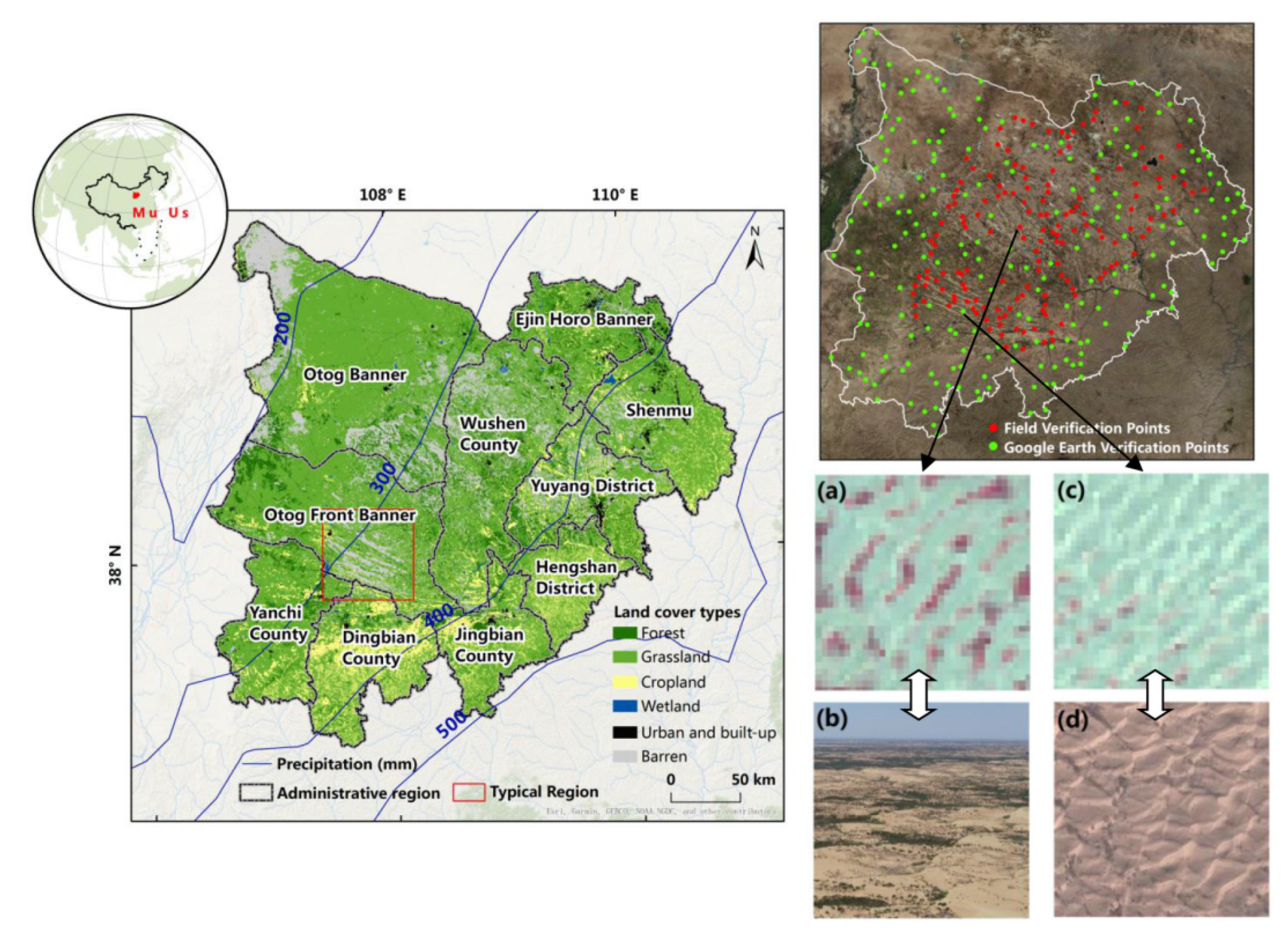
2.1. Study Area

The Mu Us Sandy Land is located between 106°26′–110°55′E and 36°48′–40°12′N, and includes 11 banners (counties, districts) in most areas of Ordos City in Inner Mongolia Autonomous Region, northern Yulin City in Shaanxi Province, and northeastern Ningxia Hui Autonomous Region, covering an area of approximately 87,353 km² (Figure 1). This area is located in the intermediate zone between the Ordos Plateau and the Loess Plateau and is a transitional zone between wind erosion and water erosion following from sandy to loess areas. The elevation ranges from 1000 to 1400 m, and the terrain slopes from northwest to southeast [29]. Mu Us Sandy Land has a semi-arid climate that transitions from temperate grassland to desert grassland and is the transition zone from animal husbandry to agriculture, which belongs to the typical temperate continental climate. The annual average precipitation is 150–500 mm, decreasing from southeast to northwest. The annual average temperature is 5.5–8.7 °C, the annual evapotranspiration is 2200–3000 mm, and the annual average wind speed is 2.00–3.60 m·s⁻¹ [29]. In the study area, both zonal and non-zonal soil coexist. The zonal soil consists primarily of chestnut soil, while the non-zonal soil consists primarily of aeolian sandy soil, swamp soil, saline-alkali soil, and meadow soil. The vegetation is primarily grassland and sandy shrub vegetation, with Artemisia ordosica as the dominant plant species [35]. Mu Us Sandy Land is one of China’s four major sand lands and a key component of the northern farming-pastoral ecotone. It is situated in a typical fragile ecological environment and is a significant source of sediment in the Yellow River. As a sensitive ecological transition zone in northern China, the Mu Us Sandy Land has always been an important region of desertification research [36].

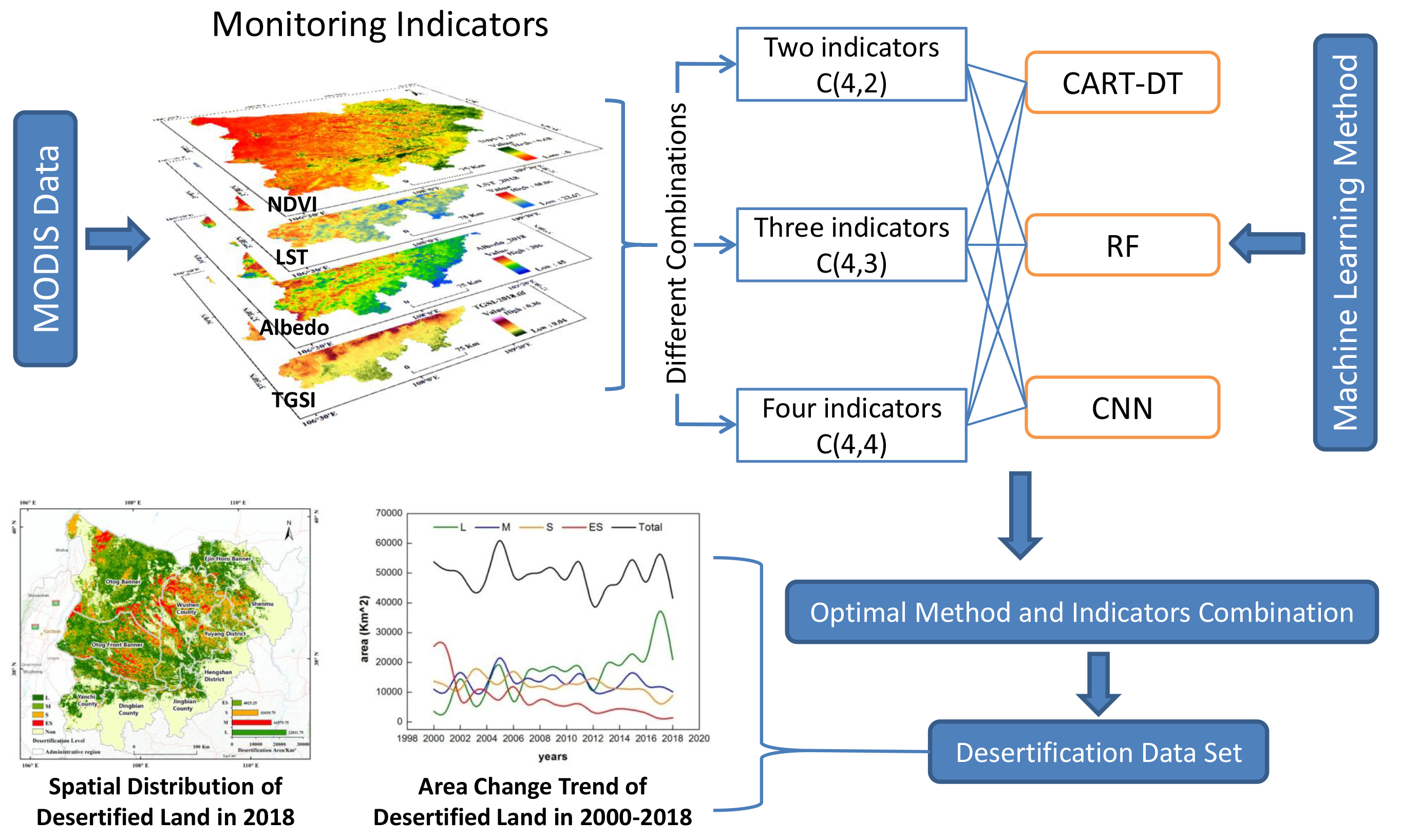
2.2. Data Source and Preprocessing

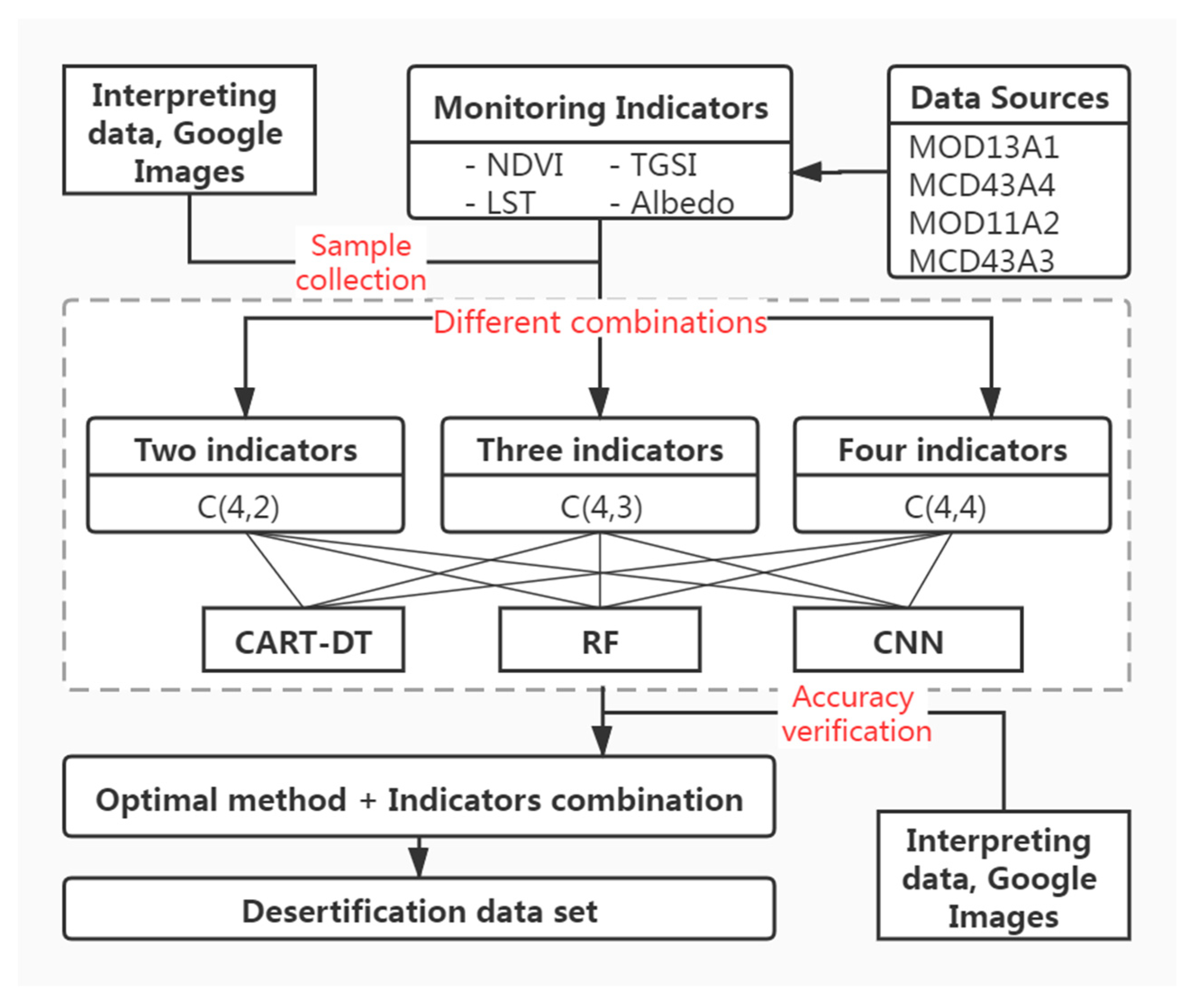
Remote sensing data—The Terra moderate-resolution imaging spectroradiometer (MODIS) product data provided by NASA LAADS DAAC data center (https://ladsweb.modaps.eosdis.nasa.gov/, 31 December 2018) were used as remote sensing inversion indexes for desertification monitoring in this study (

Table 1. Summary of the four typical surface parameters.

Product	Data Used	Spatial Resolution	Temporal Resolution	Reference
NDVI	MOD13A1	500 m	16 d	[37] Fan and Liu (2016)
Albedo	MCD43A3	500 m	Daily	[38] Wu et al. (2018)
LST	MOD11A2	1000 m	8 d	[39] Wan (2014)
TGSI	MCD43A4	500 m	Daily	[40] Liu et al. (2018)

Note: NDVI, Normal Difference Vegetation Index; LST, Land Surface Temperature; TGSI, Topsoil Grain Size Index. The source data (MODIS) of each index are avaliable during the growing season (May–October) of 2000 to 2018.

), including surface reflectance (MCD43A4), albedo (MCD43A3), vegetation index (MOD13A1), and land-surface temperature (MOD11A2). The study also employed USGS-shared Landsat8 OLI remote sensing images of 2015 (https://glovis.usgs.gov/, 31 October 2015) to visually interpret and generate a sample database of machine learning.

Vegetable Index data—Vegetation Indices 16-Day L3 Global 500 m product (MOD13A1) from 2000 to 2018 was used to acquire the normalized difference vegetation index (NDVI) in this study. The NDVI is derived from atmospherically corrected reflectance in the red, near-infrared, and blue wavebands [37,41,42], as shown in Equation (1):

$$NDVI=\frac{{\rho }_{nir }-{\rho }_{red }}{{\rho }_{nir }+{\rho }_{red }},$$

(1)

where ${\rho }_{nir }$, ${\rho }_{red}$ are the surface reflectance for the near-infrared and red bands.

Land surface temperature (LST) data—MOD11A2 land surface temperature product data are retrieved at 1 km pixels by the generalized split-window algorithm, with 1 km spatial resolution and 8-day temporal resolution, provided along with the daytime and nighttime surface temperature. This study used daytime LST data after denoising from 2000 to 2018, which were converted to Celsius temperature using the formula: LST (°C) = DN × 0.02 − 273.15 [39].

Albedo data—The Albedo Daily L3 Global 500 m product (MCD43A3) from 2000 to 2018 was used to derive the albedo in this study. The albedo of the product was calculated based on the Bidirectional Reflectance Distribution Function (BRDF) model after atmospheric correction [38]. These data included black space albedo and white space albedo of seven narrow bands and three wide bands (visible band 0.3–0.7 μm, near-infrared band 0.7–5.0 μm and shortwave band 0.3–5.0 μm). In this study, the white sky albedo in the shortwave band was selected.

Topsoil Grain Size Index (TGSI) data—The Topsoil Grain Size Index was calculated using the daily composite Albedo product (MCD43A4; [40,43]) from 2000 to 2018. Albedo measurements were derived simultaneously from the BRDF for bands 1–7.

$$TGSI=\frac{{\rho }_{red }-{\rho }_{blue }}{{\rho }_{red }+{\rho }_{blue}+{\rho }_{gree}},$$

(2)

where ${\rho }_{red }$, ${\rho }_{blue}$ and ${\rho }_{green }$ are the albedo measurements for the red, blue and green bands, respectively.

The above index data were chosen in this study combined with vegetation, soil and environmental information representative of desertification. All of these data were processed by mosaic, cutting and monthly value synthesis, and the monthly average of the vegetation growing season (May–October) was chosen as the model input data.

2.3. Methods

This section elaborates on different machine learning methods for desertification monitoring. The evaluation methods of result precision and field verification of training samples are also included to identify modeling processes, analysis and evaluation.

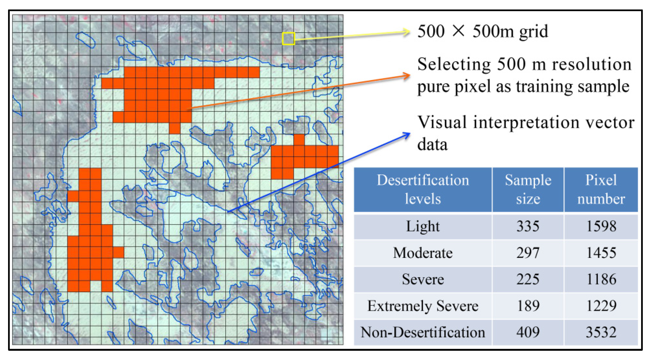
2.3.1. Classification System, Model Samples and Field Verification

Classification System of Desertification Land

The surface landscape characteristics of aeolian desertification land are primarily the appearance of surface wind and sand activities, which are characterized by an increasing proportion of mobile dunes, decreasing vegetation coverage and soil coarsening. According to the current remote sensing methods and the characteristics of surface morphology, vegetation and natural landscape of desertification land, this study divided desertification land into four levels: light, moderate, severe and extremely severe (

Table A1. Classification system of desertification land.

Levels of Desertification Land	Percentage of Mobile Sand Dunes (%)	Vegetation Cover (%)	Landscape Characteristics
Light	<5	50–70	Quicksand is speckled and appears on the windward slope of sand dunes. Vegetation begins to decline, but most of the area still resembles the original landscape.
Moderate	5–25	30–50	There are degenerate plants and low shrub sand piles.
Severe	25–50	10–30	Sand dunes are in a half-shifting state; a large number of sandy pioneers’ plants appear.
Extremely severe	>50	<10	Sand dunes are in a shifting state; vegetation disappears regionally.

, [11]). Using the spectral differences in remote sensing images of ground object types and the desertification land classification system, the interpretation marks of desertification land were established based on the texture, color, brightness, shape and other characteristics of remote sensing images of different desertification land (

Table A2. Interpretation signs and characteristics of desertification land.

Levels of Desertification Land	Tone and Texture of Landsat Image	Photo of Landscape	Landsat Image (Combination of NIR, RED, and GREEN Bands)
Light	Vegetation is light red and discontinuously distributed. Sparse sand covers the vegetation in spots with milky or yellow patches.
Moderate	Fixed and semi-fixed sand dunes are depicted as strips or plaques with red and white spots. Red vegetation accounts for 30–50% of the area.
Severe	Semi-fixed and semi-mobile sand dunes are patchy, with light yellow or yellow-white base colors and a few red spots.
Extremely severe	Mobile sand dunes are shown as scaly, with clear ripples, and the overall display is bright white or light yellow with few red spots.

, [29]).

The Sample Selection and Sample Size

Since the spatial resolution of the MODIS data to be classified was 500 m, the study established a 500 × 500 m grid, and selected the 500 m resolution of the pure pixel set as the training sample to refer to the visual interpretation results based on Landsat images. The sample size of different levels of desertification land is shown in Figure 2, and the total sample size reaches 1455 (9000 pixels, evenly distributed on different levels of desertification land) in machine learning methods.

Model Samples Verification

The study chose 400 verification points (including 191 field verification points and 209 Google image verification points, Figure 1) to validate and improve the sample database’s accuracy.

2.3.2. Models Used—CART-DT, RF and CNN

Classification and Regression Tree-Decision Tree (CART-DT)

The decision tree algorithm [44] is a fundamental classification method that is based on a tree structure and can be thought of as a set of if-then rules. It consists of one root node, several internal nodes, and several leaf nodes, with the leaf node representing the outcome of the decision. It is non-parametric and nonlinear because the model results are simple to explain [12]. The CART algorithm assumes that the decision tree is all binary trees, and the decision tree divides each feature recursively into two parts before obtaining the decision result. In other words, the feature space is divided into finite elements through continuous division, and the probability distribution of prediction is determined by these elements [45]. The idea behind constructing a CART-DT is to generate a large tree with multiple levels and leaf nodes based on the overall sample data, then delete it to generate a series of sub-trees, from which the appropriate size of the tree is selected to classify the data. It is further subdivided into tree growth and tree pruning. To prune the optimal tree, the CART algorithm employs the cross-validation method. In this study, the test error is evaluated using 10-fold cross validation. At the same time, the maximum depth of the decision tree model is 2, and there are at least 10 samples in the node data set to continue the division of the node data set to prevent overfitting or underfitting of the model and reduce the time complexity of the training model, and a leaf node must contain at least six samples, and the model can only contain four leaf nodes. This model was run using the package scikit-learn in Python version 2.7 software [46].

Random Forest (RF)

RF is a machine learning method that assigns a value or class to a response variable by using regression or classification trees. In the classification mode, RF uses an ensemble classification with multiple classifiers and a fully non-parametric statistical method [47]. There are hundreds of decision trees built into RF classification, and their decisions are usually combined by multiple votes. The general principle of group training is that ensemble models are superior to single models, avoiding the clashes between feature subsets [48]. Consequently, the RF classification is extensively used to process remote sensing imagery. The important training options in the RF model are the number of trees, the maximum number of features in RF splitting, and the variant for the sampling process [49]. Following the results of the experiments, the maximum number of trees used in this study was set to 100, and this study selected the square root of the total feature as the maximum number of features, which concerns the best splitting scenario. Additionally, the out-of-pocket (OOB) sample statistics are used in this model. When new input is used, the OOB sample statistics determine how the model will be implemented. This model was run using the package Random Forest in Python version 2.7 software [50].

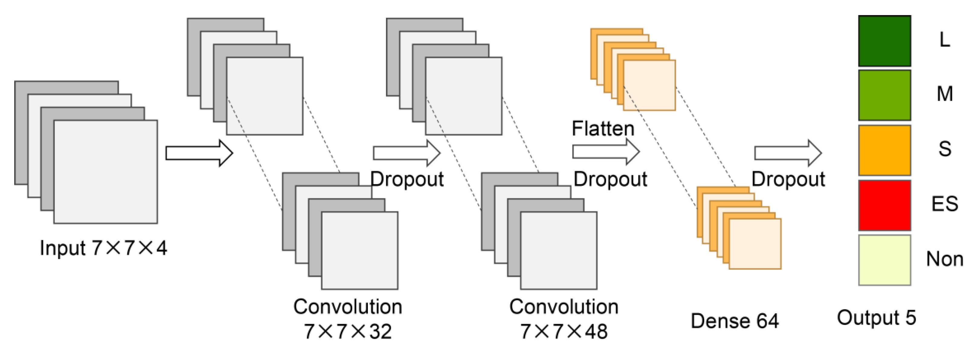
Convolutional Neural Networks (CNN)

CNN is a deep neural network originally designed for image analysis [51]. This model is analogous to the neurons in the brain and it is a normalized version of multi-layer perceptrons in fully interconnected networks [52]. Specifically, the CNN consists of a single input layer, several hidden layers and a layer of output. Convolutional layers, activation function, pooling layers and fully connected layers are structurally included in the hidden layers [53]. CNN requires much less preprocessing than other classification algorithms and produces better results as the number of training data increases [54].

The CNN structure of this study is shown in Figure 3. The input data of the input layer are the normalized sample grid, and the size of each sample is 7 × 7, with four bands (four monitoring indicators). In general, the higher the number of convolution layers, the more abstract features can be extracted. Because the pooling layer is usually more important in target detection, this model only has two convolution layers. The activation function ReLU can reduce the output of some neurons to zero, increasing the network’s sparse expression ability and preventing overfitting in this study. SoftMax, a classifier modeled by polynomial distribution and suitable for classifying multiple mutually exclusive categories, was used in the output layer. Dropout is used to prevent overfitting of the model training in order to improve the network’s generalization ability. Some neurons are randomly deleted during each iteration of the model training, avoiding the simultaneous updating of all feature weights at each iteration and, thus, weakening the synergistic effect between various features. Dropout was set to 0.25 in this model. This model was run using the package Tensorflow in Python version 2.7 software [55].

2.3.3. Models Accuracy Assessment

The confusion matrix approach is often used to evaluate land use/land cover(LU/LC) classification outcomes, it is a standard format accuracy of the evaluation, with k rows and k columns (

Table 2. The confusion matrix.

		Predicted Results
		L	M	S	ES	Non
Actual Results	L	p11	p12	p13	p14	p15
	M	p21	p22	p23	p24	p25
	S	p31	p32	p33	p34	p35
	ES	p41	p42	p34	p44	p45
	Non	p51	p52	p35	p45	p55
$p_{ij}$ is the proportion of sample size (in the i, jth cell) to total sample size.
$p_{i+}$ is the sum of rows i; $p_{+i}$ is the sum of columns i.
The accuracy of Class i prediction is true: $Precision=\frac{p_{ii}}{p_{+i}}$; The accuracy of Class i actual is true: $Recall=\frac{p_{ii}}{p_{i+}}$.
Prediction consistency (overall classification accuracy, OA): $P_o={\displaystyle \sum _{i=1}^k{p}_{ii}}$;
Actual consistency: $P_e={\displaystyle \sum _{i=1}^k{p}_{i+}{p}_{+i}}$, k = 5.
Kappa coefficient: $k=\frac{P_o-P_e}{1-P_e}$; Kappa coefficient of class i: $k_i=\frac{p_{ii}-p_{i+}{p}_{+i}}{p_{+i}-p_{i+}{p}_{+i}}$.

Note: L—light desertification, M—moderate desertification, S—severe desertification, ES—extremely severe desertification, Non—non-desertification.

); k = 5 is used to represent five different levels of desertification in the study. This method provides an assessment of the classified results and referenced data [56,57].

Precision and recall are used to evaluate each class prediction result. Prediction precision is the number of positive samples correctly classified all of the positive sample accounts for the number of divided classifier ratio; Recall (Sensitivity) is the number of positive samples correctly classified accounting for the proportion of the number of positive samples. The overall accuracy (OA) and Kappa coefficient resulting from the confusion matrix were used to evaluate model accuracy [58,59]. In this study, both of these measurement approaches were used to evaluate desertification classification results. Simultaneously, the variance analysis of Kappa of different classes was used to evaluate the significance of differences between groups of classification results.

2.3.4. Landscape Index and Surface Wetness Index

In this study, the landscape indices (fragmentation index and separation index) were used to analyze and evaluate the monitoring results of desertification; the fragmentation index refers to the fragmentation degree of landscape segmentation, reflecting the complexity of landscape spatial structure [60]. The formula is:

FN₁ = (N_p − 1)/N_c,

(3)

where FN₁ is the landscape fragmentation index of the whole study area; N_p is the total number of landscape patches; N_c is the ratio of the total area of the study area to the minimum patch area. FN₁ ∈ (0, 1), 0 means that the landscape is completely undamaged, and 1 means that the landscape is completely destroyed.

The separation index refers to the degree of dispersion (or agglomeration) of the spatial distribution of different patches in a landscape. The formula is:

N_i = D_i/S_i,

(4)

where N_i is the separation index of landscape type i; D_i is the distance index of landscape type i; $D_i=\frac{1}{2}\sqrt{\frac{n}{A}}$, n is the number of patches of landscape type i; A is the total area of the study area (km²); S_i is the area index of landscape type i, S_i = A_i/A, A_i is the area of landscape type i. The separation degree is used to analyze the spatial distribution characteristics of landscape elements. The larger the separation degree is, the more discrete the patches are and the greater the distance between patches is.

The surface wetness index (SWI) is commonly used to detect inter-annual dry/wet climate change [61]. Therefore, SWI was applied in this study to determine the occurrence time of extreme dry/wet climate in Mu Us Sandy Land from 2000 to 2018.

$$SWI=\frac{{{\displaystyle \sum }}_{i=1}^{12}{P}_i}{{{\displaystyle \sum }}_{i=1}^{12}P{E}_i},$$

(5)

where P_i and PE_i are monthly precipitation and potential evapotranspiration, respectively. SWI < 0.05 is extreme arid area, 0.05 ≤ SWI < 0.20 is arid area, 0.20 ≤ SWI < 0.50 is semi-arid area, 0.50 ≤ SWI < 0.65 is semi-humid arid area, SWI ≥ 0.65 is humid area.

Monthly precipitation and potential evapotranspiration data for 2000–2018 are derived from National Meteorological Information Center (http://data.cma.cn/, 31 December 2018).

2.3.5. Scheme Optimization

Given the uncertainty of selecting monitoring indicators and the different advantages of machine learning methods, we aim to explore the ideal combination of monitoring indicators and the optimal machine learning method suitable for the study area by excluding the repeated expression of monitoring information. We propose the following scheme (Figure 4).

3. Results

The accuracy of desertification information under different machine learning algorithms and index combinations was compared, and the optimal model and index combination of desertification land classification in the Mu Us Sandy Land was identified. The optimal model and index combination were then used to obtain the spatial distribution of desertified land in the Mu Us Sandy Land in 2018, and the temporal change of desertification areas in the study area from 2000 to 2018.

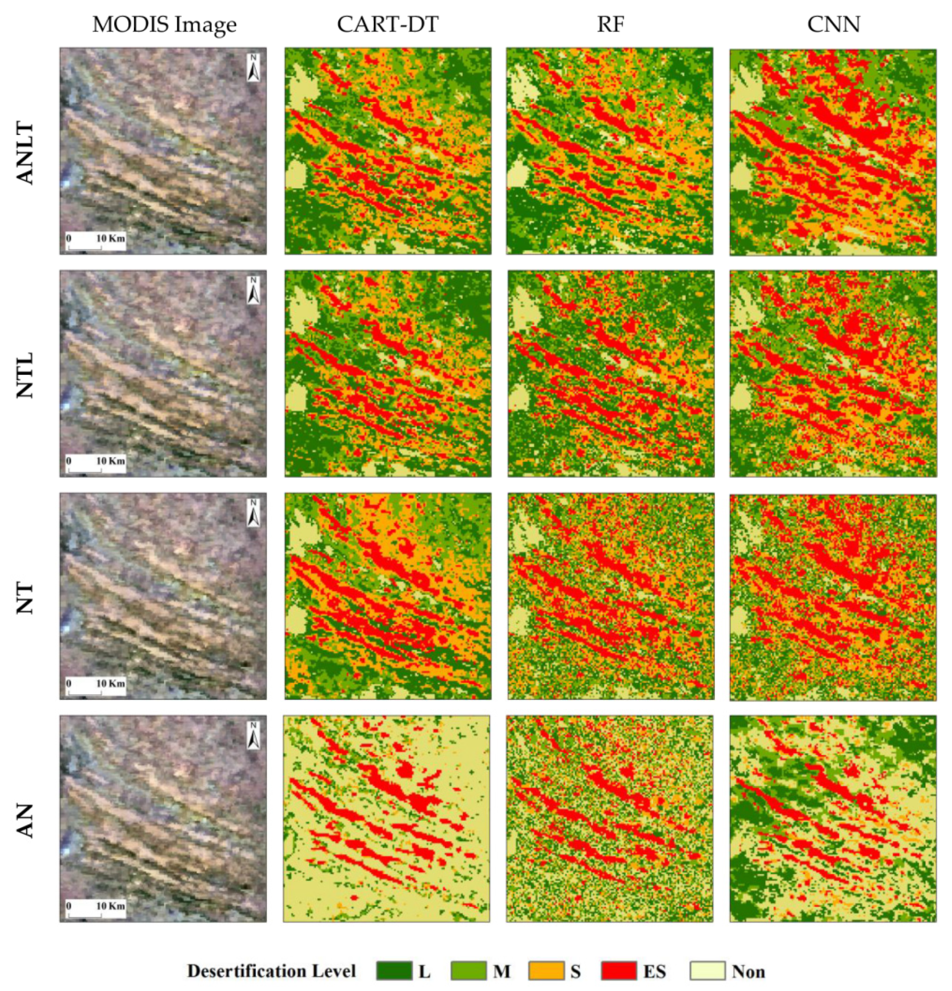
3.1. Comparison of Model Accuracy

Combined with vegetation information (NDVI), temperature information (LST), topsoil information (TGSI) and surface radiation information (Albedo), three machine learning methods of CART-DT, RF and CNN were applied to obtain 33 groups of desertification land classification based on the optimization scheme in Mu Us Sandy Land. Using the overall accuracy and Kappa coefficient and comparing 33 groups of accuracy results of extracting desertification information via machine learning algorithm, we found that the combination accuracy of the RF model and four indicators (ANLT) is the highest with an overall accuracy of classification of 87.67% and a Kappa coefficient of 0.84 (

Table 3. The results of model accuracy with different indicator combinations.

Different Combinations		CART-DT		RF		CNN
		OA(%)	Kappa	OA(%)	Kappa	OA(%)	Kappa
C(4,4)	ANLT	69.07	0.59	87.67	0.84	78.46	0.73
C(4,3)	ANL	60.05	0.45	82.86	0.77	72.08	0.68
	ANT	64.32	0.52	83.72	0.78	74.78	0.69
	ATL	66.61	0.55	85.25	0.80	76.29	0.71
	NTL	68.17	0.58	85.74	0.81	76.47	0.71
C(4,2)	AN	52.32	0.32	77.65	0.70	61.42	0.58
	AL	54.68	0.36	78.88	0.72	65.87	0.60
	AT	58.69	0.44	80.47	0.74	68.22	0.62
	NL	57.79	0.41	79.68	0.73	67.48	0.61
	NT	61.34	0.48	81.40	0.75	72.20	0.66
	TL	58.36	0.44	80.40	0.74	68.37	0.62

Note: Different Combinations are identified in the form of alphabetical combinations of indicators, in which A is Albedo; N is NDVI; L is LST; T is TGSI; OA is Overall accuracy; Kappa is Kappa coefficient. C(4,4): One combination of four indicators selected from four indicators; C(4,3): Four combinations of three indicators selected from four indicators; C(4,2): Six combinations of two indicators selected from four indicators.

). As shown in Table 3, from the perspective of the algorithm, the accuracy of the RF model is the highest, the CNN is the second-highest, and the CART-DT algorithm is the lowest. Considering the combination of indicators involved, the accuracy of desertification information extraction is from high to low: the combination of four indicators, the combination of three indicators, and the combination of two indicators.

Unexpectedly, the results also show that the combination of the two indicators with the highest accuracy is NT, and the combination of the corresponding three indicators is NTL. In particular, the lowest accuracy of the combination of two indicators is AN, and the lowest accuracy of the three indicators is ANL, which is even lower accuracy than the two indicators NT.

We now focus, firstly, on the nine groups of classification results with the highest accuracy under different index combinations and methods in the typical area, and, secondly, on the three groups of classification results of AN combinations with the lowest accuracy (Figure 5). The patch separation degree is low for classification results obtained by the CART-DT algorithm (

Table 4. The landscape indices of desertification land based on different combinations.

Combination		Fragmentation Index	Separation Index_ES
CART-DT	ANLT	0.078	1.47
	NTL	0.071	1.03
	NT	0.052	0.67
	AN	0.013	0.46
RF	ANLT	0.091	1.12
	NTL	0.105	1.55
	NT	0.376	1.74
	AN	0.411	1.68
CNN	ANLT	0.054	0.82
	NTL	0.086	1.13
	NT	0.235	1.55
	AN	0.022	0.66

), and the accuracy decreases in turn with the decrease in the index. Most categories of desertified land from the AN combination are identified as non-desertified land, except for extremely severe desertification. The classification results extracted by the RF algorithm showed significant patch fragmentation with decreasing index accuracy. This trend is especially apparent for the AN combination, except for extremely severely desertified land (Table 4). The classification result produced by the CNN algorithm also decreases with the reduction in the index accuracy, but the law of patch separation (fragmentation) is not obvious, and there is an overestimation of the area of extremely severely desertified land (Table 4).

3.2. Optimal Classification Results

This study obtained the classification accuracy of desertification in Mu Us Sandy Land in 2018 by applying the optimal RF model and ANLT combination of monitoring indices. As shown in

Table 5. Prediction accuracy of desertification at different levels based on random forest model.

Level of Desertification	Prediction Accuracy (%)
	Prediction Precision	Prediction Recall
Light Desertification (L)	80.43	81.57
Moderate Desertification (M)	82.05	82.96
Severe Desertification (S)	83.19	84.19
Extremely Severe Desertification (ES)	94.84	92.38
Non-Desertification (Non)	93.92	90.08
Overall Classification Accuracy	87.67

, the classification accuracy of light desertification is the lowest (precision = 80.43%, recall = 81.57%) and the classification accuracy of the extremely severe desertification is the highest (precision = 94.84%, recall = 92.38%). The results of the confusion matrix of accuracy show that the confusion pixels of light and moderate desertification account for a large proportion in the results of the automatic classification based on the machine learning algorithm and affect the prediction accuracy.

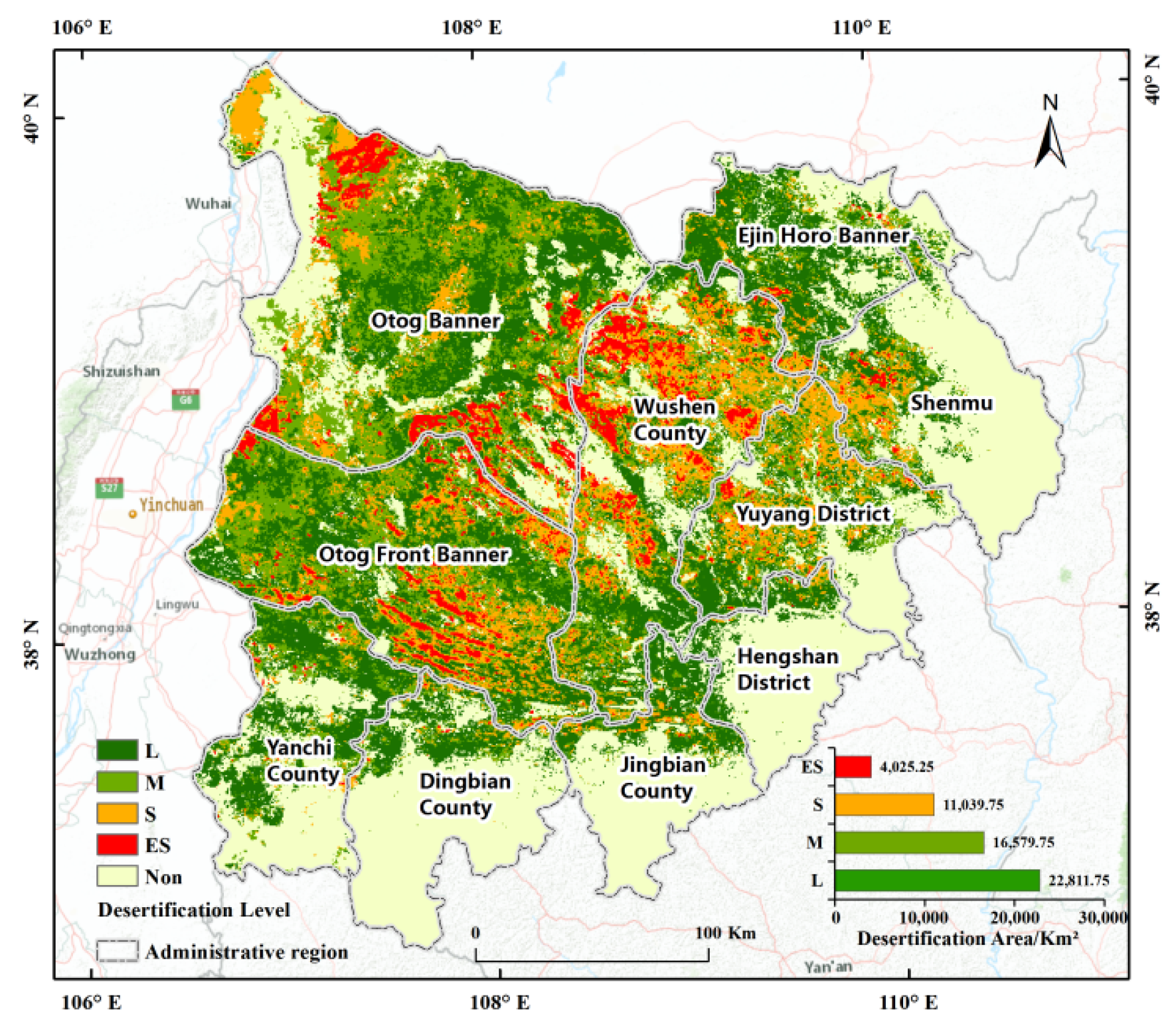
3.3. Distribution of Desertification in Mu Us Sandy Land

In the following sections, we discuss the spatial distribution of desertified land in Mu Us Sandy Land in 2018 and investigate the temporal changes to the area of desertified land from 2000 to 2018. The classification results of the optimal scheme are based on the RF algorithm and four monitoring indicators (ANLT).

3.3.1. Current Status and Spatial Distribution of Desertified Land in 2018

The results of the computer-automatic classification show that the desertified land has mainly experienced light desertification, accounting for 41.89% of the total desertified land area in Mu Us Sandy Land (Figure 6), followed by extremely severe and severe desertified land. The proportion of moderate desertified land is the lowest (7.39%). Desertified land is principally distributed in the hinterland and the northwest margin of the sandy land. The hinterland is mainly extremely severe and severe desertified land, while the northwest, west and north of the hinterland are generally light and severe desertified land. The southeast edge of sandy land is the transitional region from sandy land to loess area and is dominated by non-desertified land that is not at risk from desertification.

From the perspective of the administrative division, the desertified land is mainly distributed in Otog Banner and Otog Front Banner in the west of Mu Us Sandy Land and Wushen Banner in the middle of the sandy land (

Table 6. Area of desertification land in various counties at different levels in 2018.

Counties	L/km2	M/km2	S/km2	ES/km2	Total/km2	Percentage/%
Otog Banner	5431.85	6003.52	2538.33	1321.37	15,295.07	28.20
Otog Front Banner	4431.60	4036.53	2475.10	968.33	11,911.57	21.96
Wushen County	2709.19	2247.98	2905.14	1326.61	9188.92	16.94
Yuyang District	1568.00	1334.38	1412.71	136.23	4451.32	8.21
Ejin Horo Banner	2576.71	703.83	348.52	69.30	3698.35	6.82
Yanchi County	2294.00	907.84	246.83	52.62	3501.28	6.46
Shenmu	896.40	611.87	649.29	98.15	2255.71	4.16
Jingbian County	1132.03	213.22	193.31	16.88	1555.44	2.87
Dingbian County	999.63	327.64	166.93	19.68	1513.89	2.79
Hengshan District	680.02	104.55	72.19	6.28	863.04	1.59

Note: L—light desertification, M—moderate desertification, S—severe desertification, ES—extremely severe desertification.

), which together account for 67.10% of the total area of desertified land in the study area. Specifically, Otog Banner has the largest proportion of desertified land (28.20%) and contains all different levels of desertification. The area of desertified land in Wushen Banner accounts for 16.94%, ranking third out of the different administrative divisions, but contains the largest area of severely and extremely severely desertified land. The banners (counties/districts) with the least desertified land are Hengshan District, Dingbian County and Jingbian County in the south of the sandy land, where the proportion of desertified land is less than 3.00%.

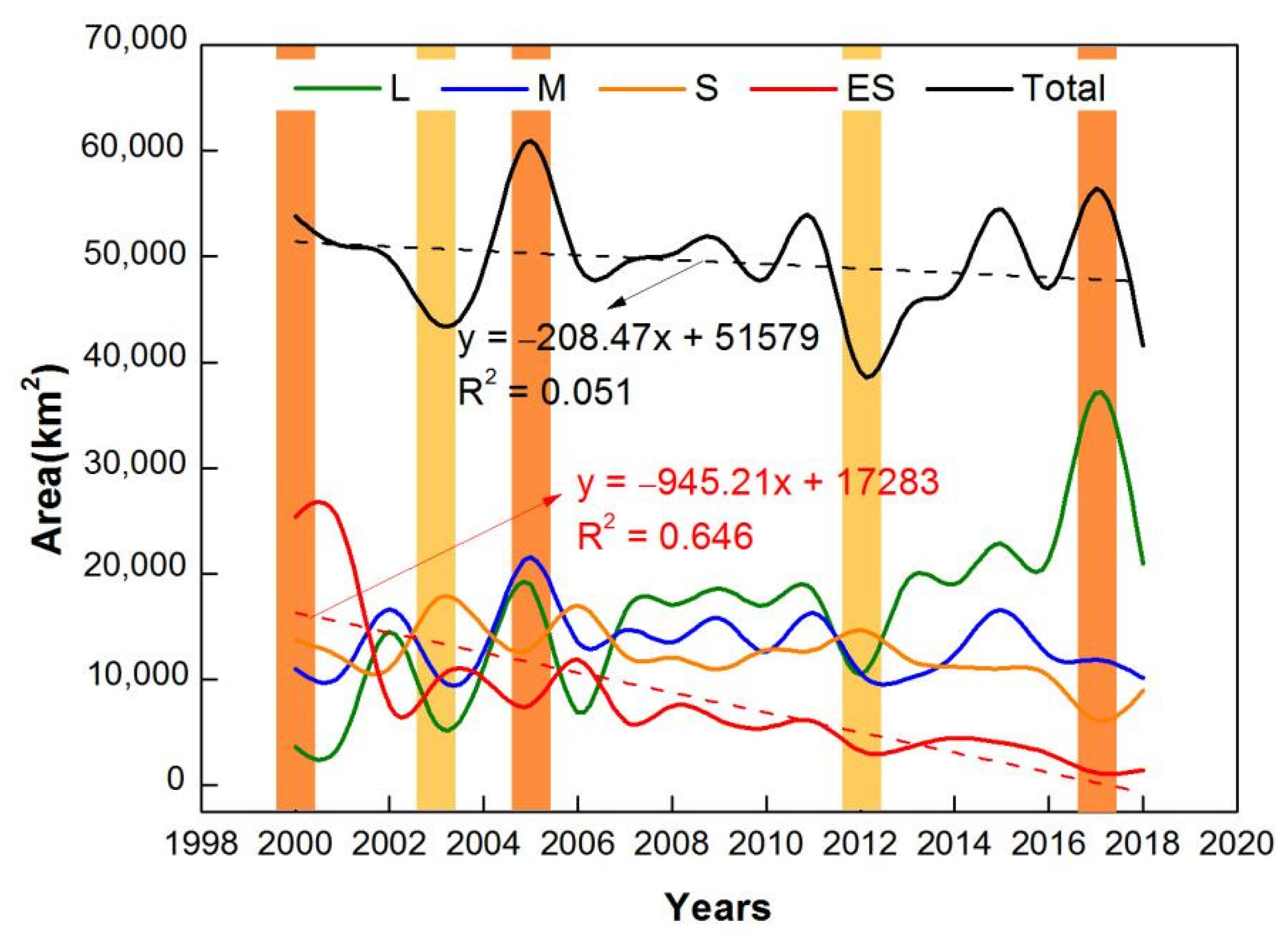
3.3.2. The Changes in Time Series Desertification Land from 2000 to 2018

Since the 1960s, climate warming caused by human activities and land use cover change (LUCC) has aggravated the problem of grassland degradation and desertification in northern China [10]. However, since 2000, desertification has been reduced across China by environmental initiatives [6]. The results of this study show that there is a decreasing trend of desertified land in Mu Us Sandy Land since 2000, especially for extremely severe desertified land. The area of moderate and severe desertified land has remained relatively stable over the past 18 years, and the area of light desertification has increased. Since 2007, the area of extremely severe desertified land was smaller than that of the other categories, and the area of light desertified land was greater than that of all other categories combined (Figure 7). The interannual changes in the area of light desertified land and total desertified land showed strong volatility, and the magnitude of fluctuation was relatively consistent (Figure 7 and Figure 8).

4. Discussion

4.1. The Optimal Method and Index Combination for Desertification Monitoring in Mu Us Sandy Land

The results of this study show that the random forest method outperforms all other models in the extraction of desertified land based on medium–low-resolution remote sensing images. This finding corresponds to previous studies on image classification whereby the RF classification accuracy is higher than the support vector machine and decision tree using medium–low-resolution data resources [62]. The CNN classification accuracy is lower than that of RF on a regional scale. As the CNN classification method is restricted to large-sized sample acquisitions [26], it is more suitable for global-scale classification research using the Google Earth Engine (GEE) platform to take advantage of the CNN classification benefit [63]. Fortunately, RF can solve the problem of over-fitting of decision tree and obtain high-precision classification results using the automatic acquisition of land cover data [64]. In the current era of big data, RF has become the most commonly used machine learning method for remote sensing image classification based on the GEE platform [63].

The combination of four indices (ANLT) obtains higher classification accuracy than that of two or three indices, irrespective of the method used to classify desertified land in the study area. Nonetheless, overall classification accuracy and Kappa comparability are poor across model groups. In the three groups, OA and Kappa were very close, with an overall accuracy of more than 85%. However, the variance analysis of Kappa coefficient k_i of ANLT and NTL (ANLT and NTL) classification results under the RF model showed that p = 0.006 (p = 0.005). This demonstrates that, while overall classification accuracy is similar, there are significant differences, and that the combination of RF and ANLT is the best classification scheme in the study. Notably, the contribution of each monitoring index varies greatly with threshold intervals for different levels of desertification (Figure 9). For example, we show that LST is the least important factor and does not separate the different levels of desertification. This finding indicates that the LST index is not effective for classifying desertified land, as corroborated by [12] in Horqin Sandy Land in northern China. In contrast, the TGSI index could directly separate non-desertified land from desertified land with excellent performance, which has also been shown for the Mongolian Plateau [19]. Albedo and NDVI are common remote sensing indicators that characterize vegetation and soil information to monitor desertification information. In our study region, these indices could effectively separate extremely severe desertified land (Figure 9), supporting the Albedo–NDVI point-to-point feature space model applied to study desertification in areas with high vegetation coverage [20]. However, these indices were not effective at distinguishing between light and moderate desertification (Figure 9), suggesting that additional indices should be considered.

4.2. The Spatio-Temporal Changes in Desertification in Mu Us Sandy Land Based on the Optimal Method and Index Combination

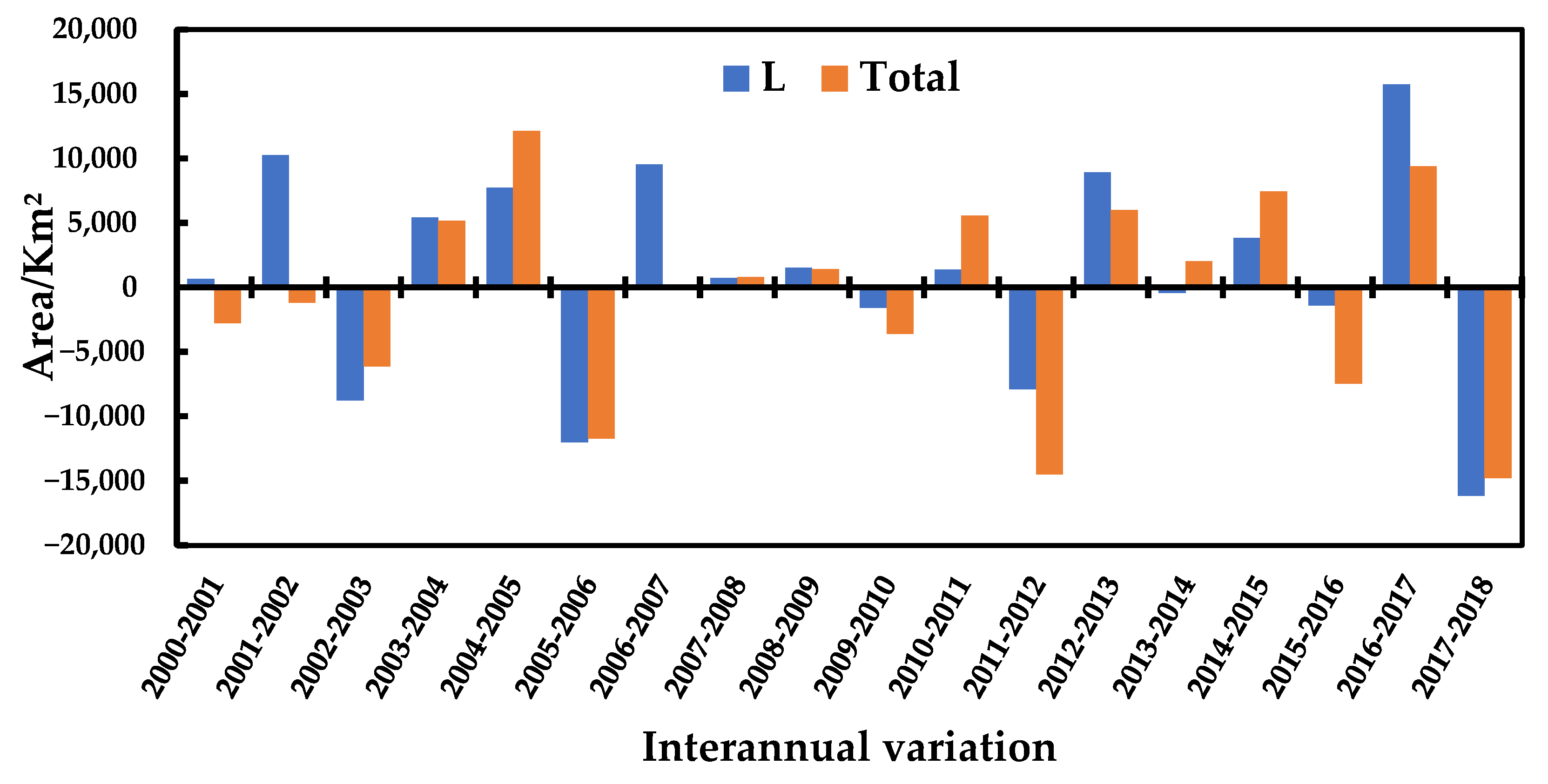
4.2.1. The Inter-Annual Volatility of Light Desertification Land Area

The results of this study demonstrate that the area of light desertified land fluctuates significantly between years (Figure 7), showing that it is difficult to quantify the area affected by light desertification. We believe this fluctuation is due to interannual variation in the monitoring indicators. As a result, we obtained the interannual variation trend of each monitoring index from 2000 to 2018 (Figure 10). The results revealed that all monitoring indices fluctuate across the time series. Zhang’s research indicated that the vulnerability of light desertified land to extreme climate change is unstable, meaning that these areas could be temporarily restored during periods with abundant rainfall or rapidly deteriorate into moderate desertified land during periods of drought [65]. Comparing the trend of the drought index SWI and the area of desertified land in Mu Us Sandy Land from 2000 to 2018 (Figure 7 and Figure 11), we find that both the light desertified land area and the total desertified land area fluctuated the most during extremely dry/wet years. In extremely dry years (2000, 2005 and 2017), the total desertified land area had three peaks, and in extremely wet years (2003 and 2012), the total desertified land area ushered in two valleys. The large fluctuation of the total desertified land area is primarily affected by the area of light desertification, which in turn responds to the occurrence of extreme climate events. Therefore, the volatility of light desertification could be defined as an unstable desertification area and represents an unavoidable problem in desertification monitoring. Future research should focus on how to determine the size and characteristics of this unstable region and how to protect against worsening desertification in the future.

4.2.2. The Transformation of Extremely Severe Desertification Land Area

As shown in Figure 7, the area of extremely severe desertification land in Mu Us Sandy Land has decreased since 2000, compared to all other land with different levels of desertification. Wang Tao et al. demonstrated that the change in desertification over time, being the pattern of change between the levels of desertification from “desertification to non-desertification”, requires a long process [6]. However, since 2000, there has been no obvious decrease in the total area of desertified land in Mu Us Sandy Land, indicating that the conversion of extremely severe desertified land to other desertified land is relatively active, and the desertification problem generally exhibits a reverse trend, primarily manifested as a decrease in the level of desertification. Then, according to this dynamic mechanism of desertification, the primary task of desertification control is the governance of extremely severe desertification.

4.2.3. The Ecological Restoration of Sandy Land

Combined with the changing trend of desertified land area and monitoring indicators in Mu Us Sandy Land from 2000 to 2018 (Figure 7 and Figure 10). After 2000, under the background of a warm and humid climate, Mu Us Sandy Land has experienced a series of ecological restoration projects and measures (i.e., the Return Grazing to Grass Program [66] and the “Three-North-Shelterbelt” Project [10]). Desertification has gradually been reduced, and the environment has been restored by the decrease in albedo and land surface temperature, the reduction in soil grain size and the increase in land surface greenness. This reduction in the area of desertified land in the Mu Us Sandy Land demonstrates that ecological restoration is an effective method to control desertification.

4.3. The Advantages and Limitations

According to MODIS data products, computer automatic classification technology is used to obtain high temporal resolution desertification data set in Mu Us Sandy Land. The results in this study provide useful mechanistic insights into the monitoring of desertification. The multi-index multi-model reveals the optimal method of desertification monitoring in the study area and is more advanced than using the single-index single model and multi-index single model. We also reveal that in the arid and semi-arid desert steppe areas of northern China, the area of light desertified land fluctuates significantly on interannual time scales depending on the weather and rainfall during a specific year. These fluctuations affect the total area of desertified land and could cause discrepancies in desertification monitoring results between different studies in the same region if not accounted for. Future research should quantify the potential area that is vulnerable to desertification to obtain more accurate results. The accuracy of the optimal monitoring scheme for the Mu Us Sandy Land should also be investigated for other regions.

5. Conclusions

In this study, the spatio-temporal patterns of desertification in the Mu Us Sandy Land were monitored with a machine learning model and multi-index remote sensing data. Since 2000, the total area of desertified land has reduced in the study region, although with significant interannual fluctuation primarily driven by changes in the area of light desertified land. The Random forest (RF) model is the optimal method for monitoring desertification in Mu Us Sandy Land using medium–low-resolution remote sensing images. The accuracy of land classification results extracted by the combination of four monitoring indicators (Albedo, NDVI, LST and TGSI) was the highest. Using the RF method and four monitoring indicators, the level of desertification in Mu Us Sandy Land was classified with an accuracy of 87.67%. However, the strong correlation between monitoring indicators may affect the classification accuracy due to the greater the information redundancy. The TGSI, which characterizes soil information, is an excellent monitoring index, while LST is not effective for classifying desertified land. The interannual variation in each index has a specific response to extreme climate, which may be the cause of the low classification accuracy of light desertification.

References

1. Ma, H.; Zhao, H. United Nations: Convention to combat desertification in those countries experiencing serious drought and/or desertification, particularly in Africa. Int. Legal Mater. 1994, 33, 1328–1382. [Google Scholar]
2. UNEP. Status of Desertification and Implementation of the United Nations Plan of Action to Combat Desertification: United Nations Environmental Program; UNEP: Nairobi, Kenya, 1992. [Google Scholar]
3. Hellden, U.; Tottrup, C. Regional desertification: A global synthesis. Global Planet. Change 2008, 64, 169–176. [Google Scholar]
4. Xu, D.; Zhang, X. Multi-scenario simulation of desertification in North China for 2030. Land Degrad. Dev. 2021, 32, 1060–1074. [Google Scholar] [CrossRef]
5. Chasek, P.; Akhtar-Schuster, M.; Orr, B.J.; Luise, A.; Ratsimba, H.R.; Safriel, U. Land degradation neutrality: The science-policy interface from the UNCCD to national implementation. Environ. Sci. Policy 2019, 92, 182–190. [Google Scholar] [CrossRef]
6. Wang, T.; Xue, X.; Zhou, L.; Guo, J. Combating aeolian desertification in northern China. Land Degrad. Dev. 2015, 26, 118–132. [Google Scholar] [CrossRef]
7. Kéfi, S.; Rietkerk, M.; Alados, C.L.; Pueyo, Y.; Papanastasis, V.P.; ElAich, A.; de Ruiter, P.C. Spatial vegetation patterns and imminent desertification in Mediterranean arid ecosystems. Nature 2007, 449, 213–217. [Google Scholar] [CrossRef]
8. Hanson, P.R.; Joeckel, R.M.; Young, A.R.; Horn, J. Late Holocene dune activity in the Eastern Platte River Valley, Nebraska. Geomorphology 2009, 103, 555–561. [Google Scholar] [CrossRef]
9. Du, H.; Zuo, X.; Li, S.; Wang, T.; Xue, X. Wind erosion changes induced by different grazing intensities in the desert steppe, Northern China. Agric. Ecosyst. Environ. 2019, 274, 1–13. [Google Scholar] [CrossRef]
10. Qi, Y.; Chang, Q.; Jia, K.; Liu, M.; Liu, J.; Chen, T. Temporal-spatial variability of desertification in an agro-pastoral transitional zone of northern Shaanxi Province, China. Catena 2012, 88, 37–45. [Google Scholar] [CrossRef]
11. Na, R.; Du, H.; Na, L.; Shan, Y.; He, H.S.; Wu, Z.; Zong, S.; Yang, Y.; Huang, L. Spatiotemporal changes in the Aeolian desertification of Hulunbuir Grassland and its driving factors in China during 1980–2015. Catena 2019, 182, 104123. [Google Scholar] [CrossRef]
12. Duan, H.; Wang, T.; Xue, X.; Yan, C. Dynamic monitoring of aeolian desertification based on multiple indicators in Horqin Sandy Land, China. Sci. Total Environ. 2019, 650, 2374–2388. [Google Scholar] [CrossRef]
13. Zhang, C.; Li, Q.; Shen, Y.; Zhou, N.; Wang, X.; Li, J.; Jia, W. Monitoring of aeolian desertification on the Qinghai-Tibet Plateau from the 1970s to 2015 using Landsat images. Sci. Total Environ. 2018, 619, 1648–1659. [Google Scholar] [CrossRef] [PubMed]
14. Xu, D.; Li, C.; Song, X.; Ren, H. The dynamics of desertification in the farming-pastoral region of North China over the past 10 years and their relationship to climate change and human activity. Catena 2014, 123, 11–22. [Google Scholar] [CrossRef]
15. Sternberg, T.; Tsolmon, R.; Middleton, N.; Thomas, D. Tracking desertification on the Mongolian steppe through NDVI and field-survey data. Int. J. Digit. Earth 2011, 4, 50–64. [Google Scholar] [CrossRef]
16. Tomasella, J.; Silva Pinto Vieira, R.M.; Barbosa, A.A.; Rodriguez, D.A.; Santana, M.D.O.; Sestini, M.F. Desertification trends in the Northeast of Brazil over the period 2000–2016. Int. J. Appl. Earth Obs. 2018, 73, 197–206. [Google Scholar] [CrossRef]
17. Sun, J.; Hou, G.; Liu, M.; Fu, G.; Zhan, T.; Zhou, H.; Tsunekawa, A.; Haregeweyn, N. Effects of climatic and grazing changes on desertification of alpine grasslands, Northern Tibet. Ecol. Indic. 2019, 107, 105647. [Google Scholar] [CrossRef]
18. Kempf, M. Monitoring landcover change and desertification processes in northern China and Mongolia using historical written sources and vegetation indices. Clim. Past Discuss. 2021, 2021, 1–29. [Google Scholar]
19. Wei, H.; Wang, J.; Cheng, K.; Li, G.; Ochir, A.; Davaasuren, D.; Chonokhuu, S. Desertification Information Extraction Based on Feature Space Combinations on the Mongolian Plateau. Remote Sens. 2018, 10, 1614. [Google Scholar] [CrossRef] [Green Version]
20. Guo, B.; Zang, W.; Han, B.; Yang, F.; Luo, W.; He, T.; Fan, Y.; Yang, X.; Chen, S. Dynamic monitoring of desertification in Naiman Banner based on feature space models with typical surface parameters derived from LANDSAT images. Land Degrad. Dev. 2020, 31, 1573–1592. [Google Scholar] [CrossRef]
21. Munkhnasan, L.; Woo-Kyun, L.; Seong, J.; Jong-Yeol, L.; Song, C.; Dongfan, P.; Chul, L.; Akhmadi, K.; Itgelt, N. Correlation between Desertification and Environmental Variables Using Remote Sensing Techniques in Hogno Khaan, Mongolia. Sustainability 2017, 9, 581. [Google Scholar]
22. Xu, D.; Kang, X.; Qiu, D.; Zhuang, D.; Pan, J. Quantitative Assessment of Desertification Using Landsat Data on a Regional Scale—A Case Study in the Ordos Plateau, China. Sensors 2009, 9, 1738–1753. [Google Scholar] [CrossRef] [PubMed] [Green Version]
23. Yue, Y.; Li, M.; Wang, L.; Zhu, A.-X. A data-mining-based approach for aeolian desertification susceptibility assessment: A case-study from Northern China. Land Degrad. Dev. 2019, 30, 1968–1983. [Google Scholar] [CrossRef]
24. Fan, Z.; Li, S.; Fang, H. Explicitly Identifying the Desertification Change in CMREC Area Based on Multisource Remote Data. Remote Sens. 2020, 12, 3170. [Google Scholar] [CrossRef]
25. Meng, X.; Gao, X.; Li, S.; Li, S.; Lei, J. Monitoring desertification in Mongolia based on Landsat images and Google Earth Engine from 1990 to 2020. Ecol. Indic. 2021, 129, 107908. [Google Scholar] [CrossRef]
26. Welsink, A. Comparing Classification of Ghana’s Complex Agroforestry Land Cover by a Random Forest and a Convolutional Neural Network with a Small Training Set. Master’s Thesis, Wageningen University, Wageningen, The Netherlands, 2020. [Google Scholar]
27. Pi, W.; Du, J.; Liu, H.; Zhu, X. Desertification Glassland Classification and Three-Dimensional Convolution Neural Network Model for Identifying Desert Grassland Landforms with Unmanned Aerial Vehicle Hyperspectral Remote Sensing Images. J. Appl. Spectrosc. 2020, 87, 309–318. [Google Scholar] [CrossRef]
28. Pi, W.; Du, J.; Bi, Y.; Gao, X.; Zhu, X. 3D-CNN based UAV hyperspectral imagery for grassland degradation indicator ground object classification research. Ecol. Inform. 2021, 62, 101278. [Google Scholar] [CrossRef]
29. Feng, K.; Wang, T.; Liu, S.; Yan, C.; Kang, W.; Chen, X.; Guo, Z. Path analysis model to identify and analyse the causes of aeolian desertification in Mu Us Sandy Land, China. Ecol. Indic. 2021, 124, 107386. [Google Scholar] [CrossRef]
30. Wu, B.; Ci, L.J. Developing stages and causes of desertification in the Mu Us sandland. Chin. Sci. Bull. 1999, 44, 845–849. [Google Scholar] [CrossRef]
31. Zhou, W.; Gang, C.; Zhou, F.; Li, J.; Dong, X.; Zhao, C. Quantitative assessment of the individual contribution of climate and human factors to desertification in northwest China using net primary productivity as an indicator. Ecol. Indic. 2015, 48, 560–569. [Google Scholar] [CrossRef]
32. Huang, L.; Xiao, T.; Zhao, Z.; Sun, C.; Liu, J.; Shao, Q.; Fan, J.; Wang, J. Effects of grassland restoration programs on ecosystems in arid and semiarid China. J. Environ. Manag. 2013, 117, 268–275. [Google Scholar] [CrossRef]
33. Guo, Q.; Fu, B.; Shi, P.; Cudahy, T.; Zhang, J.; Xu, H. Satellite monitoring the spatial-temporal dynamics of desertification in response to climate change and human activities across the Ordos Plateau, China. Remote Sens. 2017, 9, 525. [Google Scholar] [CrossRef] [Green Version]
34. Li, Y.; Cao, Z.; Long, H.; Liu, Y.; Li, W. Dynamic analysis of ecological environment combined with land cover and NDVI changes and implications for sustainable urban–rural development: The case of Mu Us Sandy Land, China. Clean. Prod. 2017, 142, 697–715. [Google Scholar] [CrossRef]
35. FAO; FAO/IUSS Working Group WRB. World Reference Base for Soil Resources 2006; World Soil Resources Reports; FAO: Rome, Italy, 2006; 103p. [Google Scholar]
36. Zhang, M.; Wu, X. The rebound effects of recent vegetation restoration projects in Mu Us Sandy land of China. Ecol. Indic. 2020, 113, 106228. [Google Scholar] [CrossRef]
37. Fan, X.; Liu, Y. A global study of NDVI difference among moderate-resolution satellite sensors. ISPRS J. Photogramm. 2016, 121, 177–191. [Google Scholar] [CrossRef]
38. Wu, X.; Wen, J.; Xiao, Q.; You, D.; Dou, B.; Lin, X.; Hueni, A. Accuracy Assessment on MODIS (V006), GLASS and MuSyQ Land-Surface Albedo Products: A Case Study in the Heihe River Basin, China. Remote Sens. 2018, 10, 2045. [Google Scholar] [CrossRef] [Green Version]
39. Wan, Z. New refinements and validation of the collection-6 MODIS land-surface temperature/emissivity product. Remote Sens. Environ. 2014, 140, 36–45. [Google Scholar] [CrossRef]
40. Liu, Q.; Liu, G.; Huang, C. Monitoring desertification processes in Mongolian Plateau using MODIS tasseled cap transformation and TGSI time series. J. Arid Land. 2018, 10, 12–26. [Google Scholar] [CrossRef] [Green Version]
41. Liang, D.; Cowles, M.K.; Linderman, M. Bayesian MODIS NDVI back-prediction by intersensor calibration with AVHRR. Remote Sens. Environ. 2016, 186, 393–404. [Google Scholar] [CrossRef]
42. Lin, X.; Niu, J.; Berndtsson, R.; Yu, X.; Zhang, L.; Chen, X. NDVI Dynamics and Its Response to Climate Change and Reforestation in Northern China. Remote Sens. 2020, 12, 4138. [Google Scholar] [CrossRef]
43. Xiao, J.; Shen, Y.; Tateishi, R.; Bayaer, W. Development of topsoil grain size index for monitoring desertification in arid land using remote sensing. Int. J. Remote Sens. 2006, 27, 2411–2422. [Google Scholar] [CrossRef]
44. Quinlan, J.R. Induction of decision trees. Mach. Learn. 1986, 1, 81–106. [Google Scholar] [CrossRef] [Green Version]
45. Larose, D.T.; Larose, C.D. Discovering Knowledge in Data: AnIntroduction to Data Mining; John Wiley & Sons: Hoboken, NJ, USA, 2014. [Google Scholar]
46. Lamrini, B. Contribution to Decision Tree Induction with Python: A Review. In Data Mining-Methods, Applications and Systems; IntechOpen: London, UK, 2020. [Google Scholar]
47. Breiman, L. Random forests. Mach. Learn 2001, 45, 5–32. [Google Scholar] [CrossRef] [Green Version]
48. Chan, J.C.; Paelinckx, D. Evaluation of Random Forest and Adaboost tree-based ensemble classification and spectral band selection for ecotope mapping using airborne hyperspectral imagery. Remote Sens. Environ. 2008, 112, 2999–3011. [Google Scholar] [CrossRef]
49. Belgiu, M.; Dragut, L. Random forest in remote sensing: A review of applications and future directions. ISPRS J. Photogramm. 2016, 114, 24–31. [Google Scholar] [CrossRef]
50. Chen, X.; Wang, T.; Liu, S.; Peng, F.; Tsunekawa, A.; Kang, W.; Guo, Z.; Feng, K. A New Application of Random Forest Algorithm to Estimate Coverage of Moss-Dominated Biological Soil Crusts in Semi-Arid Mu Us Sandy Land, China. Remote Sens. 2019, 11, 1286. [Google Scholar] [CrossRef] [Green Version]
51. Valueva, M.V.; Nagornov, N.N.; Lyakhov, P.A.; Valuev, G.V.; Chervyakov, N.I. Application of the residue number system to reduce hardware costs of the convolutional neural network implementation. Math. Comput. Simulat. 2020, 177, 232–243. [Google Scholar] [CrossRef]
52. Sarigul, M.; Ozyildirim, B.M.; Avci, M. Differential convolutional neural network. Neural Netw. 2019, 116, 279–287. [Google Scholar] [CrossRef]
53. Albawi, S.; Mohammed, T.A.; Al-Zawi, S. Understanding of a Convolutional Neural Network. In Proceedings of the International Conference on Engineering and Technology, Antalya, Turkey, 21–23 August 2017. [Google Scholar]
54. Yamashita, R.; Nishio, M.; Do, R.K.G.; Togashi, K. Convolutional neural networks: An overview and application in radiology. Insights Imaging 2018, 9, 611–629. [Google Scholar] [CrossRef] [Green Version]
55. Guirado, E.; Alcaraz-Segura, D.; Cabello, J.; Puertas-Ruiz, S.; Herrera, F.; Tabik, S. Tree Cover Estimation in Global Drylands from Space Using Deep Learning. Remote Sens. 2020, 12, 343. [Google Scholar] [CrossRef] [Green Version]
56. Lin, Y.; Liu, B.; Lu, Y.; Xie, F. Correlating Analysis on Spatio-temporal Variation of LUCC and Water Resources Based on Remote Sensing Data. In Proceedings of the 18th National Symposium on Remote Sensing of China, Wuhan, China, 20–23 September 2014; Tong, Q., Shan, J., Zhu, B., Eds.; SPIE: Bellingham, WA, USA, 2014; Volume 9158. [Google Scholar]
57. Fang, S.F.; Gertner, G.; Wang, G.X.; Anderson, A. The impact of misclassification in land use maps in the prediction of landscape dynamics. Landscape Ecol. 2006, 21, 233–242. [Google Scholar] [CrossRef]
58. Chen, Y.; Dou, P.; Yang, X. Improving Land Use/Cover Classification with a Multiple Classifier System Using AdaBoost Integration Technique. Remote Sens. 2017, 9, 1055. [Google Scholar] [CrossRef] [Green Version]
59. Ge, G.; Shi, Z.; Zhu, Y.; Yang, X.; Hao, Y. Land use/cover classification in an arid desert-oasis mosaic landscape of China using remote sensed imagery: Performance assessment of four machine learning algorithms. Glob. Ecol. Conserv. 2020, 22, e00971. [Google Scholar] [CrossRef]
60. Sui, D.Z.; Zeng, H. Modeling the dynamics of landscape structure in Asia’s emerging desakota regions: A case study in Shenzhen. Urban Plan. 2001, 53, 37–52. [Google Scholar] [CrossRef]
61. Zhuguo, M.A.; Dan, L.; Yuewen, H.U. The extreme dry/wet events in northern China during recent 100 years. J. Geogr. Sci. 2004, 14, 275–281. [Google Scholar] [CrossRef]
62. Sheykhmousa, M.; Mahdianpari, M.; Ghanbari, H.; Mohammadimanesh, F.; Ghamisi, P.; Homayouni, S. Support Vector Machine Versus Random Forest for Remote Sensing Image Classification: A Meta-Analysis and Systematic Review. IEEE J. Sel. Top. Appl. Earth Obs. Remote Sens. 2020, 13, 6308–6325. [Google Scholar] [CrossRef]
63. Tamiminia, H.; Salehi, B.; Mahdianpari, M.; Quackenbush, L.; Adeli, S.; Brisco, B. Google Earth Engine for geo-big data applications: A meta-analysis and systematic review. ISPRS J. Photogramm. 2020, 164, 152–170. [Google Scholar] [CrossRef]
64. Ma, L.; Li, M.; Ma, X.; Cheng, L.; Du, P.; Liu, Y. A review of supervised object-based land-cover image classification. ISPRS J. Photogramm. 2017, 130, 277–293. [Google Scholar] [CrossRef]
65. Zhang, G.; Biradar, C.M.; Xiao, X.; Dong, J.; Zhou, Y.; Qin, Y.; Zhang, Y.; Liu, F.; Ding, M.; Thomas, R.J. Exacerbated grassland degradation and desertification in Central Asia during 2000–2014. Ecol. Appl. 2018, 28, 442–456. [Google Scholar] [CrossRef] [Green Version]
66. Liang, P.; Yang, X. Landscape spatial patterns in the Maowusu (Mu Us) Sandy Land, northern China and their impact factors. Catena 2016, 145, 321–333. [Google Scholar] [CrossRef]
Figure 1. Study area. The information on precipitation, land cover, administrative division and verification points are shown. The 400 verification points include 191 field verification points and 209 Google Earth verification points. Field working time: 2015-07 to 2015-08: (a) Landsat OLI false-color synthesis image (S); (b) Field landscape photo (S); (c) Landsat OLI false-color synthesis image (ES); (d) Google Earth image (ES). S—severe desertification, ES—extremely severe desertification.
Remotesensing 14 02663 g001
Figure 2. The sample selection and sample size in the study.
Remotesensing 14 02663 g002
Figure 3. The convolutional neural network structure of this study. L—light desertification, M—moderate desertification, S—severe desertification, ES—extremely severe desertification, Non—non-desertification.
Remotesensing 14 02663 g003
Figure 4. Flow chart illustrating the data sources and methodology used in this study. CART-DT, RF, and CNN are different machine learning methods. MOD13A1, MCD43A4, MOD11A2 and MCD43A4 are different MODIS datasets.
Remotesensing 14 02663 g004
Figure 5. The desertification land classification results of the typical region based on different indicators and different machine learning methods with corresponding satellite images (see Figure 1 for the location of the typical region). L—light desertification, M—moderate desertification, S—severe desertification, ES—extremely severe desertification, Non—non-desertification.
Remotesensing 14 02663 g005
Figure 6. The spatial distribution of different levels of desertification in Mu Us Sandy Land in 2018. L-light desertification, M—moderate desertification, S—severe desertification, ES—extremely severe desertification, Non—non-desertification.
Remotesensing 14 02663 g006
Figure 7. The temporal trends of different levels of desertification in Mu Us Sandy Land from 2000 to 2018. L—light desertification, M—moderate desertification, S—severe desertification, ES—extremely severe desertification, Total—total desertification. 2000, 2005 and 2017 are classified as relatively arid years (orange histogram); 2003 and 2012 are classified as relatively humid years (yellow histogram).
Remotesensing 14 02663 g007
Figure 8. Interannual variability of the area of light desertification and total desertification in Mu Us Sandy Land from 2000 to 2018. L—light desertification, Total—total desertification.
Remotesensing 14 02663 g008
Figure 9. Threshold interval of monitoring indicators across different levels of desertification. In this study, 6000 pixels of monitoring indicators were randomly selected for box chart statistics from different desertified land. L—light desertification, M—moderate desertification, S—severe desertification, ES—extremely severe desertification, Non—non-desertification.
Remotesensing 14 02663 g009
Figure 10. The annual trends of desertification land monitoring indicators in Mu Us Sandy Land from 2000 to 2018.
Remotesensing 14 02663 g010
Figure 11. The temporal trends of SWI in Mu Us Sandy Land from 2000 to 2018. 2000, 2005 and 2017 (orange histogram) are defined as relatively arid years; 2003 and 2012 are defined as relatively humid years (yellow histogram).
Remotesensing 14 02663 g011