Article

A Spatial Long-Term Trend Analysis of Estimated Chlorophyll-a Concentrations in Utah Lake Using Earth Observation Data

by
Kaylee Brook Tanner
,
Anna Catherine Cardall
and
Gustavious Paul Williams
*
Department of Civil and Construction Engineering, Brigham Young University, Provo, UT 84602, USA
*
Author to whom correspondence should be addressed.
Remote Sens. 2022, 14(15), 3664; https://doi.org/10.3390/rs14153664
Submission received: 7 July 2022 / Revised: 27 July 2022 / Accepted: 29 July 2022 / Published: 30 July 2022
(This article belongs to the Special Issue Environmental Monitoring Using Satellite Remote Sensing)

Abstract

:
We analyzed chlorophyll-a (chl-a) concentrations in shallow, turbid Utah Lake using Landsat data from 1984 to 2021. Utah Lake is ~40 km by 21 km, has a surface area of ~390 km2, an average depth of ~3 m, and loses ~50% of inflow to evaporation. This limits spatial mixing, allowing us to evaluate impacts on smaller lake regions. We evaluated long-term trends at the pixel level and for areas related to boundary conditions. We created 17 study areas based on differences in shoreline development and nutrient inflows. We expected impacted areas to exhibit increasing chl-a trends, as population growth and development in the Utah Lake watershed have been significant. We used the non-parametric Mann–Kendall test to evaluate trends. The majority of the lake exhibited decreasing trends, with a few pixels in Provo and Goshen Bays exhibiting slight increasing or no trends. We estimated trend magnitudes using Sen’s slope and fitted linear regression models. Trend magnitudes in all pixels (and regions), both decreasing and increasing, were small; with the largest decreasing and increasing trends being about −0.05 and −0.005 µg/L/year, and about 0.1 and 0.005 µg/L/year for the Sen’s slope and linear regression slope, respectively. Over the ~40 year-period, this would result in average decreases of 2 to 0.2 µg/L or increases of 4 and 0.2 µg/L. All the areas exhibited decreasing trends, but the monthly trends in some areas exhibited no trends rather than decreasing trends. Monthly trends for some areas showed some indications that algal blooms are occurring earlier, though evidence is inconclusive. We found essentially no change in algal concentrations in Utah Lake at either the pixel level or for the analysis regions since the 1980′s; despite significant population expansion; increased nutrient inflows; and land-use changes. This result matches prior research and supports the hypothesis that algal growth in Utah Lake is not limited by direct nutrient inflows but limited by other factors.

1. Introduction

1.1. Utah Lake and HABs

Utah Lake is a unique and valuable natural resource in the semi-arid Utah Valley. Shallow, turbid, eutrophic, and slightly saline, the lake degrades and stabilizes pollution well because of its well-oxygenated, high pH waters [1,2]. It supports and harbors abundant wildlife as part of a productive ecosystem and supports a wide range of beneficial uses, including ecological habitats, water storage, and recreation (e.g., boating, sailing, fishing, and hunting) [2]. The lake is approximately 40 km (24 miles) by 21 km (13 miles) and at maximum fill has a surface area of about 390 km2 (96,600 acres), the average depth of the lake is only about 3 m (9 feet) [3]. The lake is used for storage and levels are artificially maintained by a berm and gates at the outlet. The geochemistry of the lake is unique because of its surface area and shallow depth. Nearly 50% of inflow is lost to evaporation, resulting in high levels of dissolved solids (>1000 mg/L) and high alkalinity. Utah Lake waters are near the solubility limit of calcite, with an estimated 50% of the inflow of calcium and bicarbonate precipitated in the lake [3].
Detection of potentially harmful algal blooms (HABs) has closed Utah Lake beaches every summer since 2016 [4] and raised concerns over the health of the lake ecosystem [5,6]. HABs, which are excessive algal growth that can cause hypoxic and/or toxic water conditions [7], have numerous detrimental effects on lakes and reservoirs in the United States and throughout the world [8,9,10]. They are most prevalent during warm periods, and studies indicate that global climate change could be a catalyst for these blooms [10,11] as lake and reservoir surface temperatures increase [12,13]. Utah Lake experiences intense blooms with severe consequences for recreational revenue and downstream agriculture.
Although alarm over HABs has increased worldwide [14,15], large algal blooms, which are characteristic of eutrophic conditions [5,15], are not a new phenomenon on Utah Lake [16], which receives nutrient loadings tens of times larger than those that would designate the lake as eutrophic [1,17]. Nutrient inflows to Utah Lake include waste water treatment plants (WWTPs), streams, overland flow, sediment, biological sources (e.g., carp), atmospheric deposition, and geochemical processes [18,19,20]. It is estimated that over 95% of nutrient inflows remain in Utah Lake, indicating that concentrations of nutrients in the water column are likely governed by various geochemical processes rather than by direct influent loads [2,21].

1.2. Utah Lake Nutrients

The Utah Division of Water Quality (UDWQ) has determined that nutrient inflows impact Utah Lake [3,22], but there is debate over whether nutrient concentrations in the water column are governed by point-source nutrient inflows that could be controlled, such as WWTPs, or other inflows and in-lake processes. If the former, then controls on nutrient inflows from WWTPs can improve water quality; if the latter, then nutrient inflow controls on WWTPs will have little impact on Utah Lake water quality.
UDWQ placed Utah Lake on the 303(d) list of impaired waters in 2002 because total phosphorus (TP) exceeded the narrative lake and reservoir criterion of 0.025 mg/L. This listing is unique because the longstanding policy was to list lakes for TP only if they were also in violation of a related numeric standard associated with other eutrophic characteristics, such as low dissolved oxygen or pH above 9.0, or in addition to other narrative criteria such as cyanobacteria dominance during summer periods or fish kills. Yet, although technically considered eutrophic to hypereutrophic based on nutrient concentrations, low DO concentrations, pH violations, or fish kills have never been documented on Utah Lake, and the lake only occasionally experiences cyanobacterial blooms outside of bays or marinas.

1.3. Remote Sensing of Algae Blooms

Remote sensing data have been used extensively for many years to monitor water quality [7] and are used to estimate water quality measures such as clarity, temperature, and chlorophyll-a (chl-a) [23,24,25]. Concentrations of chl-a, a pigment produced by algae, are commonly used as an index for algal biomass, which is an indicator of water quality [24,26,27,28,29,30,31]. Landsat data are often used to estimate chl-a concentrations for water quality analysis [26,27,28,30,31,32] because of the high spatial resolution (approximately 30 m per pixel), high temporal collection rate (every 16 days), large dataset (37 years of data), and the selection of spectral bands designed for vegetation studies [33]. Landsat data have been previously used to evaluate lakes and reservoirs in the northern Utah region, including Utah Lake [34,35,36].
Traditionally, most Landsat water quality studies rely on field data taken coincident with the satellite overpass and use these data to develop an empirical equation to estimate chl-a concentrations from the image [37,38]. This approach limits analysis to only Landsat images with associated ground truth. Recently, researchers have shown that non-coincident data can be used to develop accurate chl-a models and that these models can be applied to historic Landsat images of a water body [24,35].
We used these advances in the ability of remote sensing data to characterize algal blooms to generate a comprehensive time-history of spatial chl-a data to study historical and spatial trends in Utah Lake algal blooms [25,39]. We analyzed these data to quantify and understand trends in the lake and to evaluate whether the trends were spatially correlated with WWTP outfalls or regions of significant shoreline development or temporally correlated with population growth in Utah County, which we use as an index for controllable nutrient inflows into Utah Lake. We first evaluated our data at the pixel level, to characterize and study spatial patterns and distributions in chl-a concentrations. We also analyzed data from the study regions associated with different boundary conditions such as WWTP outfalls, recent shoreline development, and lake inflow and outflow points.
Remote sensing data are essential to this analysis, as Utah Lake, like most water bodies, does not have water sampling data with the spatial and temporal scope required to evaluate long-term trends and spatial patterns.
The use of remote sensing data to study water quality does have limitations. One important issue is the difficulty of computing accurate estimations of chl-a concentrations from the images. This process is complicated by factors such as cloud cover, complex water optical properties (especially in turbid water bodies like Utah Lake [37,38,40]), and the challenge of differentiating between dense algae blooms and land vegetation in shallow near-shore areas [28,36]. We relied on approaches reported by previous research studies to address these issues [26,41,42,43,44] and checked the validity of the remotely-sensed estimates by comparing them with chl-a data collected by UDWQ on Utah Lake.

1.4. Research Motivation and Goals

During the study period, the region surrounding Utah Lake has undergone extensive population growth, with the population of approximately 220,000 in 1980 increasing to approximately 640,000 in 2020, according to U.S. Census records (https://www.census.gov/ (accessed on 1 February 2021))—an increase of almost 300% [45,46]. Accompanying this population growth have been significant land-use changes in the watershed [47]. If we assume that, over this period, nutrient inflows from WWTP loadings and development in the watershed and near-shoreline areas have increased in correlation with population growth, then we should be able to identify the impact of WWTP discharge and development impacts to the lake over this period. We assume that natural processes affecting nutrient concentrations, such as geochemical processes, in-lake sources (i.e., sediments), and atmospheric deposition have not significantly changed in correlation with population growth, rather only inflows and nutrient loads have changed.
If WWTP and development-related nutrient inflows significantly affect the frequency and severity of algal blooms, regions near the discharges or areas with the most shoreline development should show the most change over time, and those changes should be evident in long-term trends in algal concentrations for individual pixels in these regions and the entire lake.
To determine the impact of individual WWTP outfalls and local development on Utah Lake, we computed chl-a concentrations for every Landsat image pixel of the lake over an approximate 40-year period and used these data to evaluate long-term trends. We divided the lake into 17 study areas based on expected impacts from nutrient inflows and shoreline development. We evaluated both near-shore and mid-lake areas away from major inflows or shoreline development, and areas near WWTP outfalls and regions with significant development.
We first analyze the data at the individual pixel level to evaluate spatial trends and data. These complete spatial chl-a distribution maps allow us to characterize chl-a patterns in the lake generally and in lake regions. We then analyzed the data in the 17 study regions to determine if these regions behaved differently from each other based on local processes such as inflows, outflow, or shoreline development.
We performed statistical and trend analyses on both individual pixels to evaluate spatial patterns and summary data from the study regions (i.e., mean, median, and standard deviation) to determine if the regions were different from each other and from the lake as a whole. These analyses allow us to make quantitative statements about spatial patterns using the pixel-level data and the impact of inflows and development in specific regions using the study areas.
By analyzing long-term water quality trends on Utah Lake and in different lake regions, we determined whether algal blooms are occurring more frequently and if specific regions of the lake are behaving differently.
This research using long-term spatial data evaluated at both the pixel level and in analysis regions based on lake processes provides insight into the historical impacts of shoreline development, watershed changes, and WWTPs nutrient loads on Utah Lake water quality. This analysis provides quantitative results to inform the debate on the potential effectiveness of limitations on development, WWTP nutrient loads, and other proposed strategies for mitigating algal blooms. The better we understand historical water quality and algal bloom trends, the better we can select and predict the success of potential mitigation measures.
Our goal is for other researchers to use this work as a template, so that these methods can be extended to other waterbodies. One unique aspect of this work is the use of all the available pixels in the ~40-year period. We masked the images and removed pixels with any quality issues, such as clouds or cloud shadows, and used a water mask to exclude changing shorelines. Many reported studies limit historical evaluation to images with limited cloud cover. Our approach resulted in 1068 images included in the analysis, with a majority of the pixels having over 700 values. We propose this work as a template for other lakes and reservoirs and present it as a method that has general use.
The general approach is as follows:
  • Analyze individual pixels in Utah Lake (Section 3.1 and Section 3.2) to characterize trends, statistical significance, trend slopes, and variability presented as maps and summary statistics. This presents spatial patterns that provide insight into lake behavior.
  • Divide the lake into analysis regions based on inflows, outflows, shoreline developments, and other forcing factors. We analyze these regions to determine if impacts from these processes can be identified in the 40-year data. Generally, we used the median (mostly) or mean (occasionally) of each region for a given image in the analysis. We performed similar analysis, M-K trend, slope magnitude, variability, and other measures. However, in this second stage the statistics were not applied to the individual pixels, but rather to the median or mean of the spatial area.

2. Materials and Methods

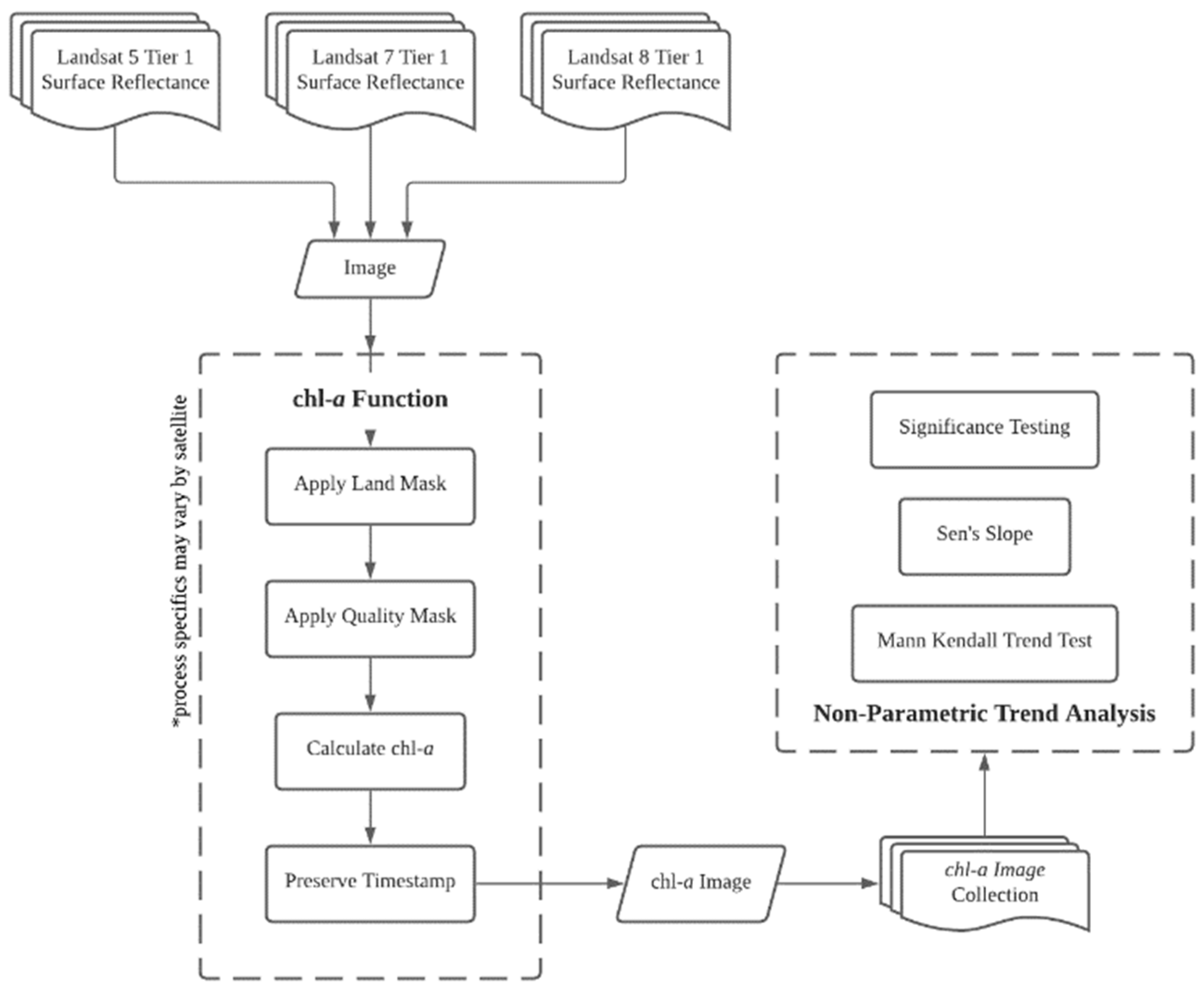
2.1. Earth Observation Data

We used the Google Earth Engine (GEE) platform to access and process the Landsat data, as GEE greatly simplifies the work required to access and process remote sensing data [48,49]. We used images from the Landsat 5, 7, and 8 missions. Landsat 5 and Landsat 7 have the same band designations, or numbered ranges of wavelengths on the electromagnetic spectrum [33]. Landsat 8, however, has different band designations (Table 1). To use published empirical chl-a concentration models for Utah Lake, we modified the models used in this study to reference the appropriate band number for each Landsat mission.
There are a number of Landsat data products (i.e., processed data) provided by NASA, including surface reflectance data. We used NASA-provided surface reflectance data that have been corrected for sensor calibration and various atmospheric effects [50,51]. These higher-level processed remote sensing products are readily accessible through GEE and eliminate the need for image calibration before processing. The NASA-processed images contain a quality assessment (QA) band, which flags pixels that are heavily clouded, have cloud shadows, or are otherwise contaminated [50]. We used this band to create pixel quality masks to exclude impaired pixels from the analysis.
For this study we estimated chl-a concentrations by applying the Utah Lake-specific whole-season empirical chl-a model based on surface reflectance developed by Hansen, Burian, Dennison and Williams [24], Hansen, Burian, Dennison and Williams [34], and Hansen and Williams [52]. This model is shown in Equation (1).
chl-a   =   e ( 1.53 + 2.55 b 5 b 1 1.15 ×   ln ( b 1 ) )
The result of this equation is the estimated concentration of chl-a in µg/L for each pixel of water in the image. To exclude bad or non-lake pixels from the analysis, we generated pixel masks based on the QA band, the presence of water, and other parameters using methods described by Cardall, Tanner and Williams [49].
This model, Equation (1), is specific to Utah Lake, and is unique because of the highly turbid water, which affects chl-a estimation. The model is based on field data from the official State of Utah Ambient Water Quality Data Management System (AWQMS). The data used to develop the model only had chl-a concentrations up to about 100 µg/L, which is below the expected maximum concentrations in the lake [24,34,52]. For pixels with very high, out-of-sample chl-a concentrations, reflectance in the blue band is very small because of how dark the water is in these locations (Figure 1). For these pixels, the blue band is the b1 term in Equation (1), and when this value is very small, the estimated chl-a concentrations become very large and are not physically plausible. To address this issue, we restricted estimated chl-a concentrations to 300 µg/L, about 3× the maximum in the data used to develop the model. This results in additional uncertainty in the higher concentration estimates, which could affect the analysis. The trend test only looks at relative concentrations, so it is less affected, and we used median, rather than mean, concentrations for most analysis, which further mitigates the impact of this uncertainty. In this study, most of the pixels, with the exception of shoreline pixels, had over 700 data points and exhibited relatively low variability, implying that the impacts from this assumption are minimal. We hold that the decision to allow the model to estimate concentration higher than the highest measured value (100 ug/L) and limit these estimates to 300 ug/L is a usable assumption for this study.
Figure 1 shows an example of this out-of-sample behavior. The left panel shows the original Landsat image using the red, green, and blue bands to simulate the visual appearance. In this image, the dark green areas in the northeast and southern portions of the lake are algal blooms. Flooding is occurring in Provo Bay, resulting in a brown plume that reaches out into the bay, with the northern, eastern, and southern portions of the bay exhibiting very brown water. The middle panel shows the estimated chl-a concentrations with values greater the 300 µg/L masked out, which results in pixels with high estimated algal concentrations not being included in the data. The brown flood waters near the shore of the bay are also masked because the algorithm determines they were land rather than water. The right panel shows the data that were analyzed in the study. The pixels with estimated concentrations greater than 300 µg/L were set to 300 µg/L. The brown, muddy pixels are still excluded, but this is a relatively rare occurrence. Other areas around the lake are masked because of low water.

2.2. Data Processing

2.2.1. Overview

We used the method presented by Cardall, Tanner and Williams [49] to process the Landsat data for analysis. This article includes processing details and example code [49]. Figure 2 presents the general steps for this approach. First, we used Google Earth Engine to generate a time-series image collection for the Utah Lake area for each of the Landsat missions (5, 7, and 8). The data in the Landsat scenes are stored as integers for space considerations. We used the NASA-supplied multipliers for each Landsat mission to convert these data to surface reflectance, renamed the bands in Landsat 8 collection to match the other collections, then merged the 3 collections into one. We then created an analysis region by drawing a polygon around Utah Lake, to exclude any local surrounding water bodies from the analysis. We next computed and applied land masks (negative water masks) to restrict the analysis to pixels representing water; applied data quality masks from the Landsat QA band to exclude pixels with cloud cover, sensor failure, or other issues; applied the mathematical chl-a model (Equation (1)) to each image pixel; and preserved the image timestamp function to allow temporal analysis. This generated a Google Earth Engine image collection of 1068 images of Utah Lake with calculated chl-a concentrations over the approximately 40-year time period of the Landsat missions, from 8 May 1984 to 24 December 2021.
We used Google Earth Engine to create summary images of the mean and median chl-a concentrations in each pixel over the study period. We excluded December, January, and February data from these mean and median images, as ice causes anomalous data and we do not expect significant algal growth in these cold months. We also created mean and median summary images for each month, i.e., average concentration in April, May, etc. These summary images are provided in the Supplementary Materials for this article. We included December, January, and February data in the other analyses unless stated otherwise.
For each individual pixel, for the lake as a whole, and for each of the analysis regions which are presented in Section 2.3, we computed time series of the mean and median chl-a concentrations and several other statistical parameters describing the data. We wrote a Python script to apply a trend test, and estimate trend slopes for each individual pixel and for each region. For both the individual pixel analysis and the analysis of the regions, the script computed the sign and statistical significance of the chl-a trend estimates using both linear regression and the Sen’s slope method, and descriptive statistics such as standard deviation, skew, and other parameters. We used Python scripts outside Google Earth Engine because the dataset was too large to compute inside Google Earth Engine.
Figure 2 and Section 2.2.2 provide detail on these processing steps. For code examples, model implementations, and implementation discussions see [49].

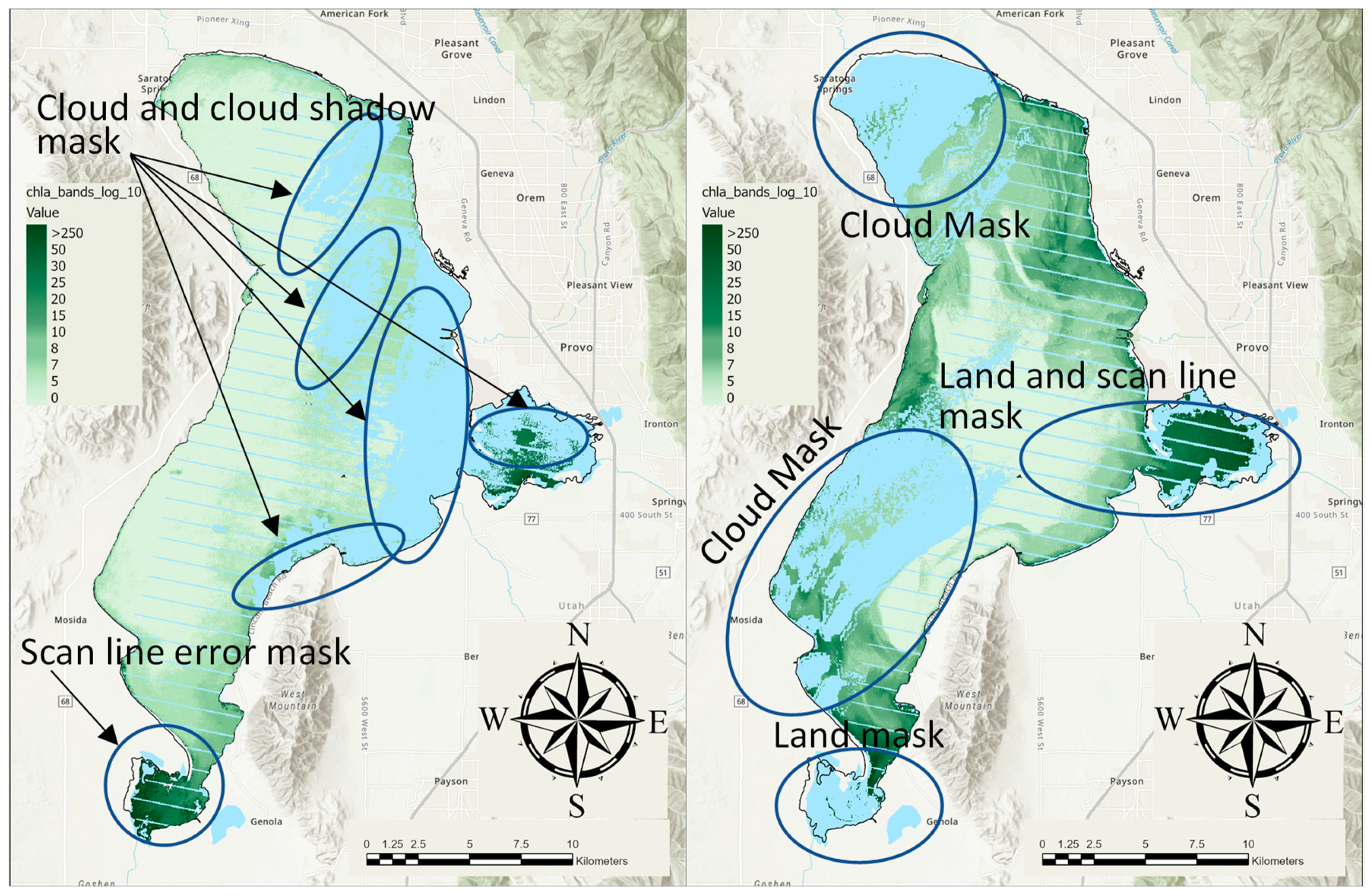
2.2.2. Pixel Quality and Water Masking Examples

Figure 3 shows examples of the masks we used to exclude pixels that contained land or had clouds, cloud shadows, or sensor issues.
We masked the regions with clouds, cloud shadows, and sensor issues using the QA band of the Landsat surface reflectance products. We generated a land mask for each image to exclude pixels that contained land from our processing. This was done in two steps: first, we created a polygon outlining the general area of Utah Lake to exclude nearby water bodies, then we differentiated between the water and land within the polygon (Figure 3) using the Modified Normalized Difference Water Index (MNDWI), which is designed to work even in turbid water or water with high algal concentrations [53]. We computed the MNDWI using the green and first short-wave infrared (SWIR1) bands:
MNDWI = Green     SWIR 1 Green   +   SWIR 1
We excluded pixels that had an MNDWI value greater than 0.95, then used the negative of this mask to create a land mask which excluded non-water pixels (Figure 3). Using the land mask on each image in the collection captured Utah Lake’s dynamic shoreline, which changes significantly with varying lake elevations.
Figure 4 shows the total number of pixels analyzed at each point in the Lake, with low numbers around the shoreline, Bird Island, and the shallow bays reflecting low water levels and land exposure that occurred during the study period. While the image collection consisted of 1068 images, many of the images had areas that were masked, and some images had no usable lake pixels. The central area of the lake generally had over 600 usable measurements at each pixel, while Bird Island, the shallow bays, and the shoreline had significantly fewer measurements because they were not covered by water when many images were collected.
In Figure 4, pixels with no data points are transparent, revealing the underlying background map. Selected areas in Utah Lake are highlighted to demonstrate how land masking affected data processing. The pixel counts around Provo Harbor (top insert in Figure 4) clearly show breakwaters and dock structures. Figure 4 shows the area around Bird Island (second panel from the top) with the center transparent, as it remained exposed for the duration of the study period, and the surrounding areas with low counts because of years with low lake level which exposed larger areas of the island. Figure 4 also shows Provo Bay and Goshen Bay, the second from bottom and bottom panels, respectively. These bays are shallow and change size significantly depending on lake levels. Figure 4 clearly shows this effect, with the boundaries of these bays having fewer pixels available for analysis than the centers, which have numbers similar to the rest of the lake. These pixel counts indicate that the water/land masks were effective and inform our analysis of chl-a trends in shallower areas.

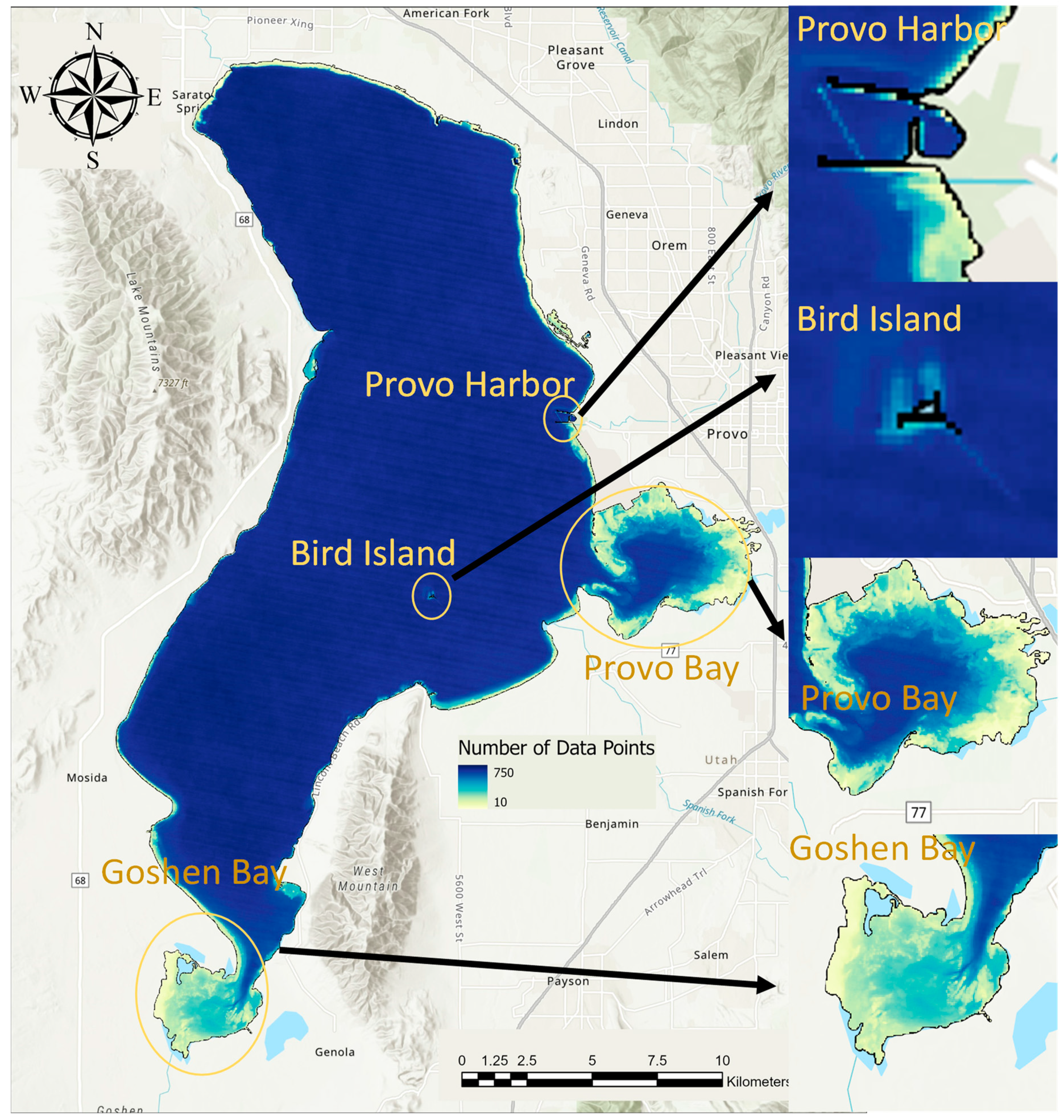
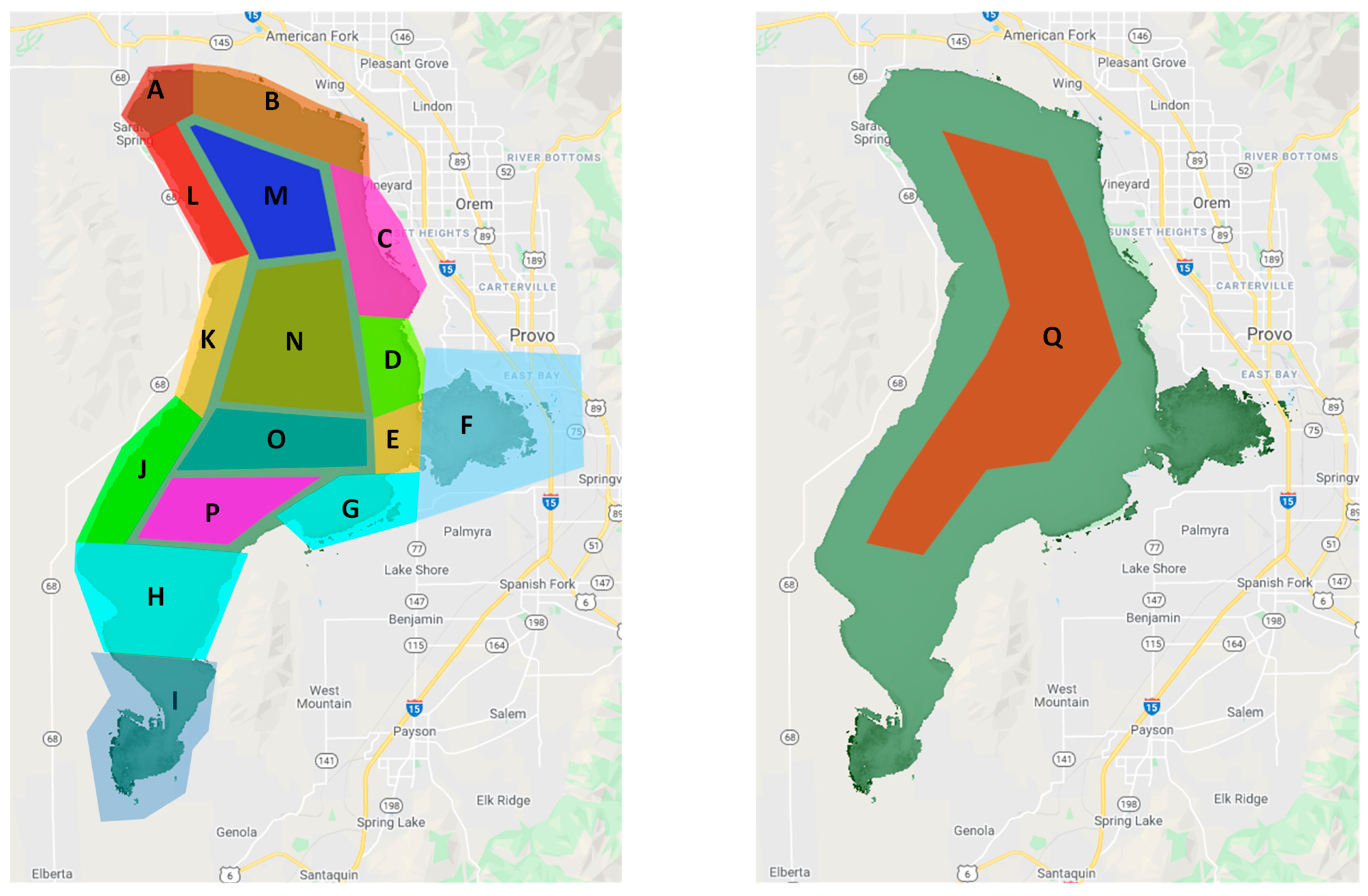
2.3. Utah Lake Analysis Regions

To attempt to identify and characterize impacts from WWTPs, river inflows, near-shore development, watershed changes, and other spatially varying impacts on Utah Lake, we divided the lake into several different regions for statistical analysis (Table 2 and Figure 5). We selected these regions to isolate areas of the lake that could be most influenced by various inflows, outflows, and shoreline uses. In addition to these regions, we computed the statistics for the entire lake and for each pixel.
When computing chl-a concentrations for any image, only the pixels that were not masked were used. This means that the size of the regions that contain shoreline, as well as the entire lake, was potentially different for each image in the time history, resulting in a different number of pixels analyzed for each time step. Figure 4 shows the total pixel counts for the study period. Any pixel may or may not have been present at a given time step for which regional statistics were computed.
The regions and their selection criteria are summarized in Table 2. The lake is very large (40 km × 21 km) and shallow (~2–3 m), with the depth being essentially constant over the lake—the shallowest areas are Provo and Goshen Bays, and the deepest water is in the center of the lake and near the Jordan River outfall (Figure 5, Region A), which reaches about 3–4 m at high pool conditions. Outflow is only ~50% of inflow, with the remainder lost to evaporation based on mass balance calculations [54]. In addition, underwater seeps and springs provide an unknown, but significant, inflow, indicating that evaporation accounts for more than 50% of the surface inflow [54]. This extreme size, shallow depth, and limited outflow suggest that lake is not well mixed and these selected regions may behave differently from one another if they are significantly influenced by the shoreline processes, inflows, or outflows.
Region A contains the Jordan River outfall. This is the only outlet for Utah Lake. Most of the north and east shoreline areas (regions B and C) are pasture or swamp lands and contained the Geneva Steel plant, which is being decommissioned. Region B contains both the American Fork and Lindon Marinas and is relatively undeveloped near the lake. Housing development in Region C started about 5–10 years ago, prior to that the area was agricultural and pastureland. Region D contains Provo Harbor, the most active marina on the lake, and the discharge point for the Provo River which is the main tributary to the lake. About 2 years ago restoration construction on the Provo River delta commenced and is now almost complete. Provo Bay (Region F) exhibits different characteristics from the rest of the lake: it is less turbid and surrounded by wetlands. It receives inflow from Hobble Creek and several other small streams. The Provo and Springville WWTPs discharge into Provo Bay. About 10 years ago, a restoration project on Hobble Creek altered the flow patterns, increasing the flow in Hobble Creek and allowing it to discharge directly into the bay. Region E, at the mouth of Provo Bay, also exhibits slightly different characteristics from the lake, with less turbid water as the relatively clear water from Provo Bay enters the lake. Region G is pastureland on the shore with little development. It receives discharge from the Spanish Fork WWTP. Region H is the southern portion of the lake. The shore in this area contains some pastureland on the east, with the central portion containing orchards. The western shore is a dry desert landscape. This region contains numerous seeps and springs. One large spring creates Bird Island, a carbonate deposit actively maintained, about 1 mile offshore. The lakebed between the shore and Bird Island is a hard carbonate substrate with shallow water (<1 m) in many areas. Region I is Goshen Bay, this is a shallow bay surrounded by orchards and agricultural land. The bay is often dry in low water years and very shallow in wetter years. Because of the shallow water, plants grow in the bay, which can interfere with chl-a estimates. The shoreline of region J is a desert landscape with little to no development and no streams or seeps, though there might be seeps in the lake. Region K is a desert landscape, like region J, but in the last 10–15 years housing development has occurred, with housing very near the shore. Region L has some seeps and springs, but no streams or creeks. The small town of Saratoga Springs is in this region. In the last 15–20 years, this area has been significantly developed, with housing close to the shore. Regions M, N, O, and P represent center sections of the lake away from shoreline influences. Region Q represents the center of the lake.
These regions represent a variety of conditions on Utah Lake. Regions B, C, and F receive significant effluent from WWTPs, while region G receives effluent from a smaller plant. The regions on the north and east of the lake were green agricultural regions that were mostly pastureland that was both irrigated and naturally wet from the high groundwater table and seeps; these areas have undergone significant development in the last 10–15 years. The regions on the west of the lake have essentially desert shorelines, with few green areas, through the extreme south end of the lake is bordered by irrigated fields. The northwest portion of the shore is undergoing rapid development, but only the extreme northwest corner was developed historically. There are no perennial streams on the west side and all WWTP effluent from the developed regions on the north and west of the lake is discharged into the northeast portion of the lake (Region B).
The variety of the regions in terms of potential inflow impacts and lake processes, the different infows to each region, and the slow mixing of the lake allow us to evaluate long-term trends and determine if different regions exhibit different histories, which we can then use to determine potential correlations between chl-a concentrations and WWTP effluents, shoreline development, watershed changes, and other factors. By characterizing both the entire lake (i.e., individual pixels) and lake regions, we can gain insight into how historical events and conditions have impacted water quality, as indicated by chl-a concentrations. This has implications for future management decisions, as this study can reveal the sensitivity of the lake to various inflows and other factors.

2.4. Trend Analysis Methods

To determine historical trends in algae growth on Utah Lake, we used the Mann-Kendall (M-K) test [55]. The M-K test is commonly used to identify monotonic trends in environmental, climate, and hydrologic data and is recommended by the US EPA National Nonpoint Source Monitoring Program [56]. The M-K test is a non-parametric statistical test, which is ideal for this analysis because it is not affected by missing data or the data distribution. As any individual pixel can be contaminated by clouds or other issues, the data streams do not have a consistent spacing or a consistent number of data points. The M-K test determines if the data exhibit increasing, decreasing, or no trends and whether these trends are statistically significant. We applied the M-K test to individual pixels, and to the time series of statistical values computed for each defined region.
The M-K test null hypothesis, H0, is that the data come from a population with independent realizations and are identically distributed–in other words, there is no trend. The alternative hypothesis, HA, is that the data follow a monotonic trend. The M-K test statistic is calculated as:
S = k = 1 n 1 j = k + 1 n sgn ( X j X k )
with:
sgn ( X j X k ) = { 1   if   ( X j X k ) > 0 0   if   ( X j X k ) = 0 1   if ( X j X k ) < 0
where S is the M-K statistic, n is the number of samples and Xi is the ith sample. The M-K test evaluates every potential pair of measurements and sums the sign of the difference. If every one of the 1068 images in the historic data were included in the analysis of a particular pixel, then the number of pairs is 569,778, or over 0.5 million samples for each pixel, which would need to be evaluated to compute S for that pixel.
When S is a large positive number, values later in the series tend to be larger than values earlier in the series, indicating an upward trend. When S is a large negative number, later values tend to be smaller than earlier values, indicating a downward trend. A small absolute value of S indicates no trend. M-K normalizes S to allow comparison with other data sets.
The normalized M-K statistic, τ, is computed as:
τ = S n ( n 1 ) 2
which has a range of –1 to +1. Positive and negative values indicate the likelihood of increasing or decreasing trends, respectively. The normalized test score allows comparison with other data sets with the magnitude of τ and S indicating the likelihood of the trend.
To determine if the null hypothesis of no trend can be rejected, the ZMK statistic is computed [57]. First, the variance of S is computed as:
V ( S ) = ( n ( n 1 ) ( 2 n + 5 ) ) ( p 1 g t p ( t p 1 ) ( 2 t p + 5 ) ) 18
with the ZMK test statistic computed as:
Z MK = { S 1 V ( S )   if   S > 0 0   if   x = 0 S + 1 V ( S )   if   S < 0
where V(S) is the variance of S, g is the number of tied groups, and tp is the number of observations in the pth group. The value of ZMK is compared to the significance level, in our case 0.05, to determine whether to accept or reject the null hypothesis at the selected significance level. ZMK is analogous to p values reported in many statistical studies.
It is important to emphasize that the M-K test does not estimate or determine the magnitude of a trend, only the likelihood that a trend exists and whether it is increasing or decreasing. We used the M-K test to characterize temporal trends in algae concentration in Utah Lake and determine if those observed trends are statistically significant or if they could be explained by chance.
We estimated the trend or rate of change using two different methods, a linear least squares fit and the Sen slope estimator. The Sen’s slope estimate is computed as [58]:
β 1 = median ( y j y i x j x i )
for all i < j and i = 1, 2, …, n − 1 and j = 2, 3 … n. The Sen slope estimator is the median slope for all data pairs used to compute S in the M-K analysis. If a pixel has values in all 1068 images, then this would be the average of 569,778 pairs; however, most pixels had about 650 values, which is over 200,000 pairs.
We used the pymannkendall package (ver 1.4.2), from conda-forge to compute the M-K statistic for both individual pixels and for the regional time series data [59]. This code includes a Sen Slope estimator routine. We modified the Sen Slope code to use time stamps rather than assuming the data were sampled on regular intervals and modified the output to generate slope as change-per-year, rather than change per time step.
We used the linalg.lstsq function from the python numpy package to fit a linear least squares line to data and find the resulting slope [60]. We report the linear least squares slope as change-per-year, comparable to the Sen’s slope value.

3. Results

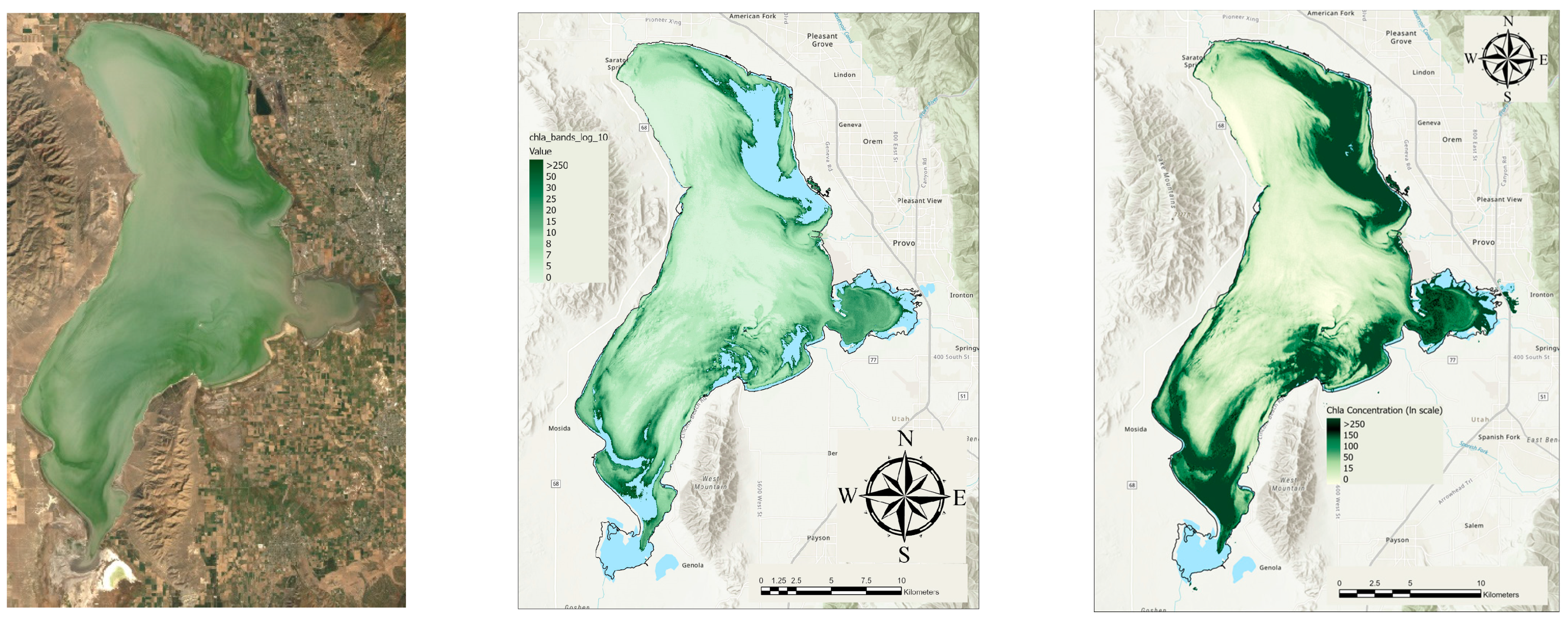
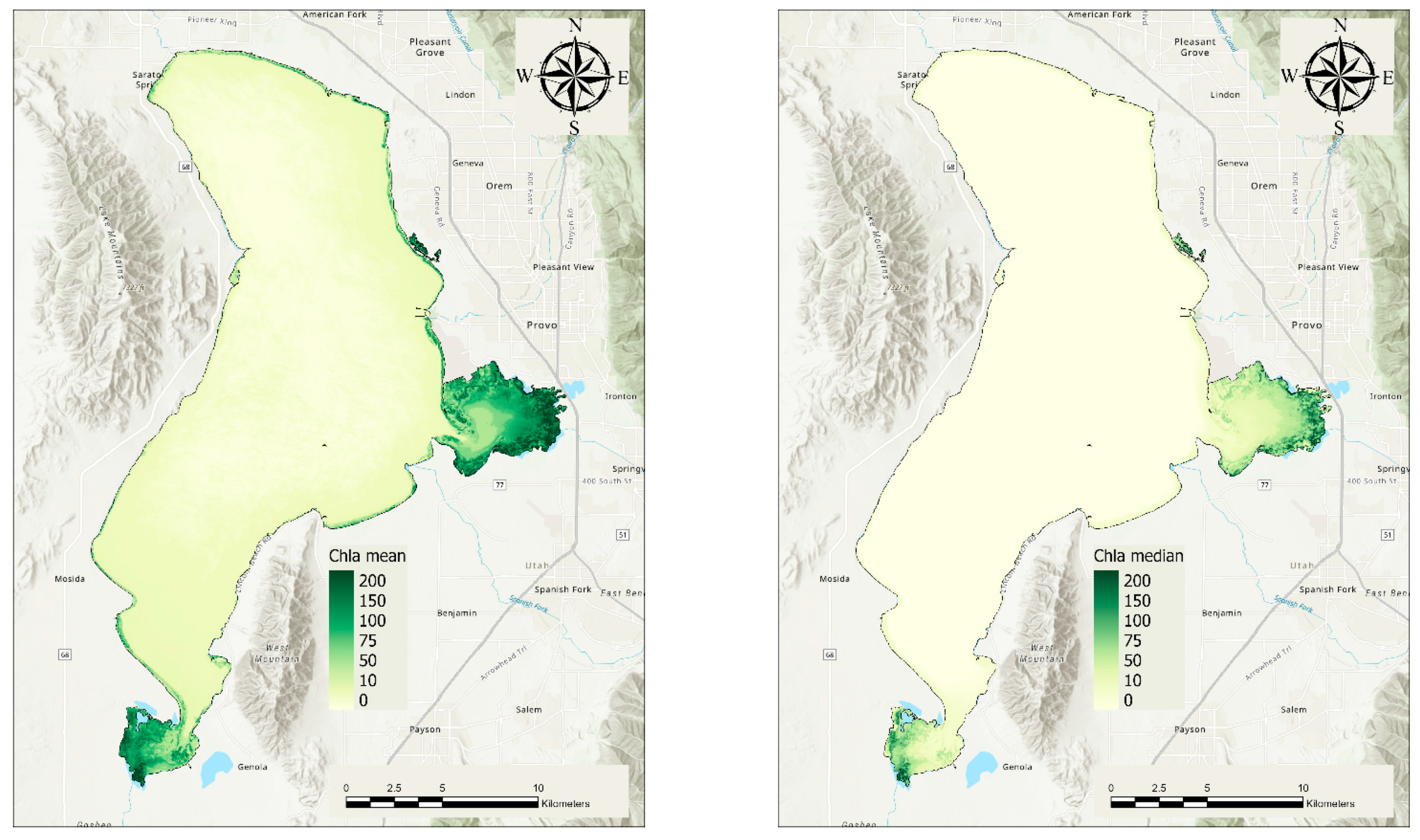
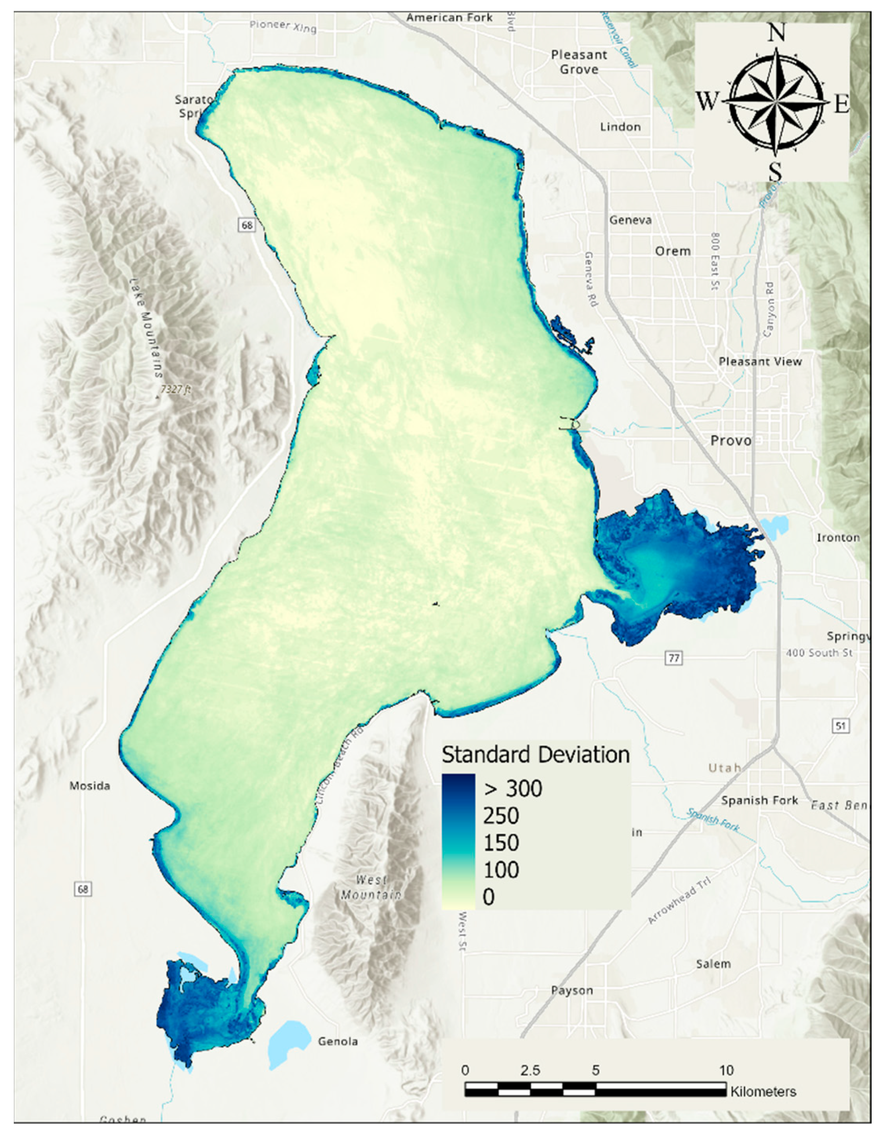
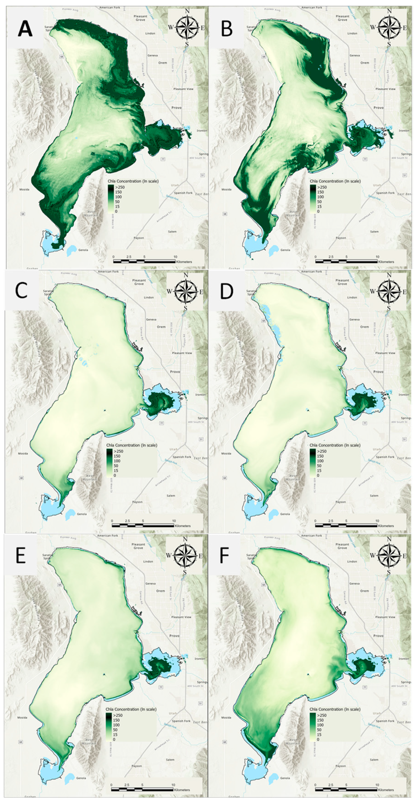
3.1. Average Chl-a Concentrations

Figure 6 presents the mean and median chl-a concentrations for each image pixel computed over the ~40-year study period. Our data have high concentration outliers which skew the mean values higher, as can be seen in Figure 6, where the mean values (left panel) are noticeably higher than the median values (right panel). The color scale in Figure 6 is non-linear and designed to highlight differences in the lower concentration regions. For example, the colors range from light yellow through green for the 0 to 50 µg/L range but only change from green to darker green for the entire range from 50 to 200 µg/L. The quantitative difference in chl-a concentrations is not as large as the visual representation. The electronic supplement contains mean and median spatial distribution images for each month over the ~40-year period. For the majority of our analysis, we used the median values because they are more indicative of the central tendency of data that have outliers [61].
Most of the lake exhibits a very low median value over the duration of the study period: less than 5 µg/L. Concentrations are generally higher on the east side of the Lake, with median concentrations in that area typically below 10 µg/L. The two shallow bays, Provo Bay on the central east shore and Goshen Bay on the south end, exhibit significantly higher median concentrations over the long study period, with the periphery having median values over 200 µg/L. The median values at the edges of these bays may be higher because of the impact of shallow water vegetation on the estimates. The interiors of these bays also exhibit high median values, generally over 50 µg/L with large areas of the bays over 70 µg/L, with mean values of over 150 µg/L and 200 µg/L, respectively. The shoreline areas around Provo Bay, both to the north and south of the entrance, show higher median and mean values, with concentrations greater than 175 µg/L and 250 µg/L, respectively, and the area immediately near the mouth shows median and mean concentrations greater than 30 µg/L and 70 µg/L, respectively.
Figure 6 shows that while high concentrations do occur on the open lake, on average the concentrations are generally low. The eastern shore exhibits slightly higher concentrations, possibly due to prevailing winds which push algal blooms to the shore. The southern third of the lake also exhibits slightly higher mean and median values, which we attribute to blooms moving from Goshen Bay into the lake. This region is narrow and does not provide much mixing. The area immediately around the mouth of Provo Bay exhibits similar behavior, though this region of higher concentrations does not extend as far into the lake as that of the mouth of Goshen Bay.
Water flows from Provo Bay into the main body of Utah Lake. Our data suggest that the higher values around the mouth of Provo Bay are because of water with high chl-a concentrations moving from Provo Bay out into the Lake, rather than local processes creating conditions that support higher phytoplankton growth. Areas around the mouth of Goshen Bay exhibit a similar pattern, though some of this may be wind-driven.
The shallow bays have significantly higher mean and median chl-a concentrations than the rest of the lake. While we cannot attribute these concentrations to any specific physical process, the shallow water is probably warmer on average than the remainder of the Lake. In addition, there are indications that Provo Bay is not as turbid as the remainder of the lake. Data available in the official State of Utah Ambient Water Quality Data Management System (AWQMS) water quality database show that nutrient concentrations in Provo Bay are generally lower than those in the main body of the lake, so nutrient levels alone are not likely to be the cause of these higher mean and median values. Studies indicate that phytoplankton growth in Utah Lake is most likely light limited [2], so the less turbid water in the bay may facilitate increased algal growth and therefore higher chl-a concentrations.
Goshen Bay is not less turbid than the general lake, but is much shallower than Provo Bay, which could be the reason behind the higher observed chl-a concentrations. We do not have enough data to compare nutrient levels in Goshen Bay to the lake body.
Figure 7 shows the standard deviation of the chl-a data over the study period. These data are not normally distributed, but the standard deviation values provide a representation of the variability of the data. As in Figure 6, the color scale for Figure 7 was selected to highlight small differences in the body of the lake, with the change from light yellow to green to blue occurring from 0 to 100 µg/L, and from 100 to over 300 µg/L being represented as lightly blue to dark blue. This color scale does not highlight the detail in regions with higher standard deviation in the two shallow bays.
The body of the lake, shown in light yellow, has low variability—typically less than 10 µg/L—with higher variability of between 50 to 100 µg/L on the eastern and northern shores shown as light green. The areas near the northwest center of the lake and more limited areas near the central west portion of the lake have the lowest standard deviations. We attribute this to lake currents and winds that affect the remainder of the lake. In the southern and eastern portion of the lake, there are currents that bring water with high chl-a concentrations from Goshen and Provo Bays, and prevailing winds tend to push algal blooms generally north and east, causing higher variations in these areas. Both Provo Bay and Goshen Bay have very high variability, which we attribute to the frequent algal blooms that occur in these bays and to changing water levels. Provo Bay shows different variance in different areas. The lower standard deviation near the center and mouth of Provo Bay we attribute to the fact that chl-a levels in Provo Bay are consistently high, and do not exhibit as much deviation. The larger variations near the shore and in the eastern end of the bay we attribute both to low water years changing the shoreline and prevailing mid-morning winds, which often drive surface phytoplankton to the eastern shore around the time that Landsat collects an image of Utah Lake (10:30 A.M. local time).
To highlight some of these lake processes, Figure 8 shows the chl-a concentration distribution for selected dates. Panels A and B show large lake-wide blooms, panels C and D show a bloom developing and flowing out of Provo Bay over a 16-day period, and panels E and F show blooms developing and flowing out of both Goshen Bay and Provo Bay over a 16-day period. We selected these images to demonstrate various conditions that occur in the lake. Water levels in Utah Lake vary both based on annual precipitation and the time of year. Panels A and B show the lake relatively full, while panels C-F show low lake levels with Goshen Bay nearly dry and Provo Bay significantly reduced in area. Utah Lake is an actively managed reservoir that is generally full in the late spring and early summer and low in the late summer and early fall, though in low-water years it can be low in the spring.
Figure 8 shows that while long-term mean or median values in the lake body are low, high-concentration blooms do occur. Panel A of Figure 8 shows an algal bloom occurring along the northeastern shore, as well as water with high chl-a concentrations from Goshen Bay being pushed out into the Lake. Panel B shows a similar bloom. Based on the patterns in the concentration, it appears that the blooms are beginning in Goshen and Provo Bays, then moving north along the eastern shore towards the outfall in the northwest corner of the lake. While this appears to be a continuous bloom, panels A and B are typical of the bloom patterns most often seen on the lake: isolated blooms occurring in multiple locations and moving over time. Even with these large periodic blooms, the majority of the lake generally exhibits low concentrations.
Panels C and D show a bloom developing in Provo Bay over a 16-day period. These blooms are common and indicated by Figure 6. These maps show water with high chl-a concentrations flowing out of Provo Bay into the larger lake body. Panels C and D show a smaller bloom originating in Goshen Bay, also moving out into the lake. This flow pattern may be the reason behind the higher median and standard deviation values in the areas near the mouth of Provo Bay and in the southern third of the lake. Panels E and F show similar blooms developing over a 16-day period in both Goshen and Provo Bays, in both areas the blooms appear to be moving out of the bays, into the lake, and northward towards the outfall.

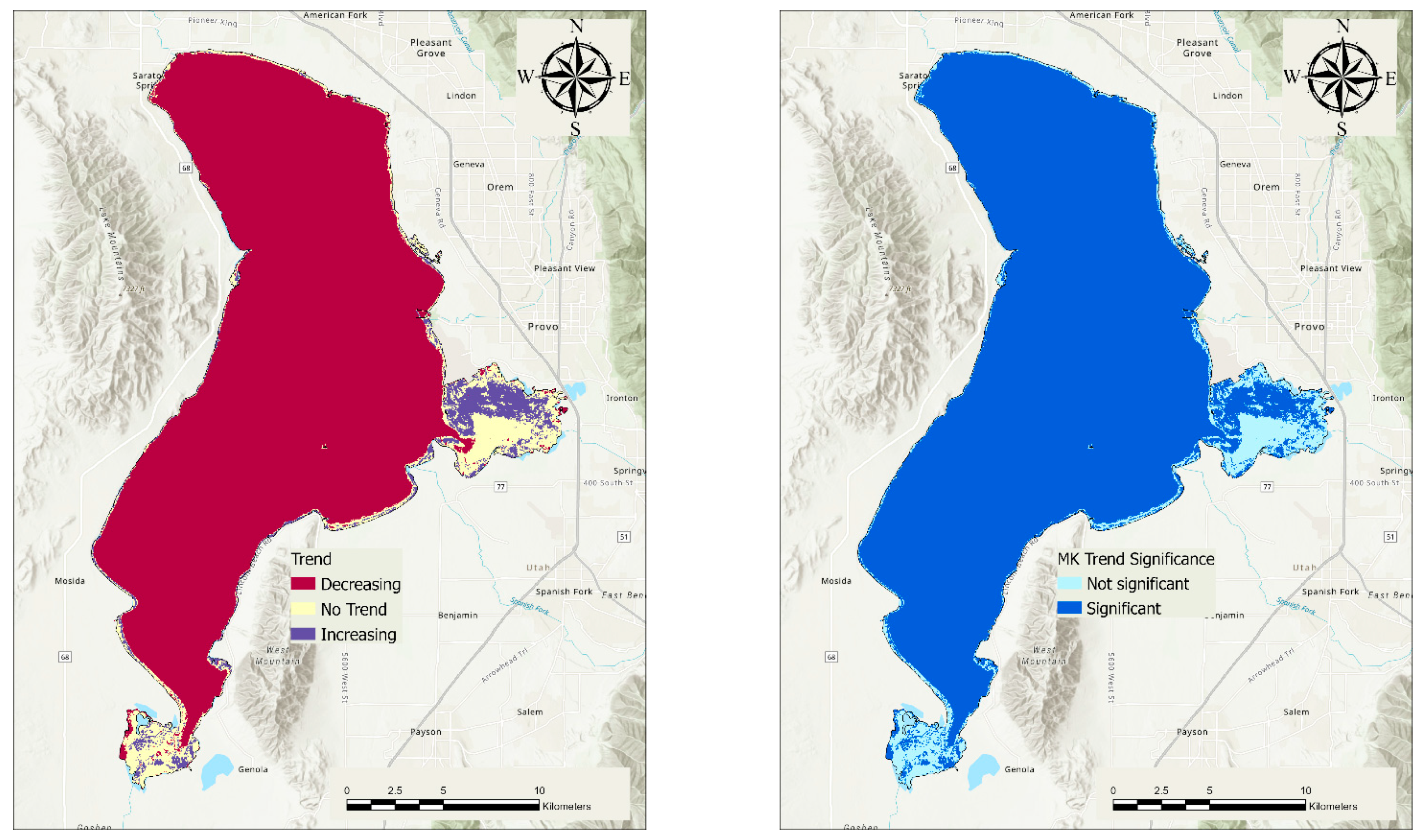
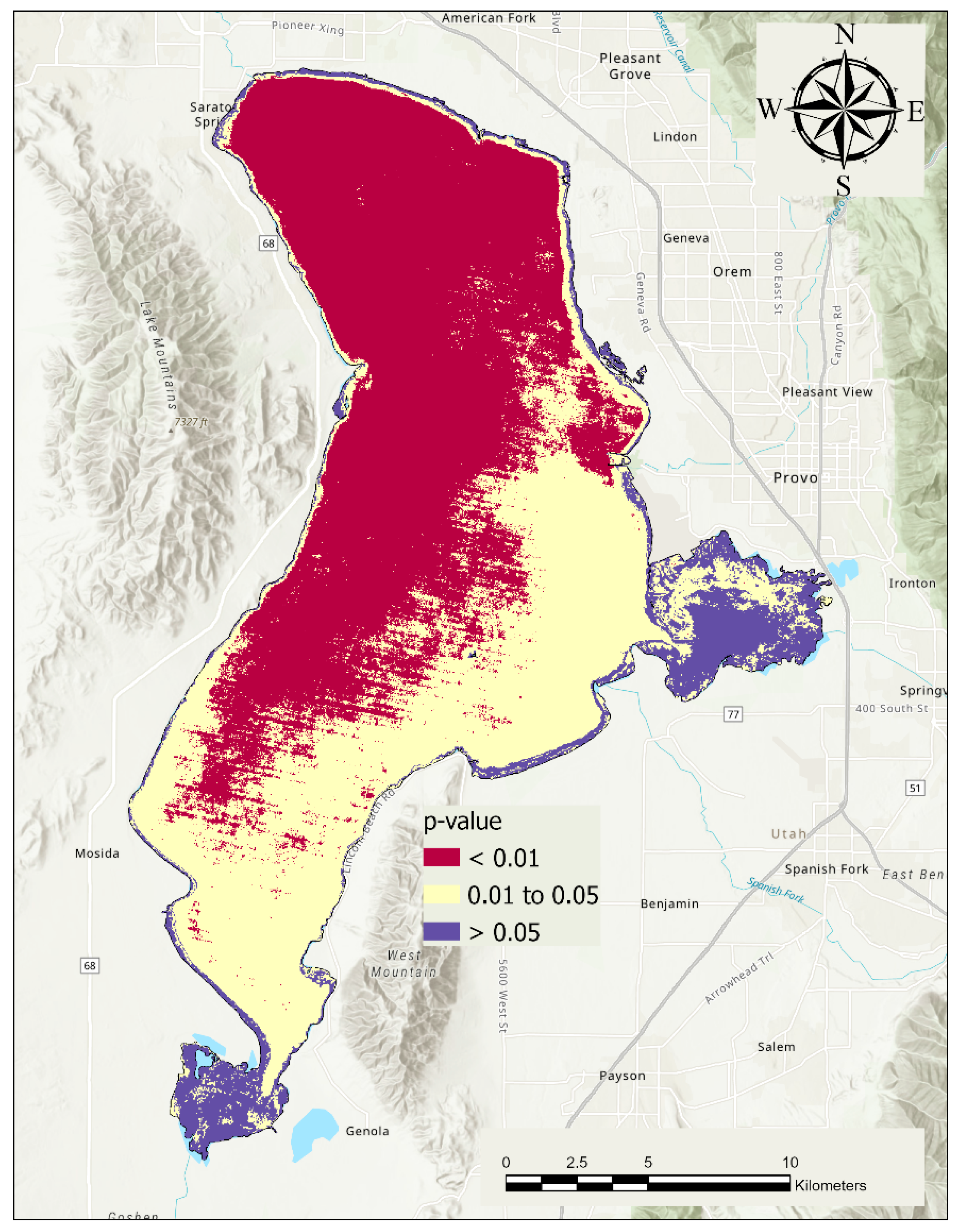
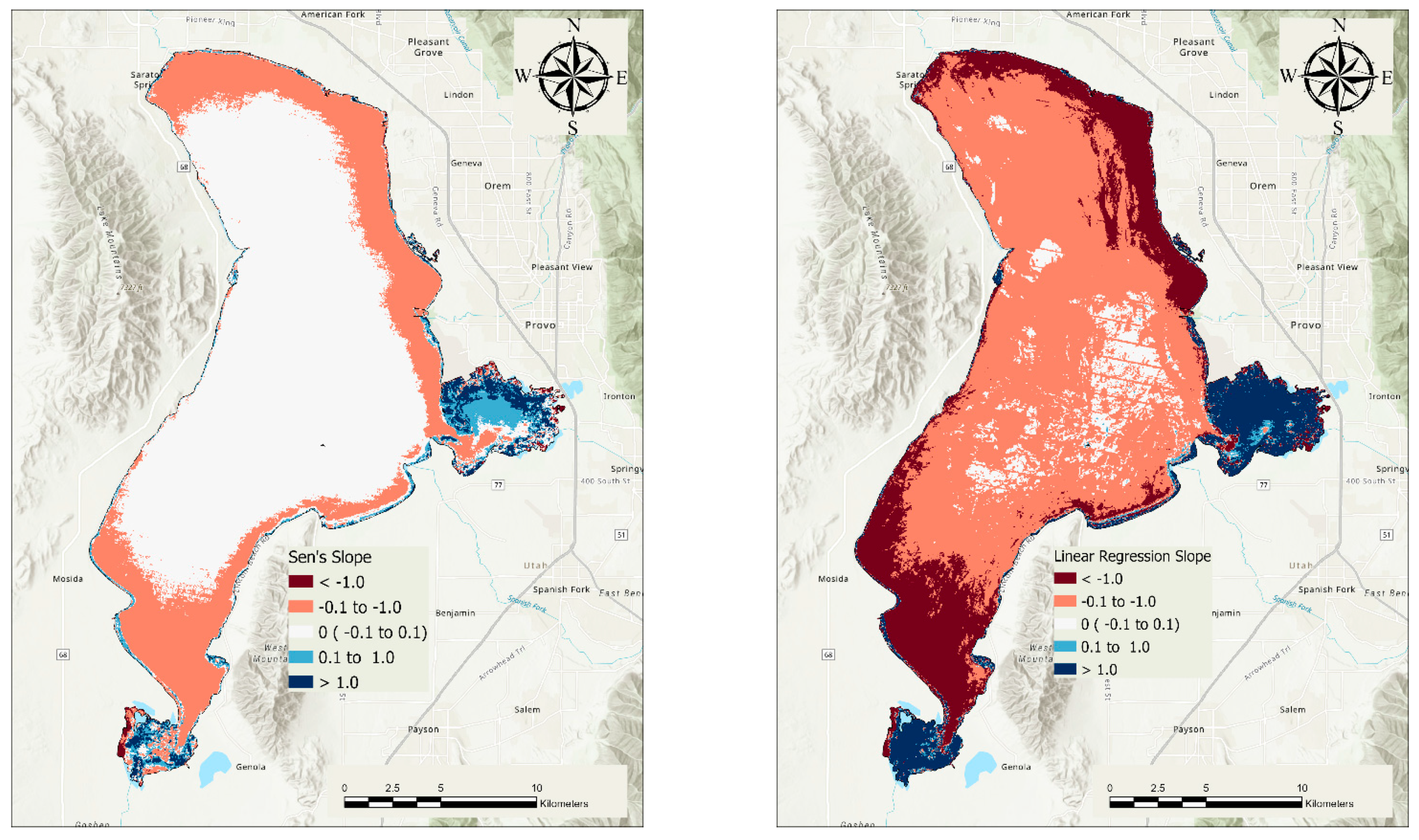
3.2. Trends in Chl-a Concentrations

Figure 9 shows the results of the trend analysis for each pixel over the study period. The left panel of Figure 9 shows whether each pixel has an increasing trend, a decreasing trend, or no trend based on the M-K test, and the right panel indicates whether these trends are statistically significant at the p-0.05 level (Figure 10). Trends that did not meet the required p-value are labeled as “no trend”, as there is no statistically significant trend in these pixels. For nearly all pixels in the lake, with the exceptions of Provo Bay and Goshen Bay, the computed M-K trends are statistically significant, although this is partially because of the large number of data points available for analysis at each pixel (Figure 4).
Figure 9 shows that, for the majority of the Lake, chl-a concentrations have a decreasing trend over the ~40-year study period, with the areas near the mouth of Provo Bay exhibiting no trend. Provo and Goshen Bays both exhibit increasing trends in chl-a concentrations, with significant areas in both Bays not having statistically significant results, likely due to the high variability of the data in those areas (Figure 7).
Figure 10 shows the distribution of p-values used to determine if the M-K trends shown in the left panel of Figure 9 were statistically significant. The statistical significance map (right panel of Figure 9) is based on these p-values. The map shows areas with p-values of 0.01, 0.05, and greater than 0.05 as maroon, yellow, and purple, respectively. This shows that the decreasing trends computed in the northwest portion of the lake have less than a 1% probability of occurring randomly. The trends computed for the remainder of the lake, with the exceptions of Provo Bay and Goshen Bay, have less than a 5% chance of occurring by chance.
The M-K test does not compute a quantitative value for the trends; only if the trend is increasing or decreasing and if the trend is statistically significant. We estimated trend values for each pixel using two methods: Sen’s Slope and by fitting a linear regression line with the results shown in the left and right panels of Figure 11, respectively.
Figure 11 shows that while the decreasing trends in the majority of the lake and the increasing trends in the north portion of Provo Bay and a few pixels in Goshen Bay are statistically significant, the magnitude of these trends is so low that they have no discernable impact on the lake. Most of the lake has slopes with decreasing magnitudes of less than 0.05 and 0.005 µg/L/year for the Sen’s slope and linear regression slope, respectively. The left panel of Figure 11 shows that the north-eastern shore has more negative slopes, with slightly higher magnitudes of Sen’s slope, decreasing at rates up to 0.1 µg/L/year. Over a ~40 year-period, these slopes would result in decreases of 2 to 0.2 µg/L over the study period for the 0.05 and 0.005 values, respectively. These changes are much smaller than the standard deviation in these regions. Figure 11 shows increasing slopes in Provo Bay with values of about 0.1 and 0.005 µg/L/year for Sen’s slope and the linear regression slopes, respectively. These trends would result in increases of 4 and 0.2 µg/L over the study period for the Sen’s slope and linear regression slope estimate, respectively. These changes are inconsequential compared to the natural variability in the lake but are statistically significant trends.
Our trend analysis shows that while there are statistically significant decreasing and increasing trends for the lake and the bays, respectively, these trends are small and inconsequential in terms of chl-a concentrations. Chl-a concentrations exhibit large variability both spatially within the lake and temporally throughout the duration of the study period, significantly larger than any changes that would result from the estimated trends.

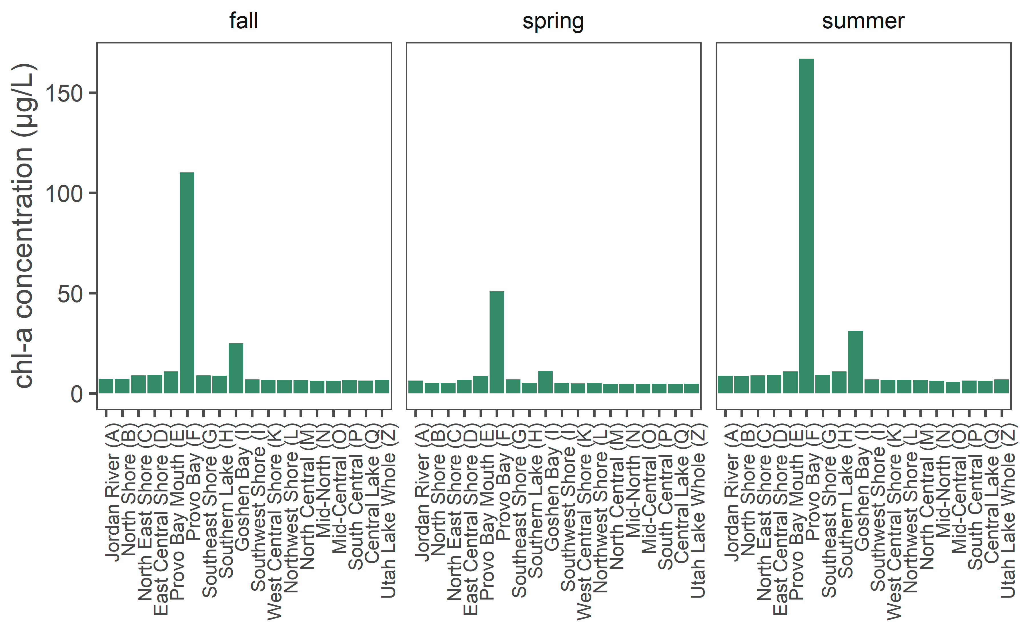
3.3. Regional Trend Analysis

To further illustrate lake behavior, in Figure 12 we plotted the median, 25th, and 75th percentile values for the Jordan River region (the region that contains the lake outfall), Provo Bay, and the whole lake. Figure 12 only includes data from March through November. We did not include data from the winter months, as the lake is typically frozen and not many pixels are available for these months. The plots include the median values for each region shown as a black line, and the 25th and 75th percentile ranges as a filled backgrounds to highlight the spread of the data.
These plots show the large variability of the data, the difference among regions, seasonal patterns, and differences between wet and dry periods which cause lake levels to fluctuate. The electronic supplement contains plots for the other analysis regions. Figure 12 shows that in the late 1980′s there were large spikes in algal concentrations. These spikes correspond to the large algal bloom shown in Figure 1 and the top panels in Figure 8.
Table 3 presents the results of the M-K test applied to chl-a estimates for the data from March through November for each analysis region (See Table 2 and Figure 5 for descriptions of these regions). All these trends, except for Provo Bay, are decreasing and statistically significant with p-values less than the threshold value of 0.05. The p-value for Provo Bay is large, 0.42, compared to the threshold value of 0.05, indicating that the data exhibit no trend.
Except for Provo Bay (F), all regions have very small statistically significant decreasing trends, with Sen’s slope values of less than 0.1 µ g/L/year, with the exception of Goshen Bay, which has a value of −0.48 µg/L/year. Slopes of this magnitude result in minimal changes over the 40-year period. Provo Bay (F) has no statistically significant trend and has an estimated Sen’s slope of 0.07 µg/L/year, though the estimated linear regression slope for Provo Bay is 0.83 µg/L/year, much larger than any of the other computed slopes though similar in magnitude to the large negative slope in Goshen Bay.
The trends in all regions except Provo Bay (F) are statistically significant based on a 95% confidence limit (p-value < 0.05); all the regions have over 850 data points (i.e., images with usable pixels in the region) over the study period, allowing most statistical tests to be significant, even though the very low Sen’s slope and linear regression slope values indicate there is essentially no trend for any of the regions because the slopes are so small.

3.4. Lake Region Comparisions

Although the magnitudes of the trends in all regions except Provo Bay are very small, there are large differences in the average chl-a concentrations in different regions (Figure 13). We performed a Kruskal–Wallis multiple comparison of means test on the data from each region, which gave a p-value of 2.2 × 10⁻¹⁶, indicating that some of the differences in average chl-a concentrations between regions are statistically significant.
Figure 13 illustrates the median chl-a value for each region by season, with the first panel representing the fall months (September through November), the second panel representing the spring months (March through May), and the last panel representing the summer months (June through August). In each panel, each region is represented by a bar, with the height corresponding to the median chl-a value during that season over the study duration.
Figure 13 shows that regions F (Provo Bay) and I (Goshen Bay) have the highest average chl-a concentrations. Areas E (Provo Bay Mouth) and G (Southeast Shore) are the next highest and are both near Provo Bay. Areas C (Northeast Shore) and D (East Central Shore) have slightly higher levels. Since these areas are just north of the Provo Bay entrance in the direction of water flow and prevailing wind, this supports visual observations (Figure 8) that water with high chl-a concentrations flows out of Provo Bay and moves north along the eastern shoreline towards the lake’s only outflow. The slightly higher values in the Southern Lake region, at the mouth of Goshen Bay, indicate a similar pattern, though less pronounced.
Figure 14 shows how the mean chl-a value for the whole lake varies with the season, starting with low values in the spring (March–May), increasing in the summer (June–August), and decreasing slightly in the fall (September–November), but not as low as the initial spring values. This illustrates the high variability of average chl-a concentrations in the lake during the fall and summer, which is likely a function of intense but brief algal blooms and the impact of high and low water years on algal growth.

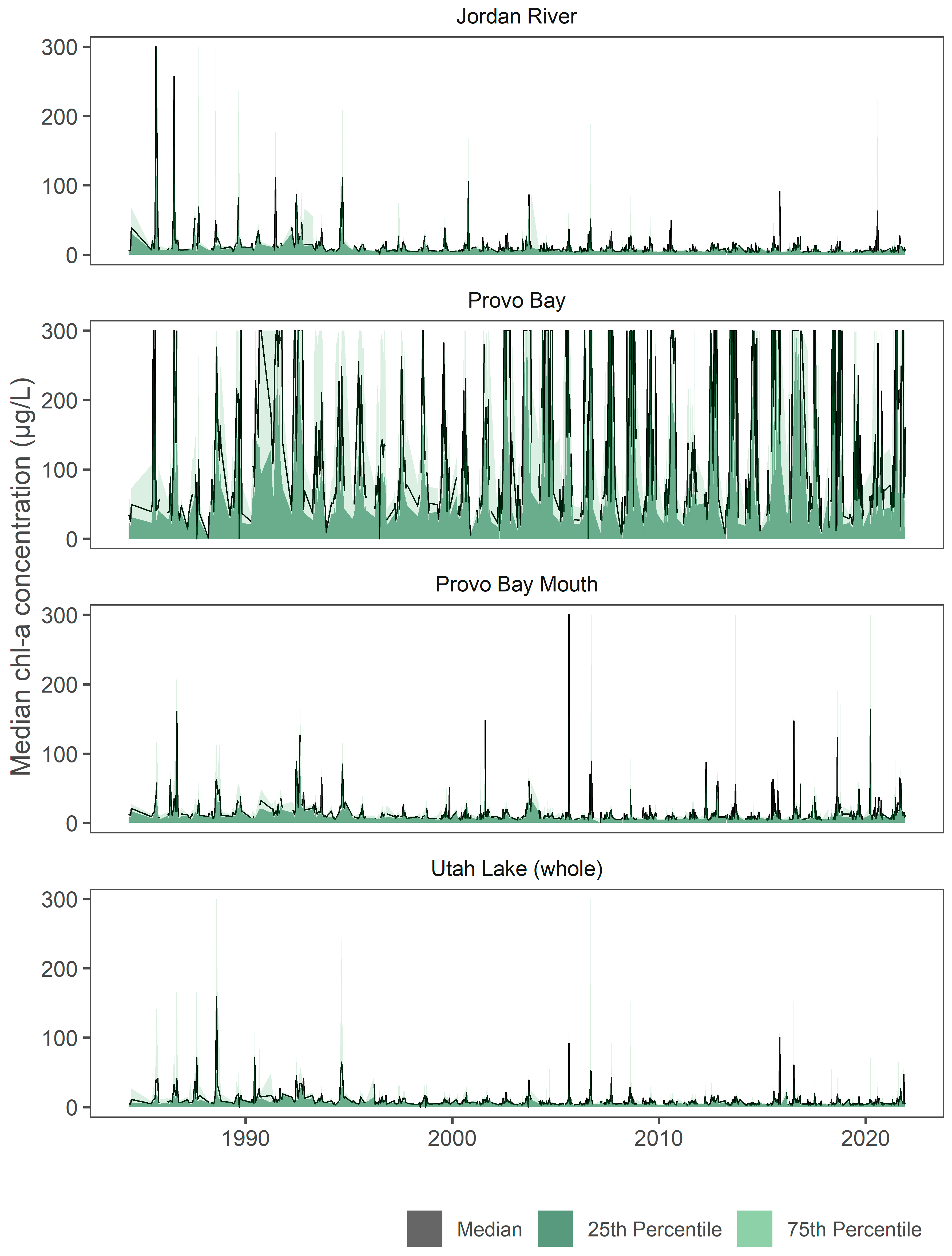
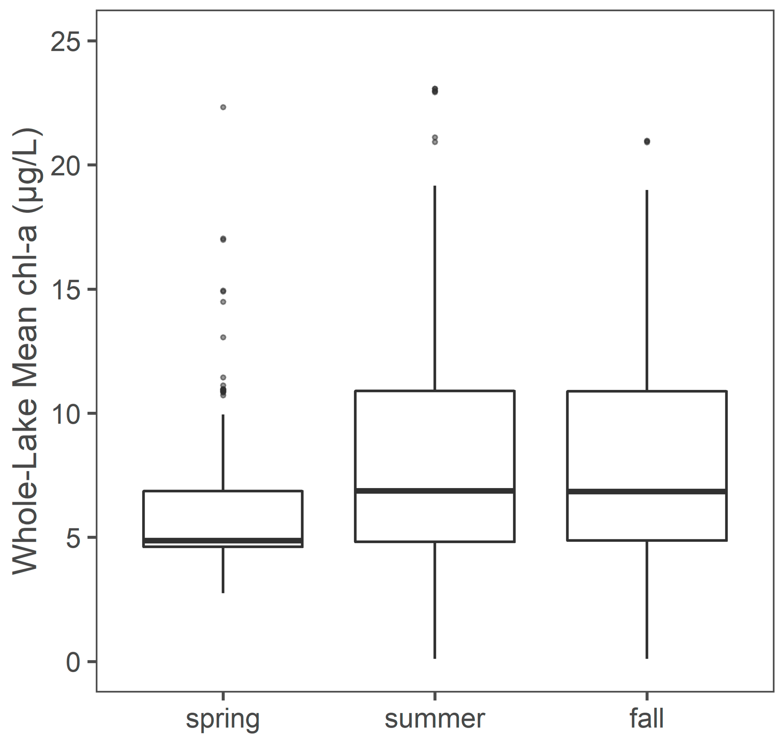
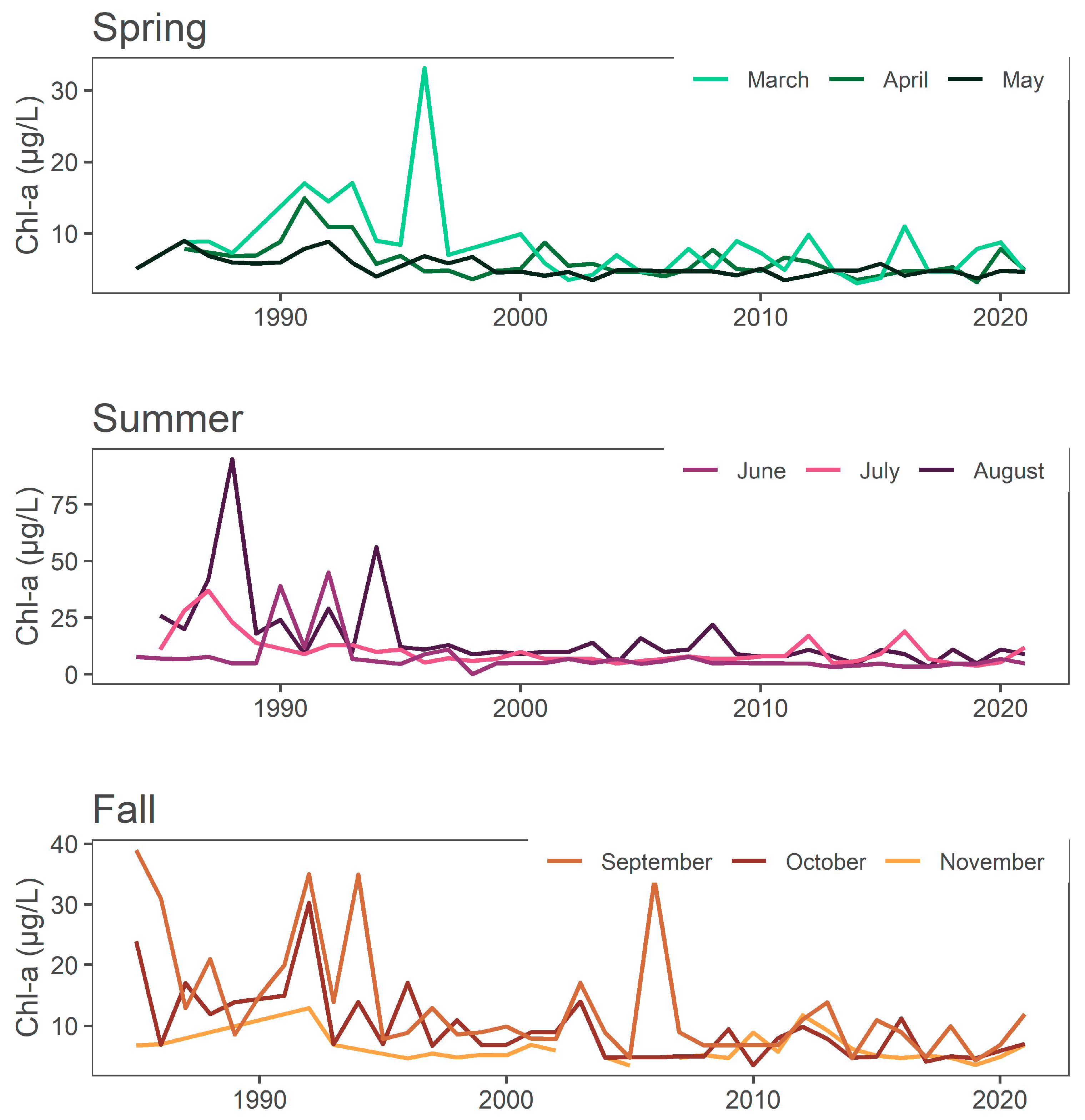
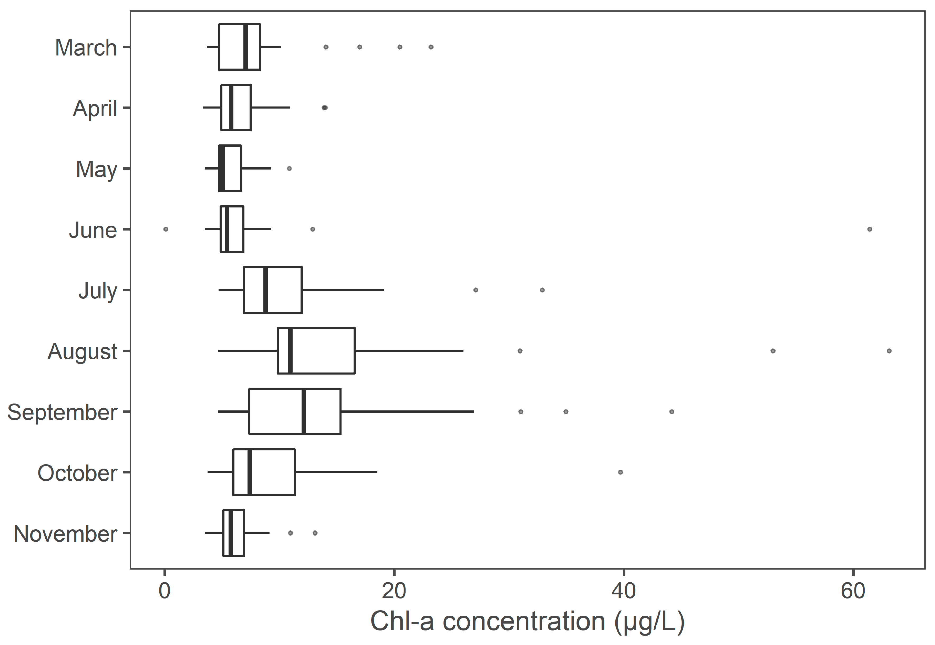
3.5. Monthly and Seasonal Chl-a Concentrations Regional Trends

To evaluate different temporal behaviors, we computed and plotted median values for each month, e.g., median values for April in 1984, April in 1985, April in 1986, etc. Figure 15 presents data similar to Figure 14, but as a time series with the individual months plotted separately. These plots show the impact of having higher frequency data after the launch of Landsat 7 in 1999. Prior to 1999, our dataset includes only images collected by Landsat 5, so one image every 16 days (or fewer if there was cloud cover). Landsat 7 is asynchronous with Landsat 5, so from 1999 onward there are images approximately every 8 days. In the earlier years of the dataset, there are many months with only a single usable image because of clouds, and if that image was collected on a day with an intense bloom or missed a bloom at another time in the month, it is not necessarily representative of conditions for that entire month and caused increased variability in the early portion of the data set. This means that the apparent high variability and higher values prior to 1999 are an artifact of the sampling period, and do not necessarily represent lake conditions.
The timing of algal blooms during the year appears not to have changed significantly over the study period—growth is lowest in the spring, peaks in the summer, then decreases slightly in the fall. Figure 15 illustrates how algal growth in Utah Lake cycles over time, with some years experiencing high concentrations during all 3 seasons, followed by years of low growth, with the pre-1990 data exhibiting large variability because of having a limited number of data points in a month. These cycles are most likely related to weather patterns and lake level variation during the study period. Figure 16 shows that chl-a trends for fall and summer appear to be more closely related than the trends for spring, indicating that algal growth in the spring is potentially influenced by different factors than algal growth in the summer and fall. This characteristic is more apparent in Figure 14, which summarizes the whole-lake median data into a single median value by season for each year in the study period. Both Figure 14 and Figure 16 show the predominantly lower values during spring and the high variability in chl-a concentrations during fall.
Figure 17 shows the distribution of whole-lake median values by month as data distributions, rather than time series and illustrates the typical yearly pattern of chl-a concentrations on Utah Lake. Median concentrations of chl-a during the summer and early fall were extremely variable over the study period, but consistently low during the spring and late fall. This is shown in both the change in the center of the distribution plot for each month and the increased variance shown by the box boundaries and outlier points.
Table 4 presents the M-K trend analysis of mean chl-a concentrations in Provo Bay. Most of the months have no significant trend. However, April, June, and December have a statistically significant increasing trends with p-values of 0.020, 0.000, and 0.002, respectively; 0.050 is considered significant. December only has 38 measurements, which means that trends must be more pronounced to be statistically significant. Overall Provo Bay has no trend, as determined by the M-K test (Table 3), but there are months with significant increasing trends.
In May, immediately after April, the estimated trend slope is decreasing, even though it is not statistically significant. July has increasing slopes, August immediately afterward has larger decreasing slopes, though neither are statistically significant. It is possible that the early season and mid-season blooms have started occurring earlier in the year towards the end of the ~40-year period, with April and June increasing, while the following months are decreasing. While this hypothesis is plausible, it is not convincingly supported by the data, though there are indications this could be occurring. The trend in January is decreasing, after the increasing trend in December which follows the same pattern.
Table 5 extends this analysis to all the lake regions. The majority of the analysis regions have a statistically significant decreasing trend for each of the non-winter months, Table 5 presents only the areas that do not have a decreasing trend for a particular month. Table 5 does not include Provo Bay results, as they were presented in Table 4. None of these areas have statistically significant trends and all the estimated slopes, except for Southern Lake in February, are decreasing or 0. However, the majority of the entries in this table are for the month of February, with the remainder mostly occurring in of March, April, May, or June, which indicates that these areas may be behaving slightly differently from the rest of the lake during these months. Although the anomalies are not pronounced enough to be significant over the 40-year period, they do show that these regions are behaving differently from the majority of the lake, which shows a statistically significant decrease. While the data are not conclusive, they do indicate the possibility that climate change is moving the early spring diatom bloom, the early green algal bloom, and the later blue-green algal bloom earlier into February, April, and July, respectively. The majority of these entries, when data from Table 4 is included, are for Provo Bay, the mouth of Provo Bay, or the southern end of the lake near Goshen Bay.
The only region with any months that exhibit increasing trends is Provo Bay with April, June, and December exhibiting increasing trends. The December data are questionable because of the time or the year. Except for Provo Bay in April and June, no other regions or months show increasing trends. Table 5 shows the regions and months that have no trends (mostly February which we again attribute to climate change).

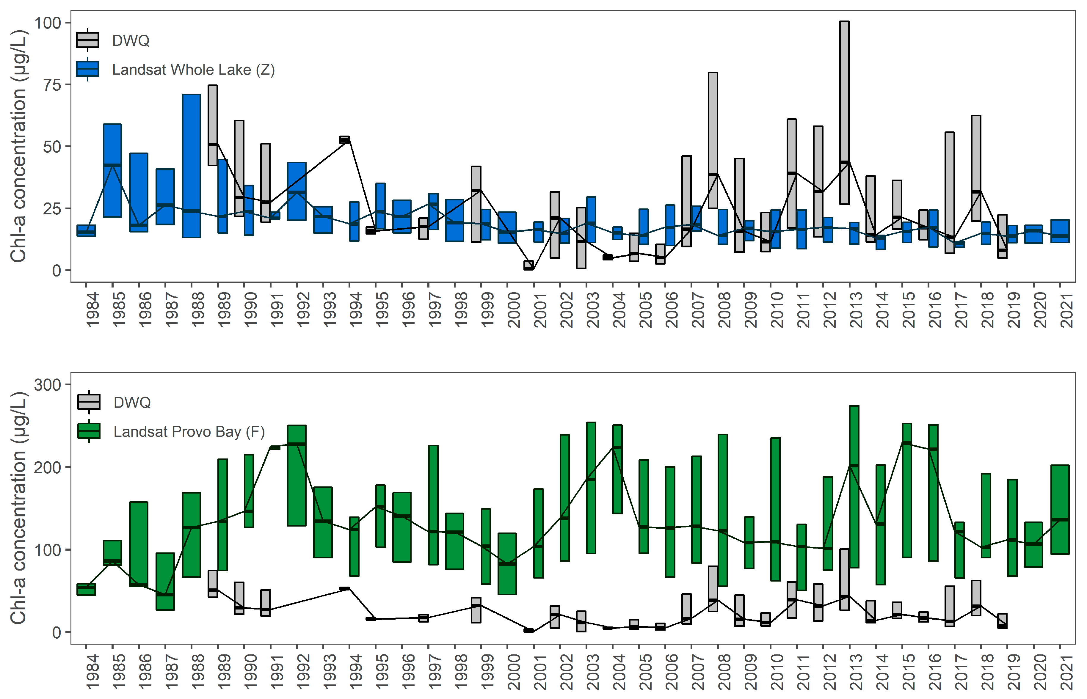
3.6. Comparison to Measured Data

To check the validity of the remotely-sensed chl-a estimates, we obtained chl-a data for Utah Lake from the Utah Department of Water Quality (DWQ) Ambient Water Quality Management System (AWQMS) database. The AWQMS data are taken at irregularly spaced locations (24 separate sampling points around the lake) with varying frequency. The most frequently sampled DWQ sampling location, just south of Provo Bay, was sampled 169 times over the 40-year study period. In contrast, the remote sensing estimates have around 650 data points per pixel over the study period. Many of the years in the study period do not have any AWQMS data.
Table 6 shows the 10 sampling locations with the most data. Locations near Provo Bay, Goshen Bay, and shoreline areas are over-represented in the AWQMS data. Lincoln Point and Lincoln Beach are on the eastern shore at the end of the narrow lake arm leading to Goshen Bay. Sampling locations inside or near Provo Bay are 4 of the top 10 most-frequently sampled locations. With Goshen Bay, Lincoln Point, and Lincoln Beach making up an additional 3 of the most-sampled points. The areas represented by these points have higher average chl-a concentrations (Figure 6) than the rest of the lake.
We compared both the annual distributions of the median values for the whole lake and the Provo Bay polygon to the annual distribution of the AWQMS data. We expected to AWQMS values to be generally higher than the whole lake Landsat estimates, since they were mainly collected in areas with higher chl-a concentrations, but lower than the Provo Bay estimates, as they are not limited to Provo Bay.
Figure 18 shows the annual distribution of the AQWMS data and the annual distributions of the median regional values for the whole lake and Provo Bay. Although the differences between the two datasets prevent this from being a rigorous comparison, Figure 18 shows that the Landsat estimates match the DWQ data fairly well, especially when the frequent sampling of high-chl-a areas is accounted for, and are a reasonable representation of chl-a concentrations in Utah Lake. DWQ values are nearly always higher than the whole lake values and lower than the Provo Bay values. This is more apparent after 2007, which we attribute to an increased focus of the data on Provo Bay. In 2001, 2004, and 2006, annual median AQWMS values were lower than the annual whole-lake average, but there were only a few AQWMS values for these years. We used a model from the literature [34] that was based on measured chl-a values below 100 ug/L. The current DWQ AQWMS data base included values over 300 ug/L, the limit we imposed on our estimates.
Tate [36] used a similar approach to ours, but evaluated only selected images based on cloud cover which with limited the number of images used for the study. Their results showed that the lake, in general had little to no trend over the last ~40 years, comparable to our findings. Their findings add support to our detailed analysis of individual lake regions, showing that our general findings are consistent with both in situ measured data from the DWQ AQWMS and previous remote sensing studies.

4. Discussion

Since the lake is extremely shallow for its size, with about 50% of its inflow lost to evaporation [54], spatial mixing within the lake is fairly limited. Because of this, we expected lake regions significantly impacted by shoreline development, WWTP effluent, and other nutrient inflows to show an increasing trend in chl-a concentrations, as the population around the lake has grown significantly over the study period. Such changes are not evident in the data. While there are differences in the average chl-a values for each region over the study period, the regions with higher values are mainly associated with Provo Bay.
The data show that chl-a concentrations in regions of the lake that have experienced development of the shoreline or receive effluent from WWTPs are not significantly different from those that have not. The center of the lake is also like the shoreline areas, with the exception of Provo Bay and the regions around Provo Bay.
Provo Bay does receive the outfalls from the Provo and Springville WWTPs, but these plants combined do not discharge as much effluent as TSSD, which discharges into Region B (North Shore) and is similar in size to the Orem WWTP, which discharges into Region C (NE Shore). While Provo Bay has significantly higher chl-a concentrations than other lake areas, there has been no significant changes in chl-a concentrations over the 40-year study period. While some areas of the bay have statistically significant increasing trends, the slope of these trends is minor, resulting in minimal changes, less than the variation in the data, over the study period.
While it is reasonable to assume that nutrient loadings increased with increased WWTP effluents, WWTPs have implemented additional and more efficient treatment processes over the 40-year period studied. In private discussions with WWTP operators, we were informed that WWTP effluent nutrient concentrations have decreased over time, even as total effluent volumes have increased, especially in the last 10 years. Because of this, although we expect that the WWTP nutrient load to the lake increased as the population of Utah County increased, the exact magnitude and timing of that increase is unknown.
We found no quantitative information on changes in nutrient fluxes due to shoreline development, but we assume that if development directly affected water quality in Utah Lake, it would be observable in the long-term data.
Our data support the hypothesis that, over the last 40 years, algal growth in Utah Lake has been limited by light availability in the water column and other factors and was not primarily driven by direct nutrient inflows. Previous studies have indicated that algal growth is light-limited at the high turbidity levels observed in Utah Lake [62]. Based on visual analysis of satellite images, Provo Bay has less turbid water. This lack of turbidity may allow more phytoplankton growth in the bay and, as water flows from Provo Bay into the lake, the regions surrounding the mouth of Provo Bay.

5. Conclusions

Our analysis of 40 years of remotely-sensed data on chl-a concentrations in Utah Lake showed that, for the lake as a whole, there has been essentially no change in algal growth since the 1980′s, despite significant population expansion and land-use changes in the lake’s watershed. Our data also showed that there is significant spatial and temporal variation in algal growth throughout the growing season. These results match previous remote-sensing studies on Utah Lake [36]. Further research is needed to better understand what specific factors might drive these changes. Although there is no trend for the lake as a whole, Provo Bay shows a slight increasing trend for certain pixels. The M-K test on data from the entire bay indicated there is no statistically significant trend over the 40-year study period. While some pixels in Provo Bay demonstrate increasing concentrations, the magnitude of these changes only results in increases of 4 and 0.2 µg/L over the study period, an insignificant amount given the average concentration is 132 µg/L, with monthly averages ranging from 18 to 200 µg/L for January and August, respectively. Monthly data do show increasing trends in chl-a concentrations in Provo Bay in April, June, and December. These data indicate that algal blooms in Provo Bay have not decreased as elsewhere in the lake and that, for some time periods, concentrations are increasing, offset by decreasing concentrations in other months. This could be driven by changing temperature patterns, moving peak algal growth to earlier in the year.
The Utah DWQ is considering various efforts to mitigate algal blooms in Provo Bay and Utah Lake as whole, many of which would be extremely costly and resource-intensive. Proposed actions include more restrictive guidelines on WWTPs and other nutrient sources. The justification for the high cost of implementing such restrictions depends on whether limiting nutrients from WWTPs and other controllable sources will significantly reduce algal growth on the lake. If in-lake nutrient levels are governed not by direct nutrient inflows but by in-lake geochemical processes, sediment sources, atmospheric deposition, and other natural non-point nutrient sources, as suggested by multiple researchers [19,20,63,64], then these restrictions on nutrient inflows may have limited impacts on algal blooms and other water quality issues compared to other mitigation strategies that more directly target the main drivers of blooms. Since direct nutrient inflows do not appear to be the main driver of algal blooms on Utah Lake over the last 40 years, a better understanding of the factors and processes influencing algal growth is necessary to determine the most effective strategies for improving and maintaining the health of Utah Lake.

Supplementary Materials

The following supporting information can be downloaded at: https://www.mdpi.com/article/10.3390/rs14153664/s1, This is a zipfile that contains maps of average chl-a concentrations for each month, and time series plots for each of the 17 study areas for both mean and median chl-a concentrations for the entire time period, by season, and by month.

Author Contributions

Conceptualization, G.P.W.; methodology, A.C.C. and G.P.W.; software, A.C.C. and G.P.W.; formal analysis, K.B.T., A.C.C. and G.P.W.; data curation, A.C.C. and K.B.T.; writing—original draft preparation, K.B.T., A.C.C. and G.P.W.; writing—review and editing, K.B.T., A.C.C. and G.P.W.; visualization, A.C.C. and K.B.T.; supervision, G.P.W.; project administration, G.P.W. All authors have read and agreed to the published version of the manuscript.

Funding

This research received no external funding.

Data Availability Statement

Publicly available datasets were analyzed in this study. This data can be found here https://developers.google.com/earth-engine/datasets.

Acknowledgments

We would like to thank A. Woodruff Miller, LaVere Merritt, David Richards, Jeff Den Bleyker, Richard Michelson, and Theron Miller, for their assistance and review of this study. We would like to thank the Utah Space Grant Fellowship for helping support students over the years in this field.

Conflicts of Interest

The authors declare no conflict of interest.

References

  1. Williams, G.P. Great Salt Lake and Utah Lake Statistical Analysis: Vol II: Utah Lake; Farmington Bay & Utah Lake Water Quality Council: Provo, UT, USA, 2020. [Google Scholar]
  2. Merritt, L.B.; Miller, A.W. Interim Report on Nutrient Loadings to Utah Lake: 2016; Jordan River, Farmington Bay & Utah Lake Water Quality Council: Provo, UT, USA, 2016. [Google Scholar]
  3. PSOMAS; SWCA. Utah Lake TMDL: Pollutant Loading Assessment & Designated Benificial Use Impairment Assessment—FINAL DRAFT; State of Utah Division of Water Quality: Salt Lake City, UT, USA, 2007; p. 88.
  4. UDWQ. Harmful Algal Blooms Home—Utah Department of Environmental Quality; Utah Divison of Water Quality: Salt Lake City, UT, USA, 2021. [Google Scholar]
  5. Alsanea, A. A Holistic Approach to Cyanobacterial Harmful Algal Blooms in Shallow, Eutrophic Utah Lake. Master of Science Dissertation, The University of Utah, Ann Arbor, MI, USA, 2018. [Google Scholar]
  6. Christoffersen, K. Ecological implications of cyanobacterial toxins in aquatic food webs. Phycologia 1996, 35, 42–50. [Google Scholar] [CrossRef]
  7. Sellner, K.G.; Doucette, G.J.; Kirkpatrick, G.J. Harmful algal blooms: Causes, impacts and detection. J. Ind. Microbiol. Biotechnol. 2003, 30, 383–406. [Google Scholar] [CrossRef] [PubMed]
  8. Carmichael, W.W. Health Effects of Toxin-Producing Cyanobacteria: “The CyanoHABs”. Hum. Ecol. Risk Assess. Int. J. 2001, 7, 1393–1407. [Google Scholar] [CrossRef]
  9. Johnston, B.R.; Jacoby, J.M. Cyanobacterial toxicity and migration in a mesotrophic lake in western Washington, USA. Hydrobiologia 2003, 495, 79–91. [Google Scholar] [CrossRef]
  10. Paerl, H.W.; Huisman, J. Climate change: A catalyst for global expansion of harmful cyanobacterial blooms. Environ. Microbiol. Rep. 2009, 1, 27–37. [Google Scholar] [CrossRef] [PubMed]
  11. Jöhnk, K.D.; Huisman, J.; Sharples, J.; Sommeijer, B.; Visser, P.M.; Stroom, J.M. Summer heatwaves promote blooms of harmful cyanobacteria. Glob. Change Biol. 2008, 14, 495–512. [Google Scholar] [CrossRef] [Green Version]
  12. Sharma, S.; Gray, D.K.; Read, J.S.; O’Reilly, C.M.; Schneider, P.; Qudrat, A.; Gries, C.; Stefanoff, S.; Hampton, S.E.; Hook, S.; et al. A global database of lake surface temperatures collected by in situ and satellite methods from 1985–2009. Sci. Data 2015, 2, 150008. [Google Scholar] [CrossRef] [Green Version]
  13. Straile, D. Meteorological forcing of plankton dynamics in a large and deep continental European lake. Oecologia 2000, 122, 44–50. [Google Scholar] [CrossRef] [Green Version]
  14. Paerl, H.W.; Paul, V.J. Climate change: Links to global expansion of harmful cyanobacteria. Water Res. 2012, 46, 1349–1363. [Google Scholar] [CrossRef]
  15. Anderson, D.M.; Glibert, P.M.; Burkholder, J.M. Harmful algal blooms and eutrophication: Nutrient sources, composition, and consequences. Estuaries 2002, 25, 704–726. [Google Scholar] [CrossRef]
  16. Strong, A.E. Remote sensing of algal blooms by aircraft and satellite in Lake Erie and Utah Lake. Remote Sens. Environ. 1974, 3, 99–107. [Google Scholar] [CrossRef]
  17. Merritt, L.B. Open Letter to the Utah Lake Science Panel & Lake Steering Committee; Utah Department of Environmental Quality: Salt Lake City, UT, USA, 2020; unpublished information.
  18. Dolder, D.; Williams, G.P.; Miller, A.W.; Nelson, E.J.; Jones, N.L.; Ames, D.P. Introducing an Open-Source Regional Water Quality Data Viewer Tool to Support Research Data Access. Hydrology 2021, 8, 91. [Google Scholar] [CrossRef]
  19. Olsen, J.; Williams, G.; Miller, A.; Merritt, L. Measuring and Calculating Current Atmospheric Phosphorous and Nitrogen Loadings to Utah Lake Using Field Samples and Geostatistical Analysis. Hydrology 2018, 5, 45. [Google Scholar] [CrossRef] [Green Version]
  20. Barrus, S.M.; Williams, G.P.; Miller, A.W.; Borup, M.B.; Merritt, L.B.; Richards, D.C.; Miller, T.G. Nutrient Atmospheric Deposition on Utah Lake: A Comparison of Sampling and Analytical Methods. Hydrology 2021, 8, 123. [Google Scholar] [CrossRef]
  21. Randall, M.C.; Carling, G.T.; Dastrup, D.B.; Miller, T.; Nelson, S.T.; Rey, K.A.; Hansen, N.C.; Bickmore, B.R.; Aanderud, Z.T. Sediment potentially controls in-lake phosphorus cycling and harmful cyanobacteria in shallow, eutrophic Utah Lake. PLoS ONE 2019, 14, e0212238. [Google Scholar] [CrossRef]
  22. UDWQ. Utah Lake Water Quality Work Plan 2015–2019; Utah Divison of Water Quality: Salt Lake City, UT, USA, 2016; p. 88.
  23. Kloiber, S.M.; Brezonik, P.L.; Olmanson, L.G.; Bauer, M.E. A procedure for regional lake water clarity assessment using Landsat multispectral data. Remote Sens. Environ. 2002, 82, 38–47. [Google Scholar] [CrossRef]
  24. Fuller, L.M.; Aichele, S.S.; Minnerick, R.J. Predicting Water Quality by Relating Secchi-Disk Transparency and Chlorophyll a Measurements to Satellite Imagery for Michigan Inland Lakes, August 2002; 2004–5086; US Geological Survey: Reston, VA, USA, 2004.
  25. Olmanson, L.G.; Bauer, M.E.; Brezonik, P.L. A 20-year Landsat water clarity census of Minnesota’s 10,000 lakes. Remote Sens. Environ. 2008, 112, 4086–4097. [Google Scholar] [CrossRef]
  26. Brezonik, P.; Menken, K.D.; Bauer, M. Landsat-based Remote Sensing of Lake Water Quality Characteristics, Including Chlorophyll and Colored Dissolved Organic Matter (CDOM). Lake Reserv. Manag. 2005, 21, 373–382. [Google Scholar] [CrossRef]
  27. Brivio, P.A.; Giardino, C.; Zilioli, E. Determination of chlorophyll concentration changes in Lake Garda using an image-based radiative transfer code for Landsat TM images. Int. J. Remote Sens. 2001, 22, 487–502. [Google Scholar] [CrossRef]
  28. Kutser, T. Quantitative detection of chlorophyll in cyanobacterial blooms by satellite remote sensing. Limnol. Oceanogr. 2004, 49, 2179–2189. [Google Scholar] [CrossRef]
  29. Ma, R.; Dai, J. Investigation of chlorophyll-a and total suspended matter concentrations using Landsat ETM and field spectral measurement in Taihu Lake, China. Int. J. Remote Sens. 2005, 26, 2779–2795. [Google Scholar] [CrossRef]
  30. Mayo, M.; Gitelson, A.; Yacobi, Y.; Ben-Avraham, Z. Chlorophyll distribution in lake Kinneret determined from Landsat Thematic Mapper data. Remote Sens. 1995, 16, 175–182. [Google Scholar] [CrossRef]
  31. Yip, H.; Johansson, J.; Hudson, J. A 29-year assessment of the water clarity and chlorophyll-a concentration of a large reservoir: Investigating spatial and temporal changes using Landsat imagery. J. Great Lakes Res. 2015, 41, 34–44. [Google Scholar] [CrossRef]
  32. Allan, M.G.; Hamilton, D.P.; Hicks, B.; Brabyn, L. Empirical and semi-analytical chlorophyll a algorithms for multi-temporal monitoring of New Zealand lakes using Landsat. Environ. Monit. Assess. 2015, 187, 1–24. [Google Scholar] [CrossRef] [PubMed]
  33. NASA. Landsat—Earth Observation Satellites; 2015–3081; National Aeronautics and Space Administration: Reston, VA, USA, 2016; p. 4. [Google Scholar]
  34. Hansen, C.H.; Burian, S.J.; Dennison, P.E.; Williams, G.P. Evaluating historical trends and influences of meteorological and seasonal climate conditions on lake chlorophyll a using remote sensing. Lake Reserv. Manag. 2020, 36, 45–63. [Google Scholar] [CrossRef]
  35. Hansen, C.H.; Williams, G.P.; Adjei, Z. Long-term application of remote sensing chlorophyll detection models: Jordanelle Reservoir case study. Nat. Resour. 2015, 6, 123–129. [Google Scholar] [CrossRef] [Green Version]
  36. Tate, R.S. Landsat Collections Reveal Long-Term Algal Bloom Hot Spots of Utah Lake. Master’s Thesis, Brigham Young University, Provo, UT, USA, 2019. [Google Scholar]
  37. Le, C.; Li, Y.; Zha, Y.; Wang, Q.; Zhang, H.; Yin, B. Remote sensing of phycocyanin pigment in highly turbid inland waters in Lake Taihu, China. Int. J. Remote Sens. 2011, 32, 8253–8269. [Google Scholar] [CrossRef]
  38. Gons, H.J. Optical Teledetection of Chlorophyllain Turbid Inland Waters. Environ. Sci. Technol. 1999, 33, 1127–1132. [Google Scholar] [CrossRef]
  39. Nelson, S.A.C.; Soranno, P.A.; Cheruvelil, K.S.; Batzli, S.A.; Skole, D.L. Regional assessment of lake water clarity using satellite remote sensing. J. Limnol. 2003, 62, 27. [Google Scholar] [CrossRef] [Green Version]
  40. Bertani, I.; Steger, C.E.; Obenour, D.R.; Fahnenstiel, G.L.; Bridgeman, T.B.; Johengen, T.H.; Sayers, M.J.; Shuchman, R.A.; Scavia, D. Tracking cyanobacteria blooms: Do different monitoring approaches tell the same story? Sci. Total Environ. 2017, 575, 294–308. [Google Scholar] [CrossRef] [Green Version]
  41. Augusto-Silva, P.; Ogashawara, I.; Barbosa, C.; De Carvalho, L.; Jorge, D.; Fornari, C.; Stech, J. Analysis of MERIS Reflectance Algorithms for Estimating Chlorophyll-a Concentration in a Brazilian Reservoir. Remote Sens. 2014, 6, 11689–11707. [Google Scholar] [CrossRef] [Green Version]
  42. Cox, R.M.; Forsythe, R.D.; Vaughan, G.E.; Olmsted, L.L. Assessing Water Quality in Catawba River Reservoirs Using Landsat Thematic Mapper Satellite Data. Lake Reserv. Manag. 1998, 14, 405–416. [Google Scholar] [CrossRef]
  43. Ho, J.C.; Michalak, A.M. Challenges in tracking harmful algal blooms: A synthesis of evidence from Lake Erie. J. Great Lakes Res. 2015, 41, 317–325. [Google Scholar] [CrossRef] [Green Version]
  44. Shi, K.; Zhang, Y.; Qin, B.; Zhou, B. Remote sensing of cyanobacterial blooms in inland waters: Present knowledge and future challenges. Sci. Bull. 2019, 64, 1540–1556. [Google Scholar] [CrossRef] [Green Version]
  45. Bureau, U.S.C. Annual Estimates of the Resident Population: 1 April 2010 To 1 July 2019. Available online: https://data.census.gov/cedsci/table?q=Utah%20County,%20Utah%20Populations%20and%20People&tid=PEPPOP2019.PEPANNRES (accessed on 29 October 2021).
  46. Bureau, U.S.C. US Census Bureau Publications-Census of Population and Housing. Available online: https://www.census.gov/prod/www/decennial.html (accessed on 29 October 2021).
  47. Call, E. Calculating the Impact of ~65 years of Anthropogenic Activity on the Utah Lake Watershed Using Remote Sensing and Spatial Modeling. 2019. Available online: https://digitalcommons.usu.edu/runoff/2019/all/21/ (accessed on 29 October 2021).
  48. Hansen, C. Google Earth Engine as a Platform for Making Remote Sensing of Water Resources a Reality for Monitoring Inland Waters. 2015. Available online: https://www.researchgate.net/profile/Carly-Hansen-2/research (accessed on 29 October 2021).
  49. Cardall, A.; Tanner, K.B.; Williams, G.P. Google Earth Engine Tools for Long-Term Spatiotemporal Monitoring of Chlorophyll-a Concentrations. Open Water J. 2021, 7, 4. [Google Scholar]
  50. Masek, J.G.; Vermote, E.F.; Saleous, N.E.; Wolfe, R.; Hall, F.G.; Huemmrich, K.F.; Feng, G.; Kutler, J.; Teng-Kui, L. A Landsat surface reflectance dataset for North America, 1990–2000. IEEE Geosci. Remote Sens. Lett. 2006, 3, 68–72. [Google Scholar] [CrossRef]
  51. Vermote, E.; Justice, C.; Claverie, M.; Franch, B. Preliminary analysis of the performance of the Landsat 8/OLI land surface reflectance product. Remote Sens. Environ. 2016, 185, 46–56. [Google Scholar] [CrossRef] [PubMed]
  52. Hansen, C.H.; Williams, G.P. Evaluating Remote Sensing Model Specification Methods for Estimating Water Quality in Optically Diverse Lakes throughout the Growing Season. Hydrology 2018, 5, 62. [Google Scholar] [CrossRef] [Green Version]
  53. Xu, H. A study on information extraction of water body with the modified normalized difference water index (MNDWI). J. Remote Sens. 2005, 5, 589–595. [Google Scholar]
  54. Fuhriman, D.K.; Merritt, L.B.; Miller, A.W.; Stock, H.S. Hydrology and water quality of Utah Lake. Great Basin Nat. Mem. 1981, 5, 43–67. [Google Scholar]
  55. Mann, H.B. Nonparametric Tests Against Trend. Econometrica 1945, 13, 245. [Google Scholar] [CrossRef]
  56. Meals, D.W.; Spooner, J.; Dressing, S.A.; Harcum, J.B. Statistical Analysis for Monotonic Trends; US EPA: National Nonpoint Source Monitoring Program: Tech Notes 6; Tetra Tech, Inc.: Fairfax, VA, USA, 2011. [Google Scholar]
  57. Gilbert, R.O. Statistical Methods for Environmental Pollution Monitoring; John Wiley & Sons: New York, NY, USA, 1987. [Google Scholar]
  58. Helsel, D.R.; Hirsch, R.M. Statistical Methods in Water Resources, 1st ed.; Elsevier: Amsterdam, The Netherlands, 1992; Volume 49. [Google Scholar]
  59. Anaconda.org. Conda-Forge/Packages/Pymannkendall 1.4.2. Available online: https://anaconda.org/conda-forge/pymannkendall (accessed on 1 August 2021).
  60. Harris, C.R.; Millman, K.J.; van der Walt, S.J.; Gommers, R.; Virtanen, P.; Cournapeau, D.; Wieser, E.; Taylor, J.; Berg, S.; Smith, N.J.; et al. Array programming with NumPy. Nature 2020, 585, 357–362. [Google Scholar] [CrossRef] [PubMed]
  61. Helsel, D.R.; Hirsch, R.M.; Ryberg, K.R.; Archfield, S.A.; Gilroy, E.J. Statistical Methods in Water Resources; 4-A3; United States Geological Survey (USGS): Reston, VA, USA, 2020; p. 484.
  62. Jones, J. Experimental evidence of light and nutrient limitation of algal growth in a turbid midwest reservoir. Arch. Fur Hydrobiol. 1996, 135, 321–335. [Google Scholar]
  63. Abu-Hmeidan, H.Y.; Williams, G.P.; Miller, A.W. Characterizing total phosphorus in current and geologic utah lake sediments: Implications for water quality management issues. Hydrology 2018, 5, 8. [Google Scholar] [CrossRef] [Green Version]
  64. Casbeer, W.; Williams, G.P.; Borup, M.B. Phosphorus distribution in delta sediments: A unique data set from deer creek reservoir. Hydrology 2018, 5, 58. [Google Scholar] [CrossRef] [Green Version]
Figure 1. Example image from 24 September 1988 showing the issue with out-of-band pixels on the chl-a model. The left panel is a visual image, the center panel shows chl-a data with values over 300 µg/L clipped, and the right panel shows the image with the values over 300 µg/L set to 300 µg/L.
Remotesensing 14 03664 g001
Figure 2. Process flow chart from Cardall et al. [49].
Remotesensing 14 03664 g002
Figure 3. An example showing the different types of masks with chl-a concentration images from 11 April 2012 and 1 August 2012 for the left and right panels, respectively. The background map shows the approximate area of Utah Lake in blue, masked pixels are transparent, and pixels not masked are pale yellow to dark green based on chl-a concentrations. The left panel shows areas that are masked to eliminate cloud-contaminated pixels and pixels that are impacted by scan-line errors. The right panel shows pixels masked by whether or not the pixel contains land. On this date, the lake level was very low and both Provo Bay and Goshen Bay had significant exposed shoreline.
Remotesensing 14 03664 g003
Figure 4. The left panel of this figure shows the number of pixels used in computing the mean, median, and standard deviation, and other summary statistics. The right panel shows details of some features demonstrating how water level changes impact the number of pixels over the long-term period.
Remotesensing 14 03664 g004
Figure 5. Utah Lake statistical analysis regions. The smaller regions are shown in the left panel (regions A through P) and a lake center region is shown in the right panel (region Q). We also computed statistics for the entire lake.
Remotesensing 14 03664 g005
Figure 6. Mean (left) and median (right) average chl-a concentrations over the ~40-year study period. A non-linear color scale was selected to highlight lower concentration ranges in order to show the differences in the middle lake area, since concentrations outside of the two shallow bays are comparatively low.
Remotesensing 14 03664 g006
Figure 7. The standard deviation of chl-a concentration over the study period. Areas with the highest concentrations and those most impacted by water level changes have the highest standard deviation.
Remotesensing 14 03664 g007
Figure 8. Example chl-a distributions in panels (A,B) for a Lake-wide bloom and a bloom on the eastern shore on for 22 July 1988 and 24 September 1988, respectively. Panels (C,D) show blooms developing in Provo Bay over an approximate two-week period on 31 August 2014, and 16 September 2014, 16 days later and show the bloom moving from Provo Bay into the Lake and up along the eastern shore. Panels (E,F) show blooms developing in Provo Bay and Goshen Bay on 3 September and two weeks later on 19 September 2021 which appears to show water with high chl-a concentrations flowing out from the large blooms in the two bays into the lake.
Remotesensing 14 03664 g008
Figure 9. A map showing whether chl-a concentration trends are increasing or decreasing (left panel), areas with no trend are blank (white), while the right panel shows if the trends are statistically significant.
Remotesensing 14 03664 g009
Figure 10. A map showing the distribution of p-values. Areas in maroon, yellow, and purple indicate that there is less than 1%, less than 5%, or more than 5% chance, respectively, that the computed trend is due to random processes. We selected p-value of 0.05 (5%) as the significance level.
Remotesensing 14 03664 g010
Figure 11. Maps showing the slope of the chl-a trend computed for individual pixels using Sen’s Slope method (left panel) and a fitted linear regression line (right panel).
Remotesensing 14 03664 g011
Figure 12. Median chl-a values from March through November for selected analysis regions.
Remotesensing 14 03664 g012
Figure 13. Seasonal median chl-a values by location.
Remotesensing 14 03664 g013
Figure 14. Box-and-whisker plots showing the seasonal variation of the distribution of median chl-a values for the entire lake over the 40-year study period. Outliers above 25 µg/L excluded.
Remotesensing 14 03664 g014
Figure 15. Time history of median chl-a by month and season for the study period. Note that the y-axes are not identical for each season.
Remotesensing 14 03664 g015
Figure 16. Time series of median values for the whole lake by season.
Remotesensing 14 03664 g016
Figure 17. Distribution of whole-lake median values by month.
Remotesensing 14 03664 g017
Figure 18. Comparison of Landsat chl-a estimates with DWQ data on chl-a in Utah Lake for our lake median (top panel) and Provo Bay median (bottom panel) with different scales. Our median lake data generally agree with the DWQ data, with DWQ being slightly higher because it is weighted towards locations with high chl-a content. The DWQ data lie between the median for the lake and Provo Bay, which we attribute to DWQ sample locations.
Remotesensing 14 03664 g018
Table 1. Band designations relevant to this study, varying by satellite [50].
Band Designations Satellite Bands
Band NameVariable NameLandsat 8Landsat 7Landsat 5
Blueb1211
Greenb2322
Redb3433
SWIR 1 1b5655
SWIR 1 2b7777
TIR 2b81066
1 shortwave infrared (SWIR). 2 thermal infrared (TIR).
Table 2. Utah Lake Statistical Analysis regions. The letter designations are from Figure 3.
NameArea Major Inflows, Outflows and Notes
Jordan RiverAThis region contains the only outlet to Utah Lake, the Jordan River. Until recently, this region was ecologically dominated by native mollusks, in particular the mussel Anodonta sp. These species no longer exist in this region to regulate water quality.
North ShoreBThis region contains TSSD, the largest WWTP that discharges into Utah Lake. Approximately 30% of the total WWTP discharge into the lake occurs here. The region received the discharge from the Geneve Steel plant WWTP, including potential metal contamination, until recently. The treatment ponds still retain water and discharge into the lake. American Fork and Lindon Marinas are in this region. This region is rapidly industrializing.
North East ShoreCThis region receives the discharge from the Orem, UT WWTP, which is routed through Powell Slough. It has a few seeps and springs originating from the Wasatch Range, with Powell Slough being prominent. Some seeps and springs have been diverted and ecologically modified, others are near shore and submerged during higher lake levels. Development has impacted those further from shore, changing the discharge path. The shoreline was dominated by a climax Fremont Cottonwood ecosystem that altered the ecological integrity of the lake’s receiving water. Only remnants remain. During the period of this study, this region was mostly pastureland until approximately 5 years ago, when it began to be developed into housing. It is now one of the fastest growing suburb communities in the nation, potentially impacting water quality.
East Central ShoreDThis region contains the inlet for the Provo River, the main tributary to Utah Lake and the most important June Sucker spawning habitat on the lake. It also has the largest marina on the lake at Utah Lake State Park. This shore is mostly pastureland or agriculture. The Provo River delta is currently undergoing restoration, which will result in changes to the lake functioning in this area. This was started recently and could impact the last year or two of the study.
Provo Bay MouthEThis region receives inflow from Provo Bay, and the inflowing water has likely been ecologically altered by the residence time in the bay.
Provo BayFProvo Bay receives inflow from several tributaries including Hobble Creek. It also receives effluent from Provo and Springville WWTPs. The shore is wetlands or pastureland, and there are some small corrals for livestock. Provo Bay is ecologically dissimilar to other regions of the lake due to its shallowness and large inflows into a smaller volume, resulting in less turbid water than the lake as a whole.
Southeast ShoreGThis area receives water from several seeps, springs, and small creeks. It receives effluent from the Spanish Fork WWTP. The substrate in much of this area is mostly sand and sheltered from southern winds, allowing for the highest densities of macrophytes in the lake.
Southern LakeHThis is the southern portion of the lake. There are several seeps and groundwater discharge points. The shore is mostly pastureland with agriculture runoff. There are also some warm springs under the lake.
Goshen BayIThis is a very shallow bay—while it is wet, water is often only a few inches deep. It is surrounded by agricultural fields and orchards. Because of the shallow water, there is significant growth of aquatic vegetation in the bay, which can interfere with chl-a estimates.
Southwest ShoreJThere are no continuous discharges to this region. There may be seeps in the lake.
West Central ShoreKThere are no continuous discharges to this region. There may be seeps in the lake. This area has housing near the shore with development starting about 10–15 years ago
Northwest ShoreLThere are seeps and springs in this region. The area is developed with housing near the shore. Higher-density development started about 20 years ago and is rapidly expanding.
North Central MNorthern center portion of the lake
Mid-north CentralNMid-northern portion of the lake
Mid-CentralOMid-center portion of the lake
South CentralPSouth center portion of the lake that contain numerous warm springs under the lake
Central LakeQCenter portion of the lake. This region is ecologically much different than the other regions in the lake mostly because of light limitation and easily-disturbed fine substrate.
Table 3. Trend analysis results for data from the entire study period including winter months.
AreaArea NameTrendSig.Sen’s SlopeRegression SlopeAvg Chl-aN
LakeUtah lakedecreasingTRUE−0.26−0.4820.16939
AJordan RiverdecreasingTRUE−0.23−0.6116.91856
BNorth ShoredecreasingTRUE−0.28−0.7217.07886
CNortheast ShoredecreasingTRUE−0.31−0.8120.31882
DEast Central ShoredecreasingTRUE−0.21−0.3217.84882
EProvo Bay MouthdecreasingTRUE−0.23−0.2923.51851
FProvo Bayno trendFALSE0.280.36132.10884
GSoutheast ShoredecreasingTRUE−0.33−0.5823.21871
HSouthern LakedecreasingTRUE−0.15−0.6618.95897
IGoshen BaydecreasingTRUE−0.78−1.1466.68892
JSouthwest ShoredecreasingTRUE−0.11−0.5213.62884
KWest Central ShoredecreasingTRUE−0.11−0.3411.99883
LNorthwest ShoredecreasingTRUE−0.10−0.2610.39872
MNorth CentraldecreasingTRUE−0.10−0.278.44893
NMid-north CentraldecreasingTRUE−0.08−0.177.94905
OMid-CentraldecreasingTRUE−0.07−0.177.99889
PSouth CentraldecreasingTRUE−0.08−0.239.16893
QCentral LakedecreasingTRUE−0.09−0.218.26928
Table 4. Monthly trend analysis for mean chl-a results for Provo Bay excluding winter months.
AreaMonthMedian Value
(Avg Chl-a)
TrendSig.pSen’s SlopeRegress. SlopeN
Provo Bay118.96no trendFALSE0.497−0.20−1.0438
Provo Bay224.30no trendFALSE0.0990.931.4147
Provo Bay356.53no trendFALSE0.3100.550.3861
Provo Bay477.95increasingTRUE0.0260.880.6565
Provo Bay595.18no trendFALSE0.348−0.41−0.4491
Provo Bay6134.33increasingTRUE0.0002.432.6091
Provo Bay7199.65no trendFALSE0.6650.270.01102
Provo Bay8206.42no trendFALSE0.605−0.32−0.12107
Provo Bay9179.38no trendFALSE0.3410.760.9593
Provo Bay10131.07no trendFALSE0.0531.431.6991
Provo Bay1189.44no trendFALSE0.1091.191.6160
Provo Bay1242.26increasingTRUE0.0021.291.9338
Table 5. Monthly trend analysis results for analysis areas without decreasing trends (excluding winter months and Provo Bay) sorted by p-value.
AreaMonthMedian
Chl-a (µg/L)
TrendSig.pSen’s SlopeRegress SlopeN
Mid-north Central24.46no trendFALSE0.9930.00−0.0148
Southern Lake24.74no trendFALSE0.6250.010.0148
Southeast Shore25.25no trendFALSE0.538−0.02−0.0745
West Central Shore24.54no trendFALSE0.363−0.04−0.0845
Northwest Shore24.77no trendFALSE0.440−0.04−0.0845
Central Lake24.36no trendFALSE0.698−0.01−0.0149
South Central24.27no trendFALSE0.733−0.01−0.0146
North Central24.61no trendFALSE0.119−0.07−0.0447
Provo Bay Mouth25.52no trendFALSE1.0000.000.0145
East Central Shore25.50no trendFALSE0.417−0.050.6945
Mid-Central24.11no trendFALSE0.609−0.02−0.0146
Goshen Bay26.85no trendFALSE0.405−0.02−0.0746
North Shore24.88no trendFALSE0.075−0.09−0.1146
Southwest Shore24.46no trendFALSE0.452−0.03−0.0747
Utah Lake (whole)24.80no trendFALSE0.8430.00−0.0349
Jordan River25.05no trendFALSE0.112−0.09−0.0143
North East Shore25.11no trendFALSE0.853−0.010.2345
Southern Lake45.51no trendFALSE0.090−0.04−0.0766
Southeast Shore47.03no trendFALSE0.357−0.03−0.1564
South Central45.01no trendFALSE0.096−0.04−0.0269
Provo Bay Mouth47.52no trendFALSE0.254−0.02−0.0566
Southwest Shore45.20no trendFALSE0.114−0.03−0.0365
Provo Bay Mouth58.70no trendFALSE0.087−0.07−0.2281
Provo Bay Mouth68.82no trendFALSE0.067−0.05−0.0789
Southeast Shore79.00no trendFALSE0.170−0.06−0.1999
Provo Bay Mouth710.85no trendFALSE0.344−0.020.0796
East Central Shore79.71no trendFALSE0.071−0.08−0.09102
Provo Bay Mouth814.89no trendFALSE0.095−0.16−0.32106
Provo Bay Mouth1010.78no trendFALSE0.286−0.04−0.0790
Table 6. The ten most sampled locations and number of chl-a samples from the DEQ AWQMS data base.
LocationCount
3 mi WNW of Lincoln Beach169
1 mi East of Pelican Point168
1 mi West of Provo Boat Harbor162
Outside entrance to Provo Bay158
Goshen Bay SW End117
Middle of Provo Bay116
1 mi NE of Lincoln Point83
0.5 mi W of Geneva Discharge68
1 mi SE of Bird Island68
2 mi W of Vineyard68
Publisher’s Note: MDPI stays neutral with regard to jurisdictional claims in published maps and institutional affiliations.

