
UAV-LiDAR Measurement of Vegetation Canopy Structure Parameters and Their Impact on Land–Air Exchange Simulation Based on Noah-MP Model

 , , , , , and
Abstract
:1. Introduction
2. Materials and Methods
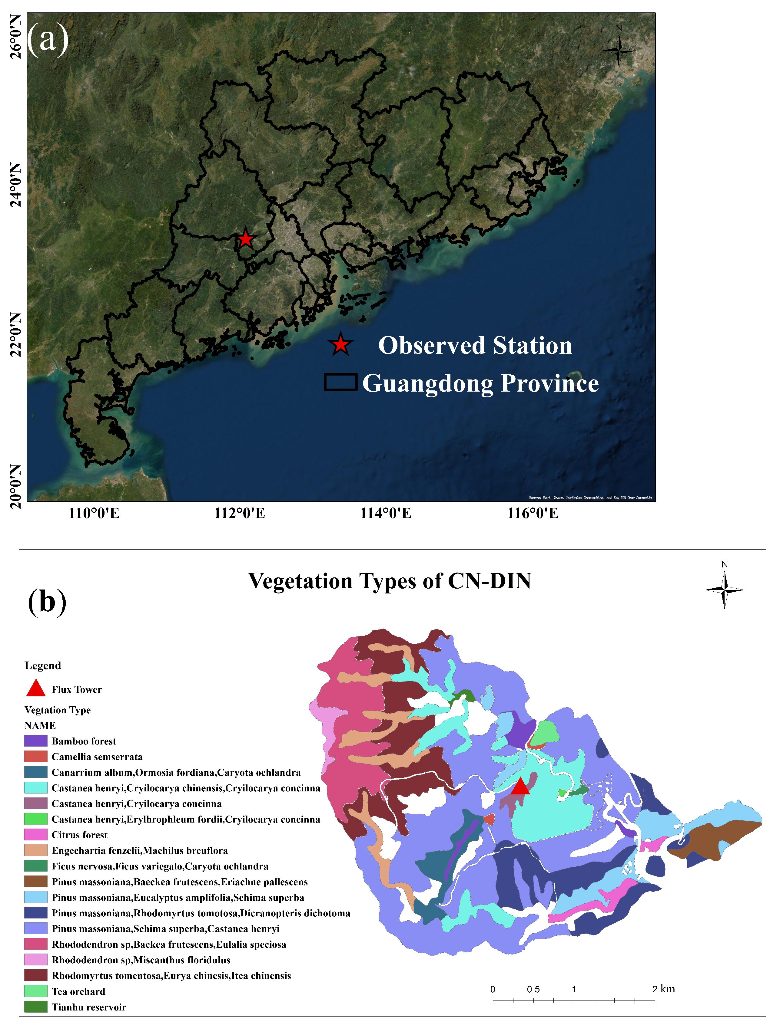
2.1. Study Area
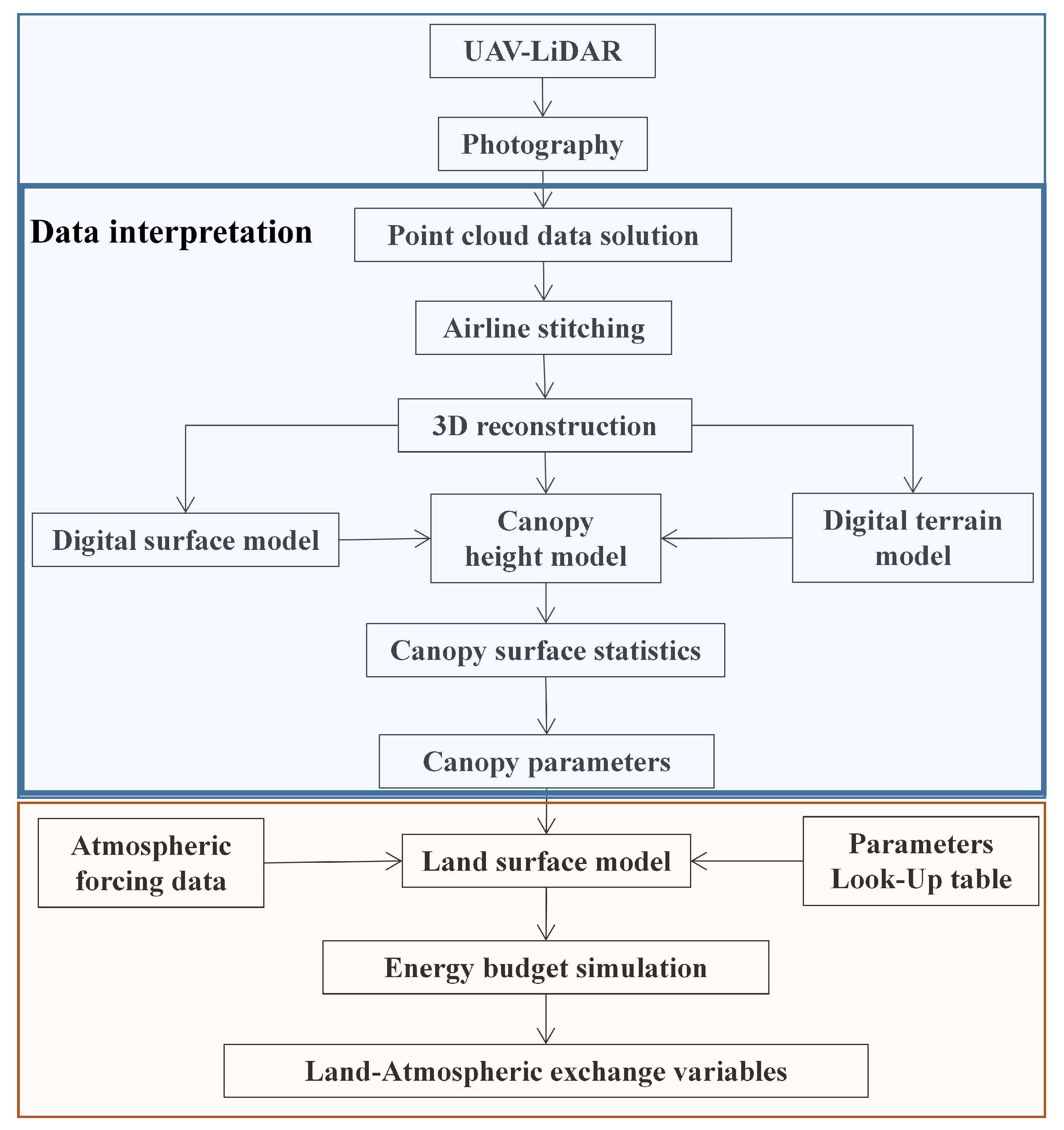
2.2. Workflow
2.3. Image Acquisition and Data Interpretation
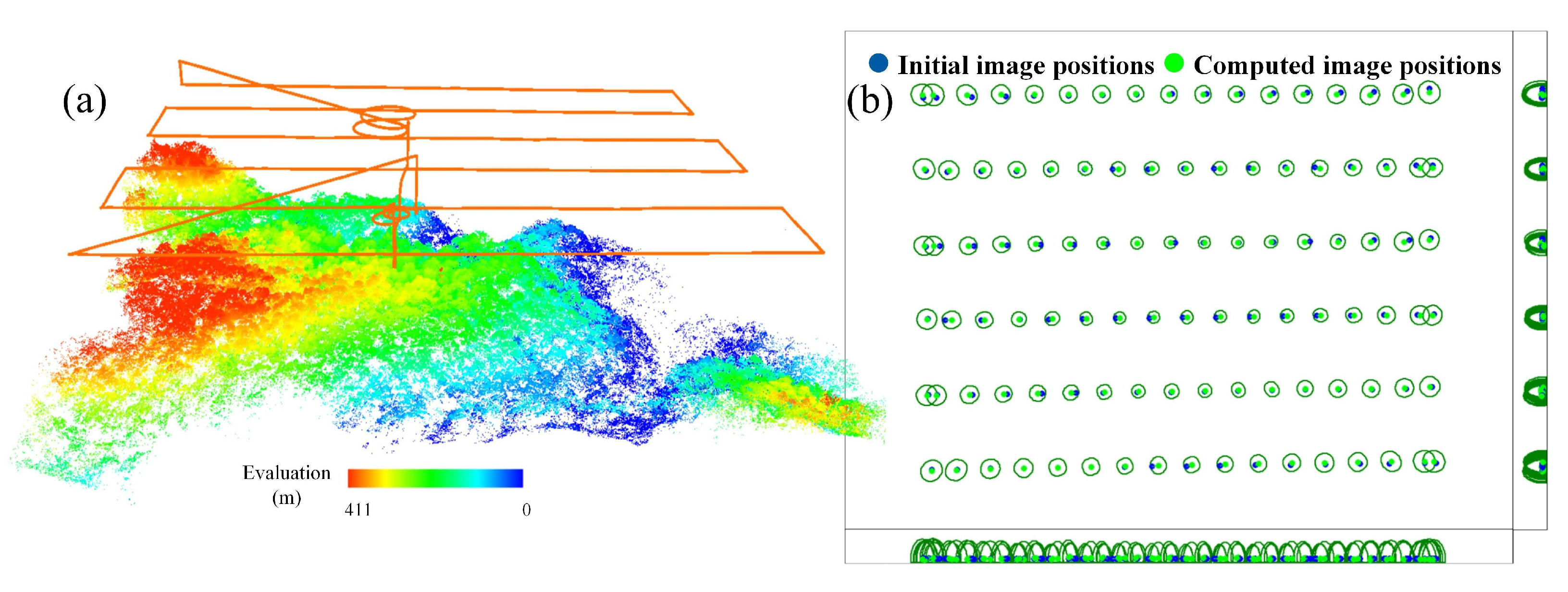
2.3.1. Photography
2.3.2. Data Interpretation
2.4. Land Surface Model Simulation
2.4.1. Atmospheric Forcing Data
2.4.2. Land Surface Model Setup And Validation
2.4.3. Vegetation Parameters Look-Up Table in Noah-MP
2.4.4. Energy Budget in Noah-MP
3. Results
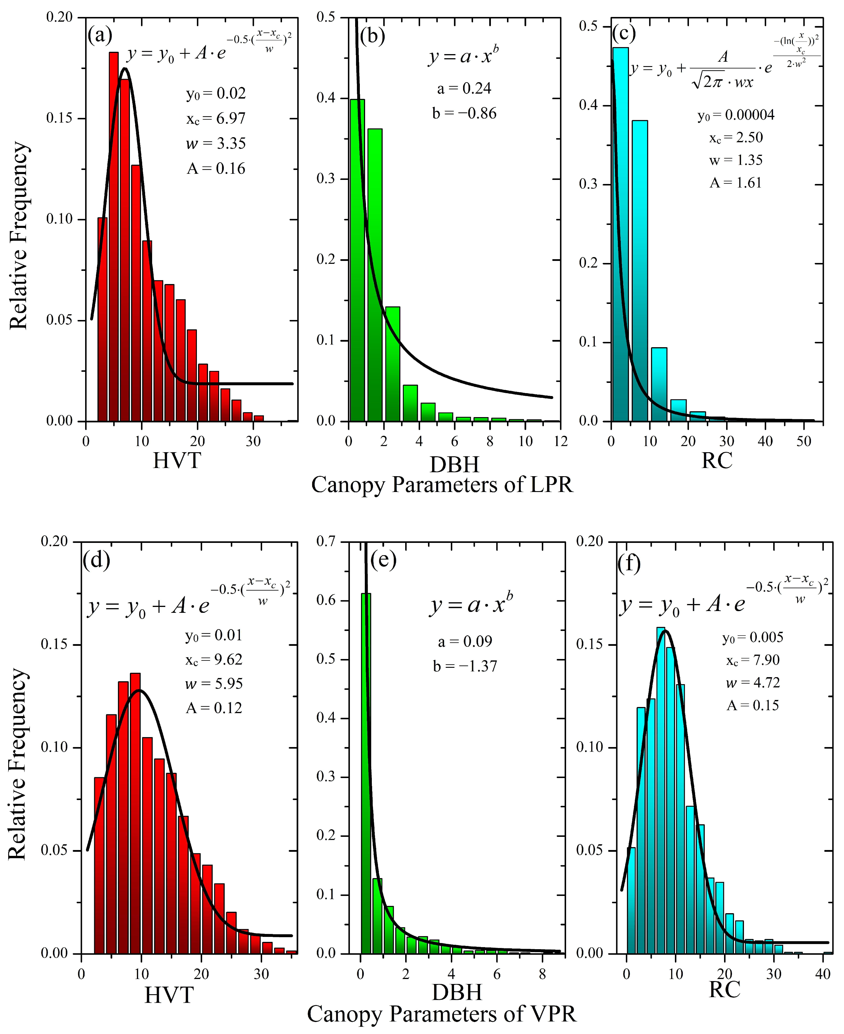
3.1. Characteristics of Measurement Results
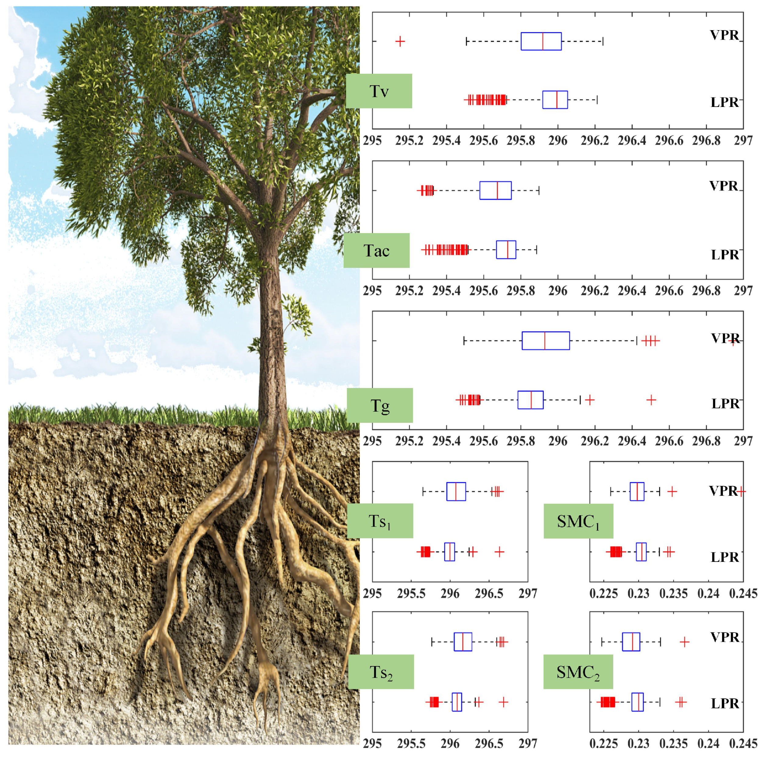
3.2. Results of the Simulated Canopy Temperature and Humidity Profiles
4. Discussion
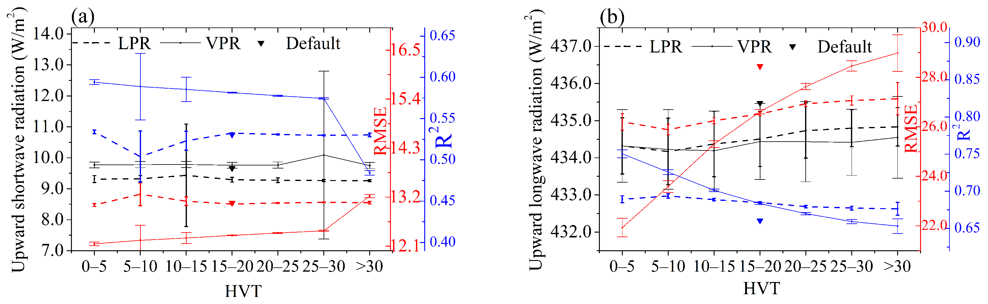
4.1. Diagnosis of the Upward Radiation Simulation
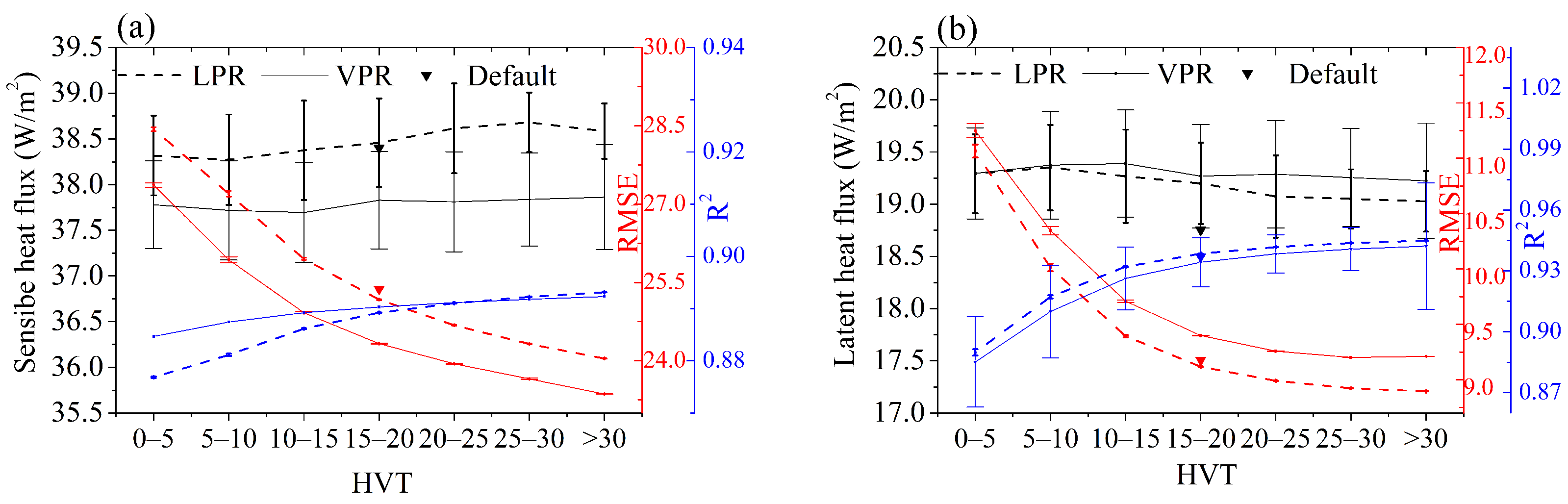
4.2. Diagnosis of the Surface Heat Flux Simulation
4.3. Limitations and Possible Improvements
5. Conclusions
Author Contributions
Funding
Data Availability Statement
Acknowledgments
Conflicts of Interest
Abbreviations
| Upward short-wave radiation | |
| Upward long-wave radiation | |
| Sensible heat flux | |
| Latent heat flux | |
| LPR | LiDAR photogrammetry results |
| VPR | Visible-light photogrammetry results |
| Tv | Vegetation temperature |
| Tac | Canopy air temperature |
| Tg | Ground temperature |
| Ts | Soil temperature |
| SMC | Soil moisture |
References
- Fang, Y.; Zou, X.; Lie, Z.; Xue, L. Variation in Organ Biomass with Changing Climate and Forest Characteristics across Chinese Forests. Forests 2018, 9, 521. [Google Scholar] [CrossRef] [Green Version]
- Pilotto, I.L.; Rodríguez, D.A.; Tomasella, J.; Sampaio, G.; Chou, S.C. Comparisons of the Noah-MP land surface model simulations with measurements of forest and crop sites in Amazonia. Meteorol. Atmos. Phys. 2015, 127, 711–723. [Google Scholar] [CrossRef]
- Zhang, X.; Chen, L.; Ma, Z.; Gao, Y. Assessment of surface exchange coefficients in the Noah-MP land surface model for different land-cover types in China. Int. J. Climatol. 2021, 41, 2638–2659. [Google Scholar] [CrossRef]
- Koster, R.D.; Suárez, M.J. Modeling the land surface boundary in climate models as a composite of independent vegetation stands. J. Geophys. Res. 1992, 97, 2697–2715. [Google Scholar] [CrossRef]
- Doran, J.; Zhong, S. Variations in mixed-layer depths arising from inhomogeneous surface conditions. J. Clim. 1995, 8, 1965–1973. [Google Scholar] [CrossRef] [Green Version]
- Lynch-Stieglitz, M. The Development and Validation of a Simple Snow Model for the GISS GCM. J. Clim. 1994, 7, 1842–1855. [Google Scholar] [CrossRef] [Green Version]
- Oki, T.; Sud, Y. Design of Total Runoff Integrating Pathways (TRIP)—A global river channel network. Earth Interact. 1998, 2, 1–37. [Google Scholar] [CrossRef]
- Kahan, D.S.; Xue, Y.; Allen, S.J. The impact of vegetation and soil parameters in simulations of surface energy and water balance in the semi-arid sahel: A case study using SEBEX and HAPEX-Sahel data. J. Hydrol. 2006, 320, 238–259. [Google Scholar] [CrossRef]
- Guo, Z.; Dirmeyer, P.A.; Hu, Z.; Gao, X.; Zhao, M. Evaluation of the Second Global Soil Wetness Project soil moisture simulations: 2. Sensitivity to external meteorological forcing. J. Geophys. Res. Atmos. 2006, 111, D22S03. [Google Scholar] [CrossRef] [Green Version]
- Veihe, A.; Quinton, J. Sensitivity analysis of EUROSEM using Monte Carlo simulation I: Hydrological, soil and vegetation parameters. Hydrol. Process. 2000, 14, 915–926. [Google Scholar] [CrossRef]
- Dai, Y.; Yuan, H.; Xin, Q.; Wang, D.; Shangguan, W.; Zhang, S.; Liu, S.; Wei, N. Different representations of canopy structure—A large source of uncertainty in global land surface modeling. Agric. For. Meteorol. 2019, 269–270, 119–135. [Google Scholar] [CrossRef]
- Webster, C.; Mazzotti, G.; Essery, R.; Jonas, T. Enhancing airborne LiDAR data for improved forest structure representation in shortwave transmission models. Remote Sens. Environ. 2020, 249, 15. [Google Scholar] [CrossRef]
- Paneque-Gálvez, J.; McCall, M.K.; Napoletano, B.M.; Wich, S.A.; Koh, L.P. Small Drones for Community-Based Forest Monitoring: An Assessment of Their Feasibility and Potential in Tropical Areas. Forests 2014, 5, 1481–1507. [Google Scholar] [CrossRef] [Green Version]
- Michałowska, M.; Rapiński, J. A Review of Tree Species Classification Based on Airborne LiDAR Data and Applied Classifiers. Remote Sens. 2021, 13, 353. [Google Scholar] [CrossRef]
- Guo, Q.; Su, Y.; Hu, T.; Guan, H.; Jin, S.; Zhang, J.; Zhao, X.; Xu, K.; Wei, D.; Kelly, M.; et al. Lidar Boosts 3D Ecological Observations and Modelings: A Review and Perspective. IEEE Geosci. Remote Sens. Mag. 2021, 9, 232–257. [Google Scholar] [CrossRef]
- Chang, M.; Zhu, S.J.; Cao, J.C.; Chen, B.Y.; Zhang, Q.; Chen, W.H.; Jia, S.G.; Krishnan, P.; Wang, X.M. Improvement and Impacts of Forest Canopy Parameters on Noah-MP Land Surface Model from UAV-Based Photogrammetry. Remote Sens. 2020, 12, 4120. [Google Scholar] [CrossRef]
- Reutebuch, S.E.; Andersen, H.E.; McGaughey, R.J. Light detection and ranging (LIDAR): An emerging tool for multiple resource inventory. J. For. 2005, 103, 286–292. [Google Scholar] [CrossRef]
- Korpela, I.; Ørka, H.O.; Maltamo, M.; Tokola, T.; Hyyppä, J. Tree species classification using airborne LiDAR–effects of stand and tree parameters, downsizing of training set, intensity normalization, and sensor type. Silva Fenn 2010, 44, 319–339. [Google Scholar] [CrossRef] [Green Version]
- Cao, L.; Coops, N.C.; Sun, Y.; Ruan, H.; Wang, G.; Dai, J.; She, G. Estimating canopy structure and biomass in bamboo forests using airborne LiDAR data. ISPRS J. Photogramm. Remote Sens. 2019, 148, 114–129. [Google Scholar] [CrossRef]
- Ferrarese, J.; Affleck, D.; Seielstad, C. Conifer crown profile models from terrestrial laser scanning. Silva Fenn 2015, 49, 1106. [Google Scholar] [CrossRef] [Green Version]
- Guan, H.; Su, Y.; Hu, T.; Wang, R.; Ma, Q.; Yang, Q.; Sun, X.; Li, Y.; Jin, S.; Zhang, J.; et al. A Novel Framework to Automatically Fuse Multiplatform LiDAR Data in Forest Environments Based on Tree Locations. IEEE Trans. Geosci. Remote Sens. 2020, 58, 2165–2177. [Google Scholar] [CrossRef]
- Guan, H.; Su, Y.; Sun, X.; Xu, G.; Li, W.; Ma, Q.; Wu, X.; Wu, J.; Liu, L.; Guo, Q. A marker-free method for registering multi-scan terrestrial laser scanning data in forest environments. ISPRS J. Photogramm. Remote Sens. 2020, 166, 82–94. [Google Scholar] [CrossRef]
- Hilker, T.; Coops, N.C.; Culvenor, D.S.; Newnham, G.; Wulder, M.A.; Bater, C.W.; Siggins, A. A simple technique for co-registration of terrestrial LiDAR observations for forestry applications. Remote Sens. Lett. 2012, 3, 239–247. [Google Scholar] [CrossRef]
- Liang, X.; Kukko, A.; Hyyppa, J.; Lehtomaki, M.; Pyorala, J.; Yu, X.; Kaartinen, H.; Jaakkola, A.; Wang, Y. In-situ measurements from mobile platforms: An emerging approach to address the old challenges associated with forest inventories. ISPRS J. Photogramm. Remote Sens. 2018, 143, 97–107. [Google Scholar] [CrossRef]
- Pierzchala, M.; Giguere, P.; Astrup, R. Mapping forests using an unmanned ground vehicle with 3D LiDAR and graph-SLAM. Comput. Electron. Agric. 2018, 145, 217–225. [Google Scholar] [CrossRef]
- Balsi, M.; Esposito, S.; Fallavollita, P.; Nardinocchi, C. Single-tree detection in high-density LiDAR data from UAV-based survey. Eur. J. Remote Sens. 2018, 51, 679–692. [Google Scholar] [CrossRef] [Green Version]
- Guo, Q.; Su, Y.; Hu, T.; Zhao, X.; Wu, F.; Li, Y.; Liu, J.; Chen, L.; Xu, G.; Lin, G.; et al. An integrated UAV-borne lidar system for 3D habitat mapping in three forest ecosystems across China. Int. J. Remote Sens. 2017, 38, 2954–2972. [Google Scholar] [CrossRef]
- Van der Zande, D.; Stuckens, J.; Verstraeten, W.W.; Mereu, S.; Muys, B.; Coppin, P. 3D modeling of light interception in heterogeneous forest canopies using ground-based LiDAR data. Int. J. Appl. Earth Obs. Geoinf. 2011, 13, 792–800. [Google Scholar] [CrossRef]
- Li, W.; Guo, Q.; Tao, S.; Su, Y. VBRT: A novel voxel-based radiative transfer model for heterogeneous three-dimensional forest scenes. Remote Sens. Environ. 2018, 206, 318–335. [Google Scholar] [CrossRef]
- Lamelas-Gracia, M.T.; Riaño, D.; Ustin, S. A LiDAR signature library simulated from 3-dimensional Discrete Anisotropic Radiative Transfer (DART) model to classify fuel types using spectral matching algorithms. GIScience Remote Sens. 2019, 56, 988–1023. [Google Scholar] [CrossRef]
- Regaieg, O.; Yin, T.; Malenovský, Z.; Cook, B.D.; Morton, D.C.; Gastellu-Etchegorry, J.P. Assessing impacts of canopy 3D structure on chlorophyll fluorescence radiance and radiative budget of deciduous forest stands using DART. Remote Sens. Environ. 2021, 265, 112673. [Google Scholar] [CrossRef]
- Braghiere, R.K.; Wang, Y.; Doughty, R.; Sousa, D.; Magney, T.; Widlowski, J.L.; Longo, M.; Bloom, A.A.; Worden, J.; Gentine, P.; et al. Accounting for canopy structure improves hyperspectral radiative transfer and sun-induced chlorophyll fluorescence representations in a new generation Earth System model. Remote Sens. Environ. 2021, 261, 112497. [Google Scholar] [CrossRef]
- Wang, Y.; Köhler, P.; He, L.; Doughty, R.; Braghiere, R.K.; Wood, J.D.; Frankenberg, C. Testing stomatal models at the stand level in deciduous angiosperm and evergreen gymnosperm forests using CliMA Land (v0.1). Geosci. Model Dev. 2021, 14, 6741–6763. [Google Scholar] [CrossRef]
- Liu, Q.; Fan, W.; Xu, B.; Zeng, Y.; Zhao, J. Regional Leaf Area Index Retrieval Based on Remote Sensing: The Role of Radiative Transfer Model Selection. Remote Sens. 2015, 7, 4604–4625. [Google Scholar] [CrossRef] [Green Version]
- Puliti, S.; Talbot, B.; Astrup, R. Tree-Stump Detection, Segmentation, Classification, and Measurement Using Unmanned Aerial Vehicle (UAV) Imagery. Forests 2018, 9, 102. [Google Scholar] [CrossRef] [Green Version]
- Ismail, Z.; Abdul Khanan, M.F.; Omar, F.; Abd Rahman, M.; Mohd Salleh, M.R. Evaluating Error of LiDar Derived DEM Interpolation for Vegetation Area. Int. Arch. Photogramm. Remote. Sens. Spat. Inf. Sci. 2016, XLII-4/W1, 141–150. [Google Scholar] [CrossRef] [Green Version]
- Zhou, Q.; Pilesjoe, P.; Chen, Y. Estimating surface flow paths on a digital elevation model using a triangular facet network. Water Resour. Res. 2011, 47, W07522. [Google Scholar] [CrossRef]
- Qi, C.; Baldocchi, D.; Gong, P.; Kelly, M. Isolating individual trees in a savanna woodland using small footprint lidar data. Photogramm. Eng. Remote Sens. 2006, 72, 923–932. [Google Scholar] [CrossRef] [Green Version]
- Chang, M.; Liao, W.; Wang, X.; Zhang, Q.; Chen, W.; Wu, Z.; Hu, Z. An optimal ensemble of the Noah-MP land surface model for simulating surface heat fluxes over a typical subtropical forest in South China. Agric. For. Meteorol. 2020, 281, 107815. [Google Scholar] [CrossRef]
- Niu, G.Y.; Yang, Z.L.; Mitchell, K.E.; Chen, F.; Ek, M.B.; Barlage, M.; Kumar, A.; Manning, K.; Niyogi, D.; Rosero, E.; et al. The community Noah land surface model with multiparameterization options (Noah-MP): 1. Model description and evaluation with local-scale measurements. J. Geophys. Res.-Atmos. 2011, 116, D12109. [Google Scholar] [CrossRef] [Green Version]
- Dickinson, R.E.; Shaikh, M.; Bryant, R.; Graumlich, L. Interactive Canopies for a Climate Model. J. Clim. 1998, 11, 2823–2836. [Google Scholar] [CrossRef]
- Ball, J.T.; Woodrow, I.E.; Berry, J.A. A model predicting stomatal conductance and its contribution to the control of photosynthesis under different environmental conditions. In Progress in Photosynthesis Research; Springer: Berlin/Heidelberg, Germany, 1987; pp. 221–224. [Google Scholar] [CrossRef]
- Chen, F.; Janjić, Z.; Mitchell, K. Impact of atmospheric surface-layer parameterizations in the new land-surface scheme of the NCEP mesoscale Eta model. Bound.-Layer Meteorol. 1997, 85, 391–421. [Google Scholar] [CrossRef]
- Niu, G.; Yang, Z. Effects of vegetation canopy processes on snow surface energy and mass balances. J. Geophys. Res. Atmos. 2004, 109, D23111. [Google Scholar] [CrossRef]
- Chen, F.; Mitchell, K.; Schaake, J.; Xue, Y.; Pan, H.; Koren, V.; Duan, Q.Y.; Ek, M.; Betts, A. Modeling of land surface evaporation by four schemes and comparison with FIFE observations. J. Geophys. Res. Atmos. 1996, 101, 7251–7268. [Google Scholar] [CrossRef] [Green Version]
- Niu, G.Y.; Yang, Z.L. Effects of frozen soil on snowmelt runoff and soil water storage at a continental scale. J. Hydrometeorol. 2006, 7, 937–952. [Google Scholar] [CrossRef]
- Barlage, M.; Tewari, M.; Chen, F.; Miguez-Macho, G.; Yang, Z.L.; Niu, G.Y. The effect of groundwater interaction in North American regional climate simulations with WRF/Noah-MP. Clim. Chang. 2015, 129, 485–498. [Google Scholar] [CrossRef]
- Niu, G.; Yang, Z.; Dickinson, R.E.; Gulden, L.E.; Su, H. Development of a simple groundwater model for use in climate models and evaluation with Gravity Recovery and Climate Experiment data. J. Geophys. Res. Atmos. 2007, 112, D07103. [Google Scholar] [CrossRef]
- Verseghy, D.L. CLASS—A Canadian land surface scheme for GCMs. I. Soil model. Int. J. Climatol. 1991, 11, 111–133. [Google Scholar] [CrossRef]
- Jordan, R.E. A one-dimensional temperature model for a snow cover: Technical documentation for SNTHERM. 89 US Army Corps Eng. 1991, 91–16, 49. [Google Scholar]
- Mendoza, P.A.; Clark, M.P.; Barlage, M.; Rajagopalan, B.; Samaniego, L.; Abramowitz, G.; Gupta, H. Are we unnecessarily constraining the agility of complex process-based models? Water Resour. Res. 2015, 51, 716–728. [Google Scholar] [CrossRef]
- Arsenault, K.R.; Nearing, G.S.; Wang, S.; Yatheendradas, S.; Peters-Lidard, C.D. Parameter Sensitivity of the Noah-MP Land Surface Model with Dynamic Vegetation. J. Hydrometeorol. 2018, 19, 815–830. [Google Scholar] [CrossRef]
- Yinglan, A.; Wang, G.Q.; Liu, T.X.; Shrestha, S.; Xue, B.L.; Tan, Z.X. Vertical variations of soil water and its controlling factors based on the structural equation model in a semi-arid grassland. Sci. Total Environ. 2019, 691, 1016–1026. [Google Scholar] [CrossRef] [PubMed]
- Fang, Y.; Mo, J.; Zhou, G.; Xue, J. Response of Diameter at Breast Height Increment to N Additions in Forests of Dinghushan Biosphere Reserve. J. Trop. Subtrop. Bot. 2005, 13, 198–204. [Google Scholar]
- Cheng, J.; Ouyang, X.; Huang, D.; Liu, S.; Zhang, D.; Li, Y. Sap flow characteristics of four dominant tree species in a mixed conifer-broadleaf forest in Dinghushan. Acta Ecol. Sin. 2015, 35, 4097–4104. [Google Scholar]
- Zhang, Q.; Han, R.; Zou, F. Effects of artificial afforestation and successional stage on a lowland forest bird community in southern China. For. Ecol. Manag. 2011, 261, 1738–1749. [Google Scholar] [CrossRef]
- Zou, S.; Geng, W.; Zhang, Q.; Zhou, G.; Liu, S.; Chu, G. A dataset of species composition in a monsoon evergreen broad- leaved forest monitoring plot of Dinghushan Forest Ecosystem Research Station (1992–2015). China Sci. Data 2019, 4, 1-7–7-7. [Google Scholar]
- Sui, D.; Wang, Y.; Lian, J.; Zhang, J.; Hu, J.; Ouyang, X.; Fan, Z.; Cao, H.; Ye, W. Gap distribution patterns in the south subtropical evergreen broad-leaved forest of Dinghushan. Biodiv. Sci. 2017, 25, 382–392. [Google Scholar] [CrossRef]
- Li, Y.; Mwangi, B.; Zhou, S.; Liu, S.; Zhang, Q.; Liu, J.; Chu, G.; Tang, X.; Zhang, D.; Wei, S.; et al. Effects of Typhoon Mangkhut on a Monsoon Evergreen Broad-Leaved Forest Community in Dinghushan Nature Reserve, Lower Subtropical China. Front. Ecol. Evol. 2021, 9, 692155. [Google Scholar] [CrossRef]
- Cho, E.; Choi, M. Regional scale spatio-temporal variability of soil moisture and its relationship with meteorological factors over the Korean peninsula. J. Hydrol. 2014, 516, 317–329. [Google Scholar] [CrossRef]
- Yang, Q.; Dan, L.; Lv, M.; Wu, J.; Li, W.; Dong, W. Quantitative assessment of the parameterization sensitivity of the Noah-MP land surface model with dynamic vegetation using ChinaFLUX data. Agric. For. Meteorol. 2021, 307, 108542. [Google Scholar] [CrossRef]
- Chen, F.; Zhang, Y. On the coupling strength between the land surface and the atmosphere: From viewpoint of surface exchange coefficients. Geophys. Res. Lett. 2009, 36, L10404. [Google Scholar] [CrossRef] [Green Version]
- Ruiz-Barradas, A.; Nigam, S. Warm season rainfall variability over the US great plains in observations, NCEP and ERA-40 reanalyses, and NCAR and NASA atmospheric model simulations. J. Clim. 2005, 18, 1808–1830. [Google Scholar] [CrossRef]
- Garcia, M.; Saatchi, S.; Ferraz, A.; Silva, C.A.; Ustin, S.; Koltunov, A.; Balzter, H. Impact of data model and point density on aboveground forest biomass estimation from airborne LiDAR. Carbon Balance Manag. 2017, 12, 4. [Google Scholar] [CrossRef] [PubMed] [Green Version]
- Chen, L.; Li, Y.; Chen, F.; Barlage, M.; Zhang, Z.; Li, Z. Using 4-km WRF CONUS simulations to assess impacts of the surface coupling strength on regional climate simulation. Clim. Dyn. 2019, 53, 6397–6416. [Google Scholar] [CrossRef]
- White, J.C.; Wulder, M.A.; Vastaranta, M.; Coops, N.C.; Pitt, D.; Woods, M. The Utility of Image-Based Point Clouds for Forest Inventory: A Comparison with Airborne Laser Scanning. Forests 2013, 4, 518–536. [Google Scholar] [CrossRef] [Green Version]
- Luo, D.; Lin, H.; Jin, Z.; Zheng, H.; Song, Y.; Feng, L.; Guo, Q. Applications of UAV digital aerial photogrammetry and LiDAR in geomorphology and land cover research. J. Earth Environ. 2019, 10, 213–226. [Google Scholar]


| Type of Land Surface Process | Physical Processes | Description | Options | Contents |
|---|---|---|---|---|
| Vegetation | OPT_DVEG | Mainly used to calculate leaf area index and vegetation cover. | 2 | Dynamic Vegatation Model [41] |
| OPT_CRS | Calculation of foliar stomatal impedance. Stomatal impedance influences the magnitude of the latent heat flux brought about by vegetation through leaf transpiration. | 1 | Ball–Berry Scheme [42] | |
| OPT_SFC | The calculation of the transport coefficient , which in the model reflects the strength of the energy exchange between land and air, is carried out. | 2 | Noah Type [43] | |
| OPT_RAD | Used to parametrically represent the canopy structure of the vegetation in the grid. | 1 | Gap = f (3D, cosz) [44] | |
| Soil | OPT_BTR | For the calculation of soil moisture, which can influence stomatal conductivity, photosynthesis, and soil decomposition. | 1 | Noah Type [45] |
| OPT_INF | Expresses the process of water infiltration in permafrost. | 1 | NY06 [46] | |
| OPT_TBOT | For the selection of boundary conditions of soil temperature. | 2 | Original Noah [47] | |
| OPT_STC | For the selection of snow/soil temperature time scenarios. | 1 | Semi-Implicit [40] | |
| Water | OPT_RUN | Used to simulate runoff, groundwater, and the changes in soil moisture they cause. | 1 | SIMGM [48] |
| OPT_FRZ | Used to calculate the amount of liquid and solid water in the soil when it freezes. | 1 | NY06 [46] | |
| OPT_ALB | Used to calculate the surface albedo of snow on the ground. | 2 | CLASS [49] | |
| OPT_SNF | Distinguishes between rainfall and snowfall. | 1 | Jordan [50] |
| Parameter Name | Description | Value | Units |
|---|---|---|---|
| Z0MVT | Momentum roughness length | 0.8 | m |
| HVT | Height of canopy | 16 | m |
| RC | Tree crown radius | 1.4 | m |
| LTOVRC | Leaf and stem/organic turnover rate | 0.5 | s |
| DILEFW | Coefficient for leaf stress death related to water | 0.2 | s |
| RMF25 | leaf maintenance respiration at 25 C | 3 | mol m s |
| SLA | Single-side leaf area per kg | 80 | m kg |
| VCMX25 | Maximum rate of carboxylation at 25 C | 55 | mol m s |
| QE25 | Quantum efficiency at 25 C | 0.06 | mol m s |
| Contents | LPR | VPR | Observed (References) |
|---|---|---|---|
| Average tree height (m) | 16.35 ± 2.19 | 16.02 ± 7.07 | 7.0∼16.7 [53] |
| Tree diameter at breast height (cm) | 2.22 ± 1.95 | 1.48 ± 1.60 | 5.1∼21.9 [54] |
| Canopy diameter (m) | 7.84 ± 1.78 | 9.61 ± 2.35 | 3.0∼16.0 [55] |
| Leaf area index | 4.28 ± 2.38 | 0.48 ± 0.43 | 6.5 ± 0.7 [56] |
| Canopy cover | 0.81 ± 0.18 | 0.48 ± 0.32 | >0.8 [57] |
| Gap fraction | 0.19 ± 0.18 | 0.52 ± 0.42 | 0.1∼0.2 [58] |
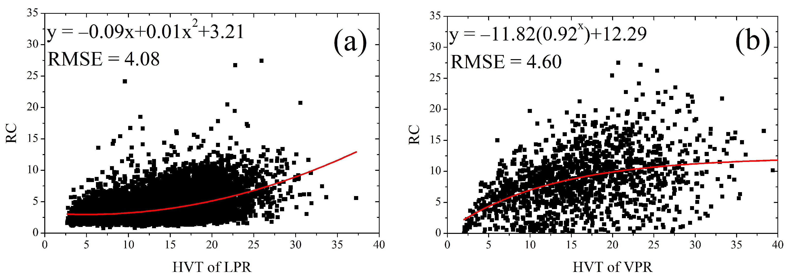
| Variables | Default | LPR | VPR |
|---|---|---|---|
| HVT | 16.0 | HVT from LPR | HVT from VPR |
| RC | 1.4 | −0.09 × HVT + 0.01 × HVT + 3.21 | + 12.29 |
Publisher’s Note: MDPI stays neutral with regard to jurisdictional claims in published maps and institutional affiliations. |
© 2022 by the authors. Licensee MDPI, Basel, Switzerland. This article is an open access article distributed under the terms and conditions of the Creative Commons Attribution (CC BY) license (https://creativecommons.org/licenses/by/4.0/).
Share and Cite
Wu, G.; You, Y.; Yang, Y.; Cao, J.; Bai, Y.; Zhu, S.; Wu, L.; Wang, W.; Chang, M.; Wang, X. UAV-LiDAR Measurement of Vegetation Canopy Structure Parameters and Their Impact on Land–Air Exchange Simulation Based on Noah-MP Model. Remote Sens. 2022, 14, 2998. https://doi.org/10.3390/rs14132998
Wu G, You Y, Yang Y, Cao J, Bai Y, Zhu S, Wu L, Wang W, Chang M, Wang X. UAV-LiDAR Measurement of Vegetation Canopy Structure Parameters and Their Impact on Land–Air Exchange Simulation Based on Noah-MP Model. Remote Sensing. 2022; 14(13):2998. https://doi.org/10.3390/rs14132998
Chicago/Turabian StyleWu, Guotong, Yingchang You, Yibin Yang, Jiachen Cao, Yujie Bai, Shengjie Zhu, Liping Wu, Weiwen Wang, Ming Chang, and Xuemei Wang. 2022. "UAV-LiDAR Measurement of Vegetation Canopy Structure Parameters and Their Impact on Land–Air Exchange Simulation Based on Noah-MP Model" Remote Sensing 14, no. 13: 2998. https://doi.org/10.3390/rs14132998