
Assessing the Yield of Wheat Using Satellite Remote Sensing-Based Machine Learning Algorithms and Simulation Modeling

 ,
,  ,
, 
 ,
,  ,
,  ,
, 
Abstract
:
1. Introduction
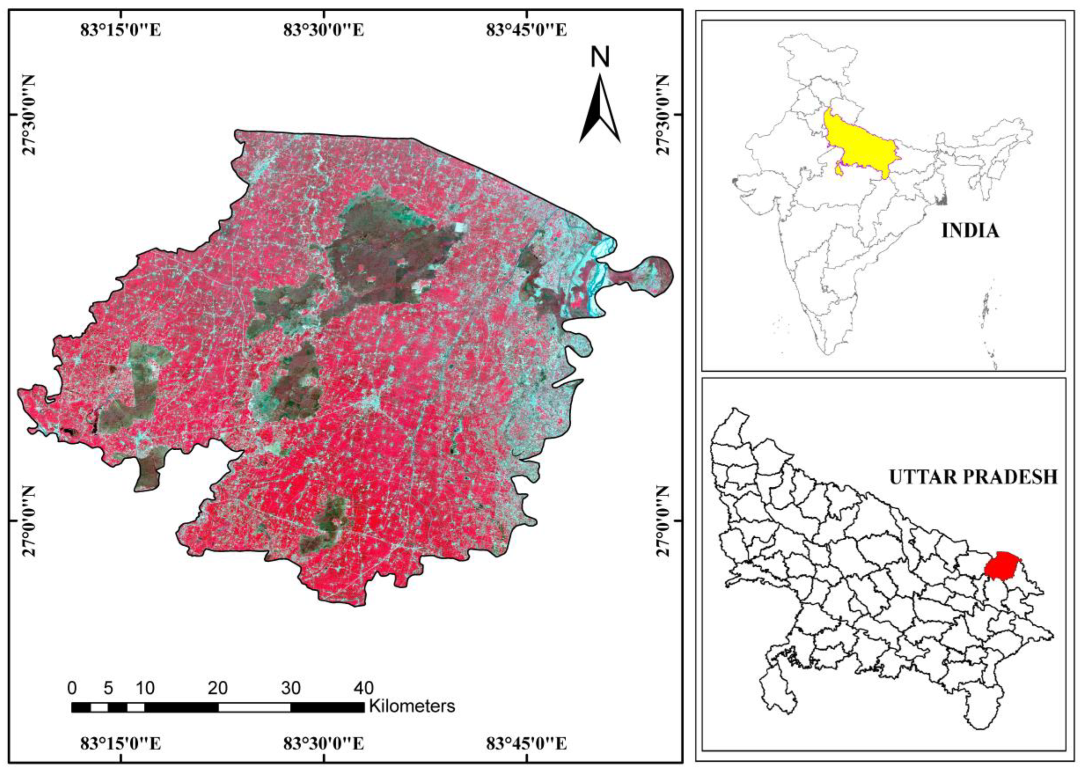
2. Study Area
3. Materials and Methods
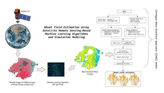
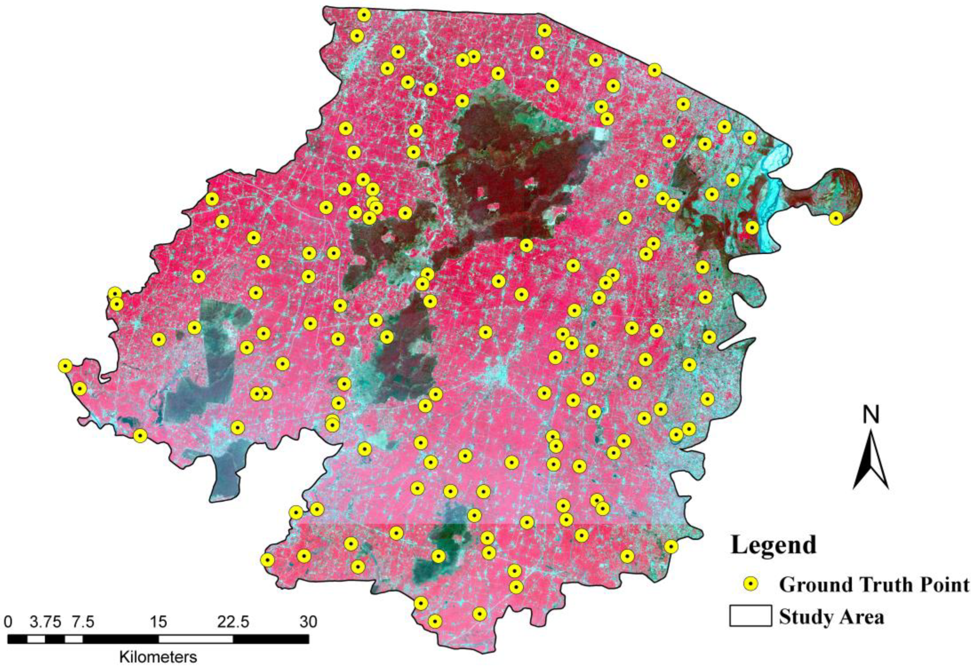
3.1. Datasets
3.2. Methods
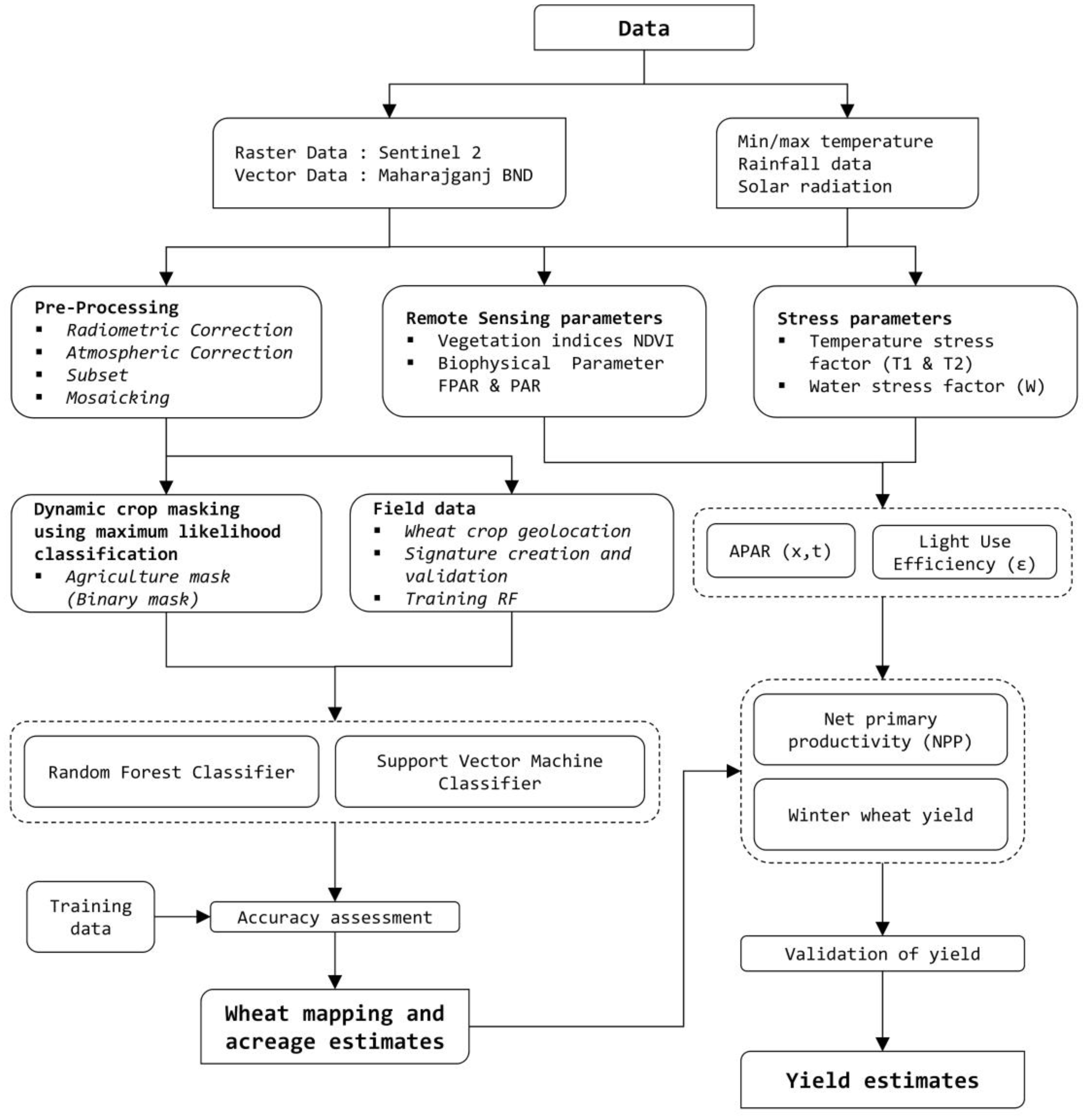
3.2.1. Acreage Estimation
3.2.2. Wheat Yield Estimation
4. Results and Discussion
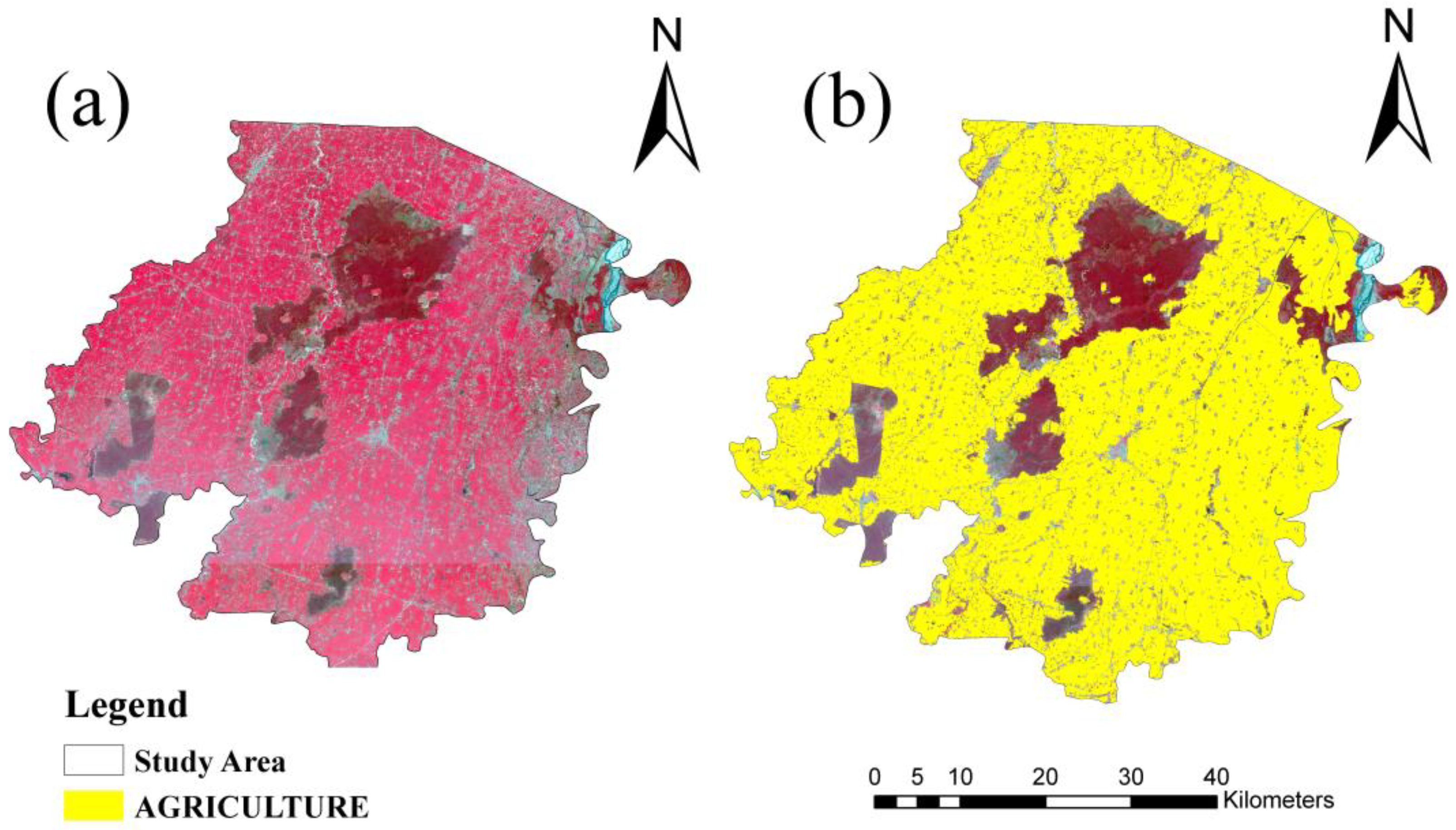
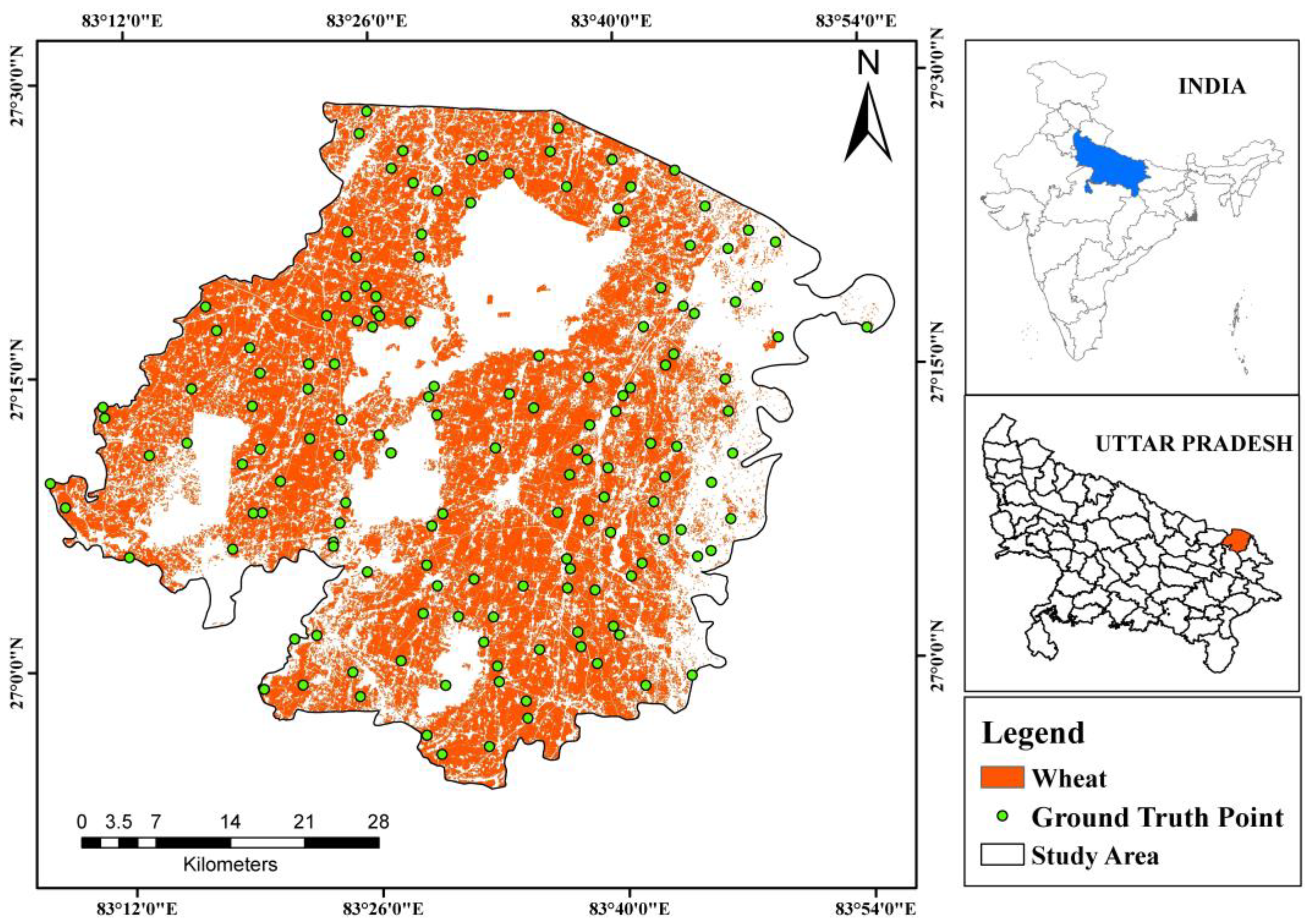
4.1. Wheat Acreage Estimation
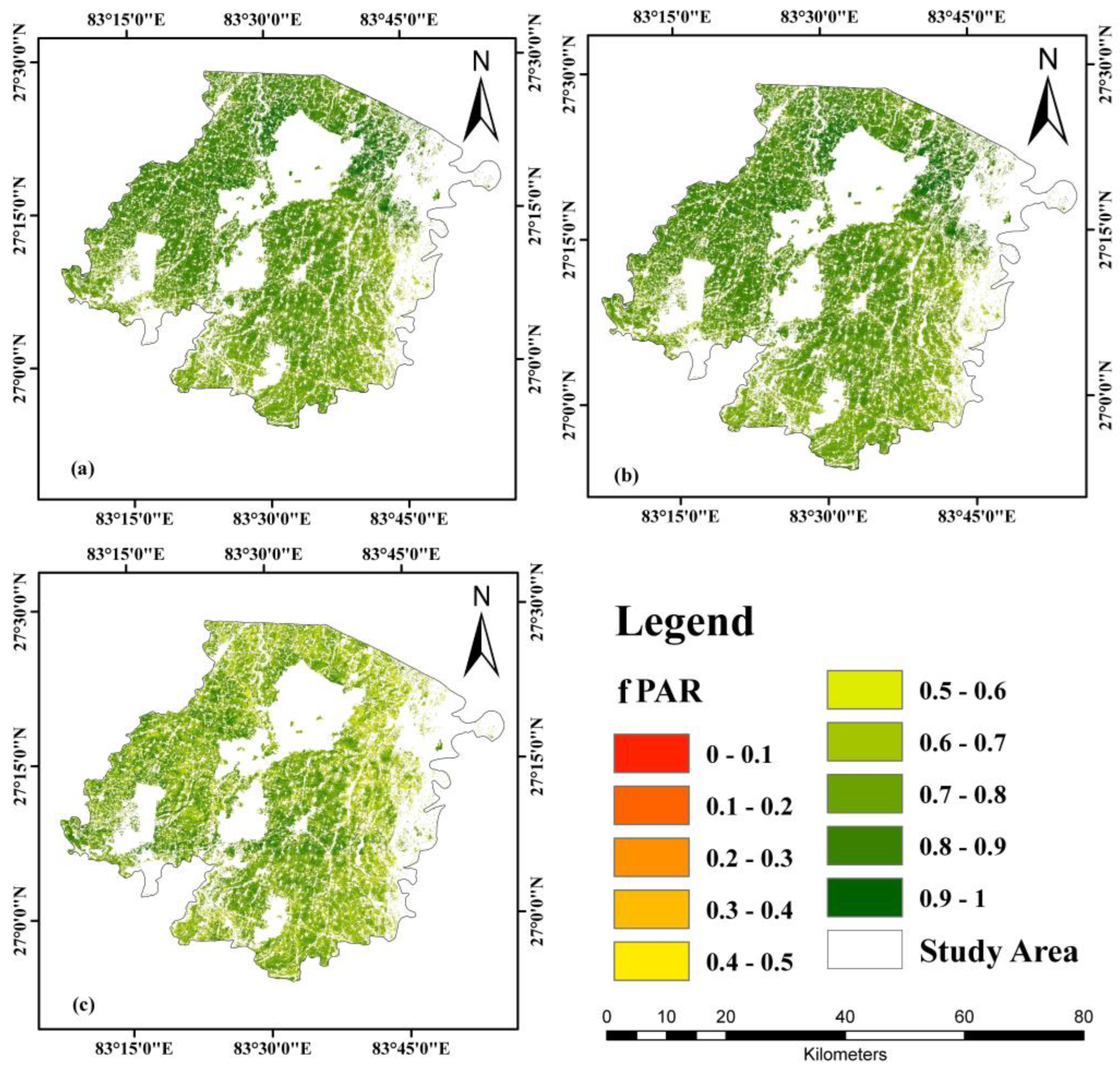
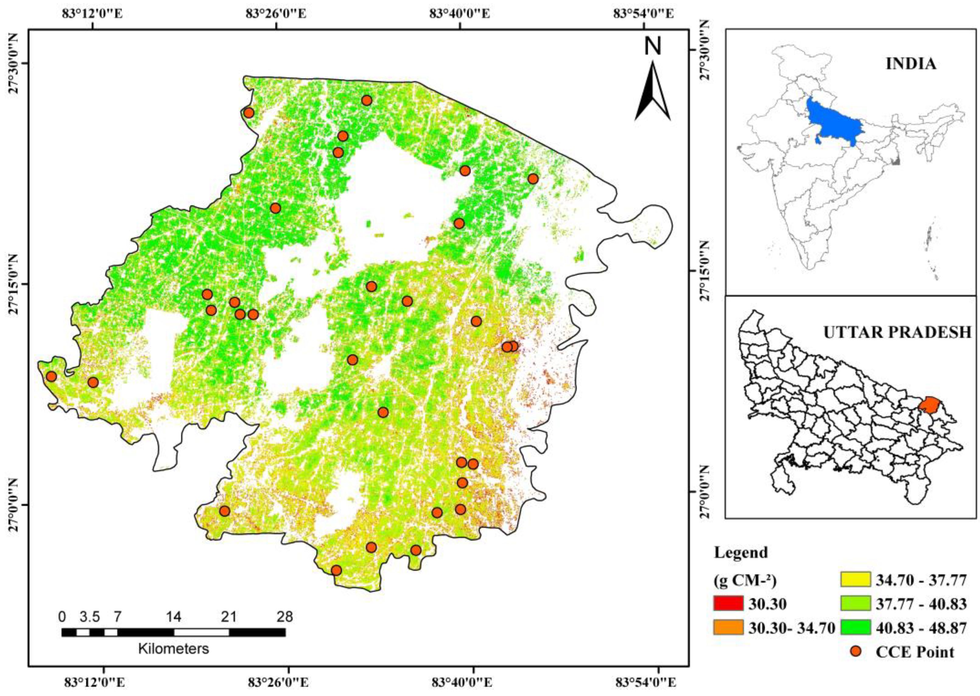
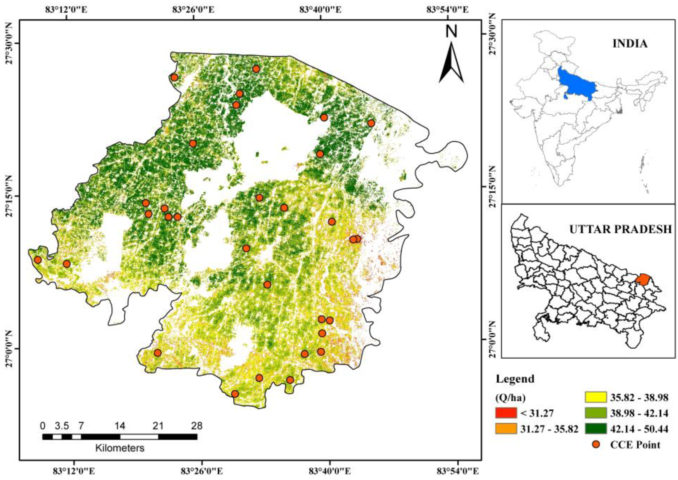
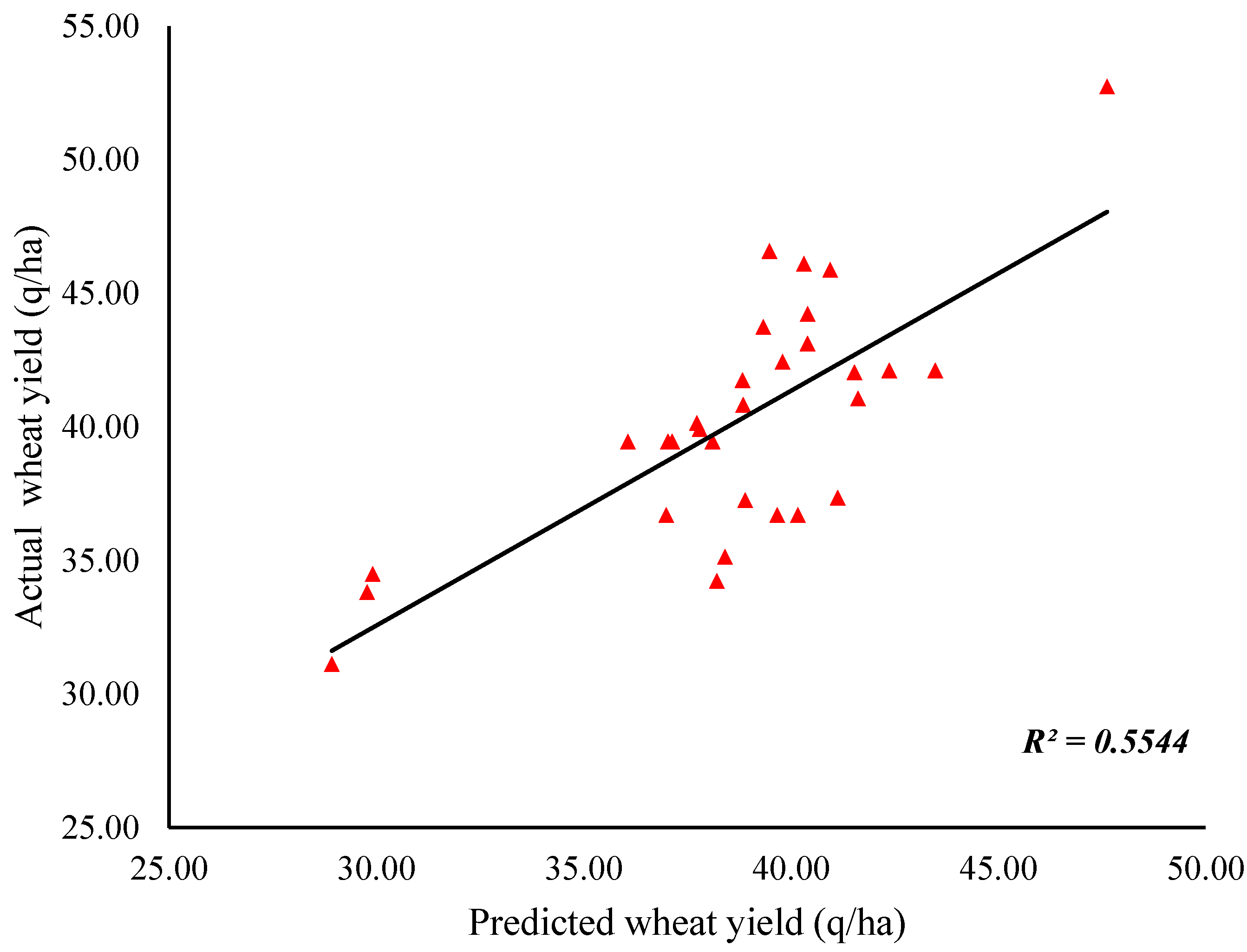
4.2. Wheat Yield Estimation Using the CASA Model
5. Conclusions
Author Contributions
Funding
Data Availability Statement
Acknowledgments
Conflicts of Interest
References
- Bolten, J.D.; Crow, W.T.; Zhan, X.; Jackson, T.J.; Reynolds, C.A. Evaluating the utility of remotely sensed soil moisture retrievals for operational agricultural drought monitoring. IEEE J. Sel. Top. Appl. Earth Obs. Remote Sens. 2009, 3, 57–66. [Google Scholar] [CrossRef] [Green Version]
- Chlingaryan, A.; Sukkarieh, S.; Whelan, B. Machine learning approaches for crop yield prediction and nitrogen status estimation in precision agriculture: A review. Comput. Electron. Agric. 2018, 151, 61–69. [Google Scholar] [CrossRef]
- Mateo-Sanchis, A.; Piles, M.; Muñoz-Marí, J.; Adsuara, J.E.; Pérez-Suay, A.; Camps-Valls, G. Synergistic integration of optical and microwave satellite data for crop yield estimation. Remote Sens. Environ. 2019, 234, 111460. [Google Scholar] [CrossRef] [PubMed]
- Zeng, N.; Zhao, F.; Collatz, G.J.; Kalnay, E.; Salawitch, R.J.; West, T.O.; Guanter, L. Agricultural Green Revolution as a driver of increasing atmospheric CO2 seasonal amplitude. Nature 2014, 515, 394–397. [Google Scholar]
- Lobell, D.B.; Burke, M.B. On the use of statistical models to predict crop yield responses to climate change. Agric. For. Meteorol. 2010, 150, 1443–1452. [Google Scholar] [CrossRef]
- Roberts, M.J.; Braun, N.O.; Sinclair, T.R.; Lobell, D.B.; Schlenker, W. Comparing and combining process-based crop models and statistical models with some implications for climate change. Environ. Res. Lett. 2017, 12, 095010. [Google Scholar] [CrossRef]
- Stehfest, E.; Heistermann, M.; Priess, J.A.; Ojima, D.S.; Alcamo, J. Simulation of global crop production with the ecosystem model DayCent. Ecol. Model. 2007, 209, 203–219. [Google Scholar] [CrossRef]
- Lamichhane, J.R.; Debaeke, P.; Steinberg, C.; You, M.P.; Barbetti, M.J.; Aubertot, J.N. Abiotic and biotic factors affecting crop seed germination and seedling emergence: A conceptual framework. Plant Soil 2018, 432, 1–28. [Google Scholar] [CrossRef]
- Lawless, C.; Semenov, M.A. Assessing lead-time for predicting wheat growth using a crop simulation model. Agric. For. Meteorol. 2005, 135, 302–313. [Google Scholar] [CrossRef]
- Orcutt, D.M.; Nilsen, E.T. Physiology of Plants under Stress: Soil and Biotic Factors; John Wiley & Sons: Hoboken, NJ, USA, 2000; Volume 2. [Google Scholar]
- Rembold, F.; Atzberger, C.; Savin, I.; Rojas, O. Using low resolution satellite imagery for yield prediction and yield anomaly detection. Remote Sens. 2013, 5, 1704–1733. [Google Scholar] [CrossRef] [Green Version]
- Gower, S.T.; Kucharik, C.J.; Norman, J.M. Direct and indirect estimation of leaf area index, fAPAR, and net primary production of terrestrial ecosystems. Remote Sens. Environ. 1999, 70, 29–51. [Google Scholar] [CrossRef]
- Kumar, A.; Giri, R.K.; Taloor, A.K.; Singh, A.K. Rainfall trend, variability and changes over the state of Punjab, India 1981–2020: A geospatial approach. Remote Sens. Appl. Soc. Environ. 2021, 23, 100595. [Google Scholar] [CrossRef]
- Meraj, G.; Farooq, M.; Singh, S.K.; Islam, M.; Kanga, S. Modeling the sediment retention and ecosystem provisioning services in the Kashmir valley, India, Western Himalayas. Model. Earth Syst. Environ. 2021, 1–26. [Google Scholar] [CrossRef]
- Penuelas, J.; Filella, I. Visible and near-infrared reflectance techniques for diagnosing plant physiological status. Trends Plant Sci. 1998, 3, 151–156. [Google Scholar] [CrossRef]
- Singh, S.K.; Meraj, G.; Mondal, N.; Bera, A.; Verma, M.K.; Tomar, J.S.; Kanga, S. Assessment of seasonal vegetation dynamics over parts of thar desert using geospatial techniques. J. Res. ANGRAU 2021, 49, 105–109. [Google Scholar]
- Technow, F.; Messina, C.D.; Totir, L.R.; Cooper, M. Integrating crop growth models with whole genome prediction through approximate Bayesian computation. PLoS ONE 2015, 10, e0130855. [Google Scholar]
- Raza, S.M.; Mahmood, S.A. Estimation of net rice production through improved CASA model by addition of soil suitability constant (ħα). Sustainability 2018, 10, 1788. [Google Scholar] [CrossRef] [Green Version]
- Li, Z.; Taylor, J.; Yang, H.; Casa, R.; Jin, X.; Li, Z.; Song, X.; Yang, G. A hierarchical interannual wheat yield and grain protein prediction model using spectral vegetative indices and meteorological data. Field Crops Res. 2020, 248, 107711. [Google Scholar] [CrossRef]
- Ahlawat, A.; Bhat, A.; Gupta, V.; Sharma, M.; Sharma, S.; Rai, S.K.; Singh, S.P. Market Share and Promotional Approaches of Pesticide Companies for Vegetable Crops in Jammu District. Int. J. Soc. Sci. 2021, 10, 115–121. [Google Scholar] [CrossRef]
- Renwick, A.; Dynes, R.; Johnstone, P.; King, W.; Holt, L.; Penelope, J. Challenges and opportunities for land use transformation: Insights from the Central Plains Water scheme in New Zealand. Sustainability 2019, 11, 4912. [Google Scholar] [CrossRef] [Green Version]
- Eli-Chukwu, N.C. Applications of artificial intelligence in agriculture: A review. Eng. Technol. Appl. Sci. Res. 2019, 9, 4377–4383. [Google Scholar] [CrossRef]
- Saini, R.; Ghosh, S.K. Crop classification on single date sentinel-2 imagery using random forest and suppor vector machine. Int. Arch. Photogramm. Remote Sens. Spat. Inf. Sci. 2018, 42, 683–688. [Google Scholar] [CrossRef] [Green Version]
- Ge, G.; Shi, Z.; Zhu, Y.; Yang, X.; Hao, Y. Land use/cover classification in an arid desert-oasis mosaic landscape of China using remote sensed imagery: Performance assessment of four machine learning algorithms. Glob. Ecol. Conserv. 2020, 22, e00971. [Google Scholar] [CrossRef]
- Mehrotra, S. The cornerstone of a planning strategy for the 21st Century. In Planning in the 20th Century and Beyond: India’s Planning Commission and the NITI Aayog; Cambridge University Press: Cambridge, UK, 2020; p. 208. [Google Scholar]
- Asseng, S.; Ewert, F.; Rosenzweig, C.; Jones, J.W.; Hatfield, J.L.; Ruane, A.C.; Boote, K.J.; Thorburn, P.J.; Rötter, R.P.; Cammarano, D.; et al. Uncertainty in simulating wheat yields under climate change. Nat. Clim. Chang. 2013, 3, 827–832. [Google Scholar] [CrossRef] [Green Version]
- Meraj, G.; Singh, S.K.; Kanga, S.; Islam, M. Modeling on comparison of ecosystem services concepts, tools, methods and their ecological-economic implications: A review. Model. Earth Syst. Environ. 2022, 8, 15–34. [Google Scholar]
- Jain, H. Trade Liberalization, Economic Growth and Environmental Externalities: An Analysis of Indian Manufacturing Industries; Springer: Singapore, 2016. [Google Scholar]
- Patel, N.R.; Dadhwal, V.K.; Saha, S.K.; Garg, A.; Sharma, N. Evaluation of MODIS data potential to infer water stress for wheat NPP estimation. Trop. Ecol. 2010, 51, 93. [Google Scholar]
- Mangiameli, M.; Mussumeci, G.; Gagliano, A. Evaluation of the Urban Microclimate in Catania using Multispectral Remote Sensing and GIS Technology. Climate 2022, 10, 18. [Google Scholar] [CrossRef]
- Kiefer, M.T.; Andresen, J.A.; Doubler, D.; Pollyea, A. Development of a gridded reference evapotranspiration dataset for the Great Lakes region. J. Hydrol. Reg. Stud. 2019, 24, 100606. [Google Scholar] [CrossRef]
- Taloor, A.K.; Kumar, V.; Singh, V.K.; Singh, A.K.; Kale, R.V.; Sharma, R.; Khajuria, V.; Raina, G.; Kouser, B.; Chowdhary, N.H. Land use land cover dynamics using remote sensing and GIS Techniques in Western Doon Valley, Uttarakhand, India. In Geoecology of Landscape Dynamics; Springer: Singapore, 2020; pp. 37–51. [Google Scholar]
- Khan, A.; Govil, H.; Taloor, A.K.; Kumar, G. Identification of artificial groundwater recharge sites in parts of Yamuna River basin India based on Remote Sensing and Geographical Information System. Groundw. Sustain. Dev. 2020, 11, 100415. [Google Scholar] [CrossRef]
- Bera, A.; Taloor, A.K.; Meraj, G.; Kanga, S.; Singh, S.K.; Đurin, B.; Anand, S. Climate vulnerability and economic determinants: Linkages and risk reduction in Sagar Island, India; A geospatial approach. Quat. Sci. Adv. 2021, 4, 100038. [Google Scholar] [CrossRef]
- Qadir, A.; Mondal, P. Synergistic use of radar and optical satellite data for improved monsoon cropland mapping in India. Remote Sens. 2020, 12, 522. [Google Scholar] [CrossRef] [Green Version]
- Guptha, G.C.; Swain, S.; Al-Ansari, N.; Taloor, A.K.; Dayal, D. Assessing the role of SuDS in resilience enhancement of urban drainage system: A case study of Gurugram City, India. Urban Clim. 2022, 41, 101075. [Google Scholar] [CrossRef]
- Romshoo, S.A.; Fayaz, M.; Meraj, G.; Bahuguna, I.M. Satellite-observed glacier recession in the Kashmir Himalaya, India, from 1980 to 2018. Environ. Monit. Assess. 2020, 192, 1–17. [Google Scholar] [CrossRef]
- Farooq, M.; Meraj, G.; Kanga, S.; Nathawat, R.; Singh, S.K.; Ranga, V. Slum Categorization for Efficient Development Plan—A Case Study of Udhampur City, Jammu and Kashmir Using Remote Sensing and GIS. In Geospatial Technology for Landscape and Environmental Management; Springer: Singapore, 2022; pp. 283–299. [Google Scholar]
- Verma, U.; Dabas, D.S.; Hooda, R.S.; Kalubarme, M.H.; Yadav, M.; Grewal, M.S.; Sharma, M.P.; Prawasi, R. Remote sensing based wheat acreage and spectral-trend-agrometeorological Yield Forecasting: Factor Analysis Approach. Stat. Appl. 2011, 9, 1–13. [Google Scholar]
- Konda, V.G.R.K.; Chejarla, V.R.; Mandla, V.R.; Voleti, V.; Chokkavarapu, N. Vegetation damage assessment due to Hudhud cyclone based on NDVI using Landsat-8 satellite imagery. Arab. J. Geosci. 2018, 11, 35. [Google Scholar] [CrossRef]
- Phalke, A.R.; Özdoğan, M.; Thenkabail, P.S.; Erickson, T.; Gorelick, N.; Yadav, K.; Congalton, R.G. Mapping croplands of Europe, middle east, Russia, and central Asia using Landsat, random forest, and google earth engine. ISPRS J. Photogramm. Remote Sens. 2020, 167, 104–122. [Google Scholar] [CrossRef]
- Dimitrov, P.; Dong, Q.; Eerens, H.; Gikov, A.; Filchev, L.; Roumenina, E.; Jelev, G. Sub-pixel crop type classification using PROBA-V 100 m NDVI time series and reference data from Sentinel-2 classifications. Remote Sens. 2019, 11, 1370. [Google Scholar] [CrossRef] [Green Version]
- Górriz, J.M.; Ramírez, J.; Suckling, J.; Illan, I.A.; Ortiz, A.; Martínez-Murcia, F.J.; Segovia, F.; Salas-Gonzalez, D.; Wang, S. Case-based statistical learning: A non-parametric implementation with a conditional-error rate SVM. IEEE Access 2017, 5, 11468–11478. [Google Scholar] [CrossRef]
- Hasan, M.A.M.; Nasser, M.; Pal, B.; Ahmad, S. Support vector machine and random forest modeling for intrusion detection system (IDS). J. Intell. Learn. Syst. Appl. 2014, 6, 42869. [Google Scholar] [CrossRef] [Green Version]
- Xu, Y.; Yu, L.; Zhao, F.R.; Cai, X.; Zhao, J.; Lu, H.; Gong, P. Tracking annual cropland changes from 1984 to 2016 using time-series Landsat images with a change-detection and post-classification approach: Experiments from three sites in Africa. Remote Sens. Environ. 2018, 218, 13–31. [Google Scholar] [CrossRef]
- Do, T.N.; Lenca, P.; Lallich, S.; Pham, N.K. Classifying very-high-dimensional data with random forests of oblique decision trees. In Advances in Knowledge Discovery and Management; Springer: Berlin/Heidelberg, Germany, 2010; pp. 39–55. [Google Scholar]
- Wang, X.; Liu, T.; Zheng, X.; Peng, H.; Xin, J.; Zhang, B. Short-term prediction of groundwater level using improved random forest regression with a combination of random features. Appl. Water Sci. 2018, 8, 125. [Google Scholar] [CrossRef] [Green Version]
- Hastie, T.; Tibshirani, R.; Friedman, J. Random forests. In The Elements of Statistical Learning; Springer: New York, NY, USA, 2009; pp. 587–604. [Google Scholar]
- Watts, J.D. Satellite Monitoring of Cropland-Related Carbon Sequestration Practices in North Central Montana. Ph.D. Thesis, College of Agriculture, Montana State University, Bozeman, MT, USA, 2008. [Google Scholar]
- Kanga, S.; Singh, S.K.; Meraj, G.; Kumar, A.; Parveen, R.; Kranjčić, N.; Đurin, B. Assessment of the Impact of Urbanization on Geoenvironmental Settings Using Geospatial Techniques: A Study of Panchkula District, Haryana. Geographies 2022, 2, 1–10. [Google Scholar] [CrossRef]
- Shyam, M.; Meraj, G.; Kanga, S.; Farooq, M.; Singh, S.K.; Sahu, N.; Kumar, P. Assessing the Groundwater Reserves of the Udaipur District, Aravalli Range, India, Using Geospatial Techniques. Water 2022, 14, 648. [Google Scholar] [CrossRef]
- Piñeiro, G.; Oesterheld, M.; Paruelo, J.M. Seasonal variation in aboveground production and radiation-use efficiency of temperate rangelands estimated through remote sensing. Ecosystems 2006, 9, 357–373. [Google Scholar] [CrossRef]
- Prince, S.D.; Goward, S.N. Global primary production: A remote sensing approach. J. Biogeogr. 1995, 22, 815–835. [Google Scholar] [CrossRef]
- Zhao, L.; Liu, Z.; Xu, S.; He, X.; Ni, Z.; Zhao, H.; Ren, S. Retrieving the diurnal FPAR of a maize canopy from the jointing stage to the tasseling stage with vegetation indices under different water stresses and light conditions. Sensors 2018, 18, 3965. [Google Scholar] [CrossRef] [Green Version]
- Guang-Sheng, Z.; Xin-Shi, Z. A natural vegetation NPP model. Chin. J. Plant Ecol. 1995, 19, 193. [Google Scholar]
- Ye, X.C.; Meng, Y.K.; Xu, L.G.; Xu, C.Y. Net primary productivity dynamics and associated hydrological driving factors in the floodplain wetland of China’s largest freshwater lake. Sci. Total Environ. 2019, 659, 302–313. [Google Scholar] [CrossRef]
- Nayak, R.K.; Patel, N.R.; Dadhwal, V.K. Estimation and analysis of terrestrial net primary productivity over India by remote-sensing-driven terrestrial biosphere model. Environ. Monit. Assess. 2010, 170, 195–213. [Google Scholar] [CrossRef]
- Coventry, D.R.; Gupta, R.K.; Yadav, A.; Poswal, R.S.; Chhokar, R.S.; Sharma, R.K.; Yadav, V.K.; Gill, S.C.; Kumar, A.; Mehta, A.; et al. Wheat quality and productivity as affected by varieties and sowing time in Haryana, India. Field Crops Res. 2011, 123, 214–225. [Google Scholar] [CrossRef]
- Singh, K.M.; Singh, A. Lentil in India: An Overview. 2014. Available online: https://papers.ssrn.com/sol3/papers.cfm?abstract_id=2510906 (accessed on 21 April 2022).
- Barma, N.C.D.; Hossain, A.; Hakim, M.; Mottaleb, K.A.; Alam, M.; Reza, M.; Ali, M.; Rohman, M. Progress and challenges of wheat production in the era of climate change: A Bangladesh perspective. In Wheat Production in Changing Environments; Springer: Singapore, 2019; pp. 615–679. [Google Scholar]
- Lambert, M.J.; Traoré, P.C.S.; Blaes, X.; Baret, P.; Defourny, P. Estimating smallholder crops production at village level from Sentinel-2 time series in Mali’s cotton belt. Remote Sens. Environ. 2018, 216, 647–657. [Google Scholar] [CrossRef]
- Field, C.B.; Randerson, J.T.; Malmström, C.M. Global net primary production: Combining ecology and remote sensing. Remote Sens. Environ. 1995, 51, 74–88. [Google Scholar] [CrossRef] [Green Version]
- Ajour, S. Evaluation of FAO’s Water Productivity Portal (WaPOR) Yield over the Beqaa Valley, Lebanon. Master’s Thesis, American University of Beirut, Beirut, Lebanon, 2021. Available online: https://scholarworks.aub.edu.lb/bitstream/handle/10938/22922/AjourSalma_2021.pdf?sequence=3 (accessed on 25 May 2022).
- Yao, F.; Tang, Y.; Wang, P.; Zhang, J. Estimation of maize yield by using a process-based model and remote sensing data in the Northeast China Plain. Phys. Chem. Earth Parts A B C 2015, 87, 142–152. [Google Scholar] [CrossRef]
- Bhatt, R.; Kaur, R.; Ghosh, A. Strategies to practice climate-smart agriculture to improve the livelihoods under the rice-wheat cropping system in South Asia. In Sustainable Management of Soil and Environment; Springer: Singapore, 2019; pp. 29–71. [Google Scholar]
- Sure, A.; Dikshit, O. Estimation of root zone soil moisture using passive microwave remote sensing: A case study for rice and wheat crops for three states in the Indo-Gangetic basin. J. Environ. Manag. 2019, 234, 75–89. [Google Scholar] [CrossRef] [PubMed]
- Gumma, M.K.; Kadiyala, M.D.M.; Panjala, P.; Ray, S.S.; Akuraju, V.R.; Dubey, S.; Smith, A.P.; Das, R.; Whitbread, A.M. Assimilation of remote sensing data into crop growth model for yield estimation: A case study from India. J. Indian Soc. Remote Sens. 2022, 50, 257–270. [Google Scholar] [CrossRef]
- Shi, S.; Ye, Y.; Xiao, R. Evaluation of Food Security Based on Remote Sensing Data—Taking Egypt as an Example. Remote Sens. 2022, 14, 2876. [Google Scholar] [CrossRef]
- Wang, Y.; Xu, X.; Huang, L.; Yang, G.; Fan, L.; Wei, P.; Chen, G. An improved CASA model for estimating winter wheat yield from remote sensing images. Remote Sens. 2019, 11, 1088. [Google Scholar] [CrossRef] [Green Version]
- Wu, C.; Chen, K.; You, X.; He, D.; Hu, L.; Liu, B.; Wang, R.; Shi, Y.; Li, C.; Liu, F. Improved CASA model based on satellite remote sensing data: Simulating net primary productivity of Qinghai Lake Basin alpine grassland. Geosci. Model Dev. Discuss. 2022, 10, 1–24. [Google Scholar]
- Wu, K.; Zhou, C.; Zhang, Y.; Xu, Y. Long-Term Spatiotemporal Variation of Net Primary Productivity and Its Correlation with the Urbanization: A Case Study in Hubei Province, China. Front. Environ. Sci. 2022, 9, 656. [Google Scholar] [CrossRef]


| Sr No | District | Taluka | Wheat Crop Area (ha) SVM | Percentage in the District | Wheat Crop Area (ha) RF | Percentage in the District |
|---|---|---|---|---|---|---|
| 1 | Maharajganj | Nautanwa | 36,850 | 25% | 35,229 | 24% |
| 2 | Mahrajganj | 21,673 | 15% | 20,702 | 14% | |
| 3 | Pharenda | 27,671 | 19% | 27,983 | 19% | |
| 4 | Nichaul | 62,672 | 42% | 62,585 | 43% | |
| Total Wheat Area (ha) | 148,866 | 100% | 148,866 | 100% | ||
| Classifier | User’s Accuracy | Producer’s Accuracy | Overall Accuracy | Kappa Estimates |
|---|---|---|---|---|
| SVM | 87.14% | 91.04% | 85.35% | 0.68 |
| RF | 94.29% | 95.65% | 93.20% | 0.84 |
| Crop | Average of Predicted Yield 2020–2021 (Q/Ha) | Average of Actual Yield Acquire from CCE (Q/Ha) | Relative Deviation (%) |
|---|---|---|---|
| Wheat | 38.46 | 40.23 | −4.61% |
Publisher’s Note: MDPI stays neutral with regard to jurisdictional claims in published maps and institutional affiliations. |
© 2022 by the authors. Licensee MDPI, Basel, Switzerland. This article is an open access article distributed under the terms and conditions of the Creative Commons Attribution (CC BY) license (https://creativecommons.org/licenses/by/4.0/).
Share and Cite
Meraj, G.; Kanga, S.; Ambadkar, A.; Kumar, P.; Singh, S.K.; Farooq, M.; Johnson, B.A.; Rai, A.; Sahu, N. Assessing the Yield of Wheat Using Satellite Remote Sensing-Based Machine Learning Algorithms and Simulation Modeling. Remote Sens. 2022, 14, 3005. https://doi.org/10.3390/rs14133005
Meraj G, Kanga S, Ambadkar A, Kumar P, Singh SK, Farooq M, Johnson BA, Rai A, Sahu N. Assessing the Yield of Wheat Using Satellite Remote Sensing-Based Machine Learning Algorithms and Simulation Modeling. Remote Sensing. 2022; 14(13):3005. https://doi.org/10.3390/rs14133005
Chicago/Turabian StyleMeraj, Gowhar, Shruti Kanga, Abhijeet Ambadkar, Pankaj Kumar, Suraj Kumar Singh, Majid Farooq, Brian Alan Johnson, Akshay Rai, and Netrananda Sahu. 2022. "Assessing the Yield of Wheat Using Satellite Remote Sensing-Based Machine Learning Algorithms and Simulation Modeling" Remote Sensing 14, no. 13: 3005. https://doi.org/10.3390/rs14133005