Article

Estimation of Canopy Structure of Field Crops Using Sentinel-2 Bands with Vegetation Indices and Machine Learning Algorithms

1
School of Remote Sensing and Geomatics Engineering, Nanjing University of Information Science and Technology, Nanjing 210044, China
2
VTT Technical Research Centre of Finland Ltd., FI-02044 Espoo, Finland
*
Author to whom correspondence should be addressed.
Remote Sens. 2022, 14(12), 2849; https://doi.org/10.3390/rs14122849
Submission received: 10 May 2022 / Revised: 11 June 2022 / Accepted: 13 June 2022 / Published: 14 June 2022

Abstract

:
Leaf angle distribution (LAD), or the leaf mean tilt angle (MTA) capturing its central value, is used to quantify the direction of the leaf surface in a canopy and is one of the most important canopy structuraltraits. Combined with the other important structure parameter, leaf area index (LAI), LAD determines the light interception of a crop canopy. However, unlike LAI, only few studies have addressed the direct retrieval of LAD or MTA from remote sensing data. Recently, it has been shown that the red edge is a key spectral region where the effect of leaf angle on crop spectral reflectance can be separated from that of other structural variables. The Multispectral imager (MSI) onboard the Sentinel-2 (S2) satellite has two specially designed red-edge channels in this spectral region and thus can potentially be used for large-scale mapping of MTA at high spatial and temporal resolutions. Unfortunately, no field data on leaf angles at the scale of S2 pixel are available. Therefore, we simulated 5000 observations of different crops using the PROSAIL canopy reflectance model. Further, we used the MTA and LAI data of six crop species growing in 162 experimental plots in Finland and simulated their reflectance signal in S2 bands by resampling AISA airborne imaging spectroscopy data. Four common machine learning regression algorithms (random forest, support vector machine, multilayer perceptron network and partial least squares regression) were examined for retrieving canopy structure parameters, including leaf angle, from the simulated reflectances. Further, we analyzed the utility of 12 vegetation indices (VIs) well known to be sensitive to canopy structure for canopy structure estimation. Six of the studied indices used information from the visible part of the spectrum and the near infrared (NIR) while another six were selected to also utilize the red edge bands specific to S2. We found that S2 band 6 in the red edge had a strong correlation with MTA (R2 = 0.79 in model simulation and R2 = 0.87 in field measurements) but a low correlation with LAI (R2 = 0.07 in model simulation and R2= 0.06 in field measurements). Of the six red edge-based VIs, four (NDVIRE, CIRE, WDRVIRE and MSRRE) depended less on MTA than the visible NIR-based VIs and thus could be useful for estimating LAI for any LAD. The other two red edge-based VIs, IRECI and S2REP, had stronger correlations with MTA (R2 = 0.67 and 0.52, respectively) than LAI (R2 = 0.24 and 0.19, respectively). Additionally, MTA was accurately estimated (RMSE = 1.1–2.4° in model simulations and RMSE = 2.2–3.9° in field measurements) using the four 10 m spatial resolution bands with the RF, SVM and MLP algorithms, without information in the red edge. These promising results indicate the capability of S2 in accurately mapping the MTA of field crops on a large scale.

Graphical Abstract

1. Introduction

The structure of a plant canopy is determined by the amount and spatial organization of plant elements above the ground. It directly affects the proportion of solar energy intercepted by the canopy, its photosynthetic activity and ultimately productivity [1,2,3]. Assuming the canopy to be spatially continuous and horizontally homogeneous—common assumptions for field crops—its structure can be accurately described by the leaf area index (LAI) and leaf inclination angle distribution (LAD) [4,5]. Vegetation LAI and LAD are affected by biome, genotype and growth condition and jointly determine the fraction of canopy cover (Fcover) of a continuous and horizontally homogeneous canopy.
LAI, the sum of single-sided vegetation leaf area per area unit of horizontal ground [6], is one of the most important canopy structural traits. It is an essential indicator of crop phonological status and is used widely in precision agriculture [7,8]. LAD quantifies the angle between the leaf surface normal and nadir directions, and is closely associated with canopy light interception. Steeper leaves (greater leaf inclination angle) in the topmost canopy decrease light interception and cause more light to be transmitted into the lower canopy layers and vice versa. LAD plays in important role in determining energy and mass balance intra- and inter-canopy. Potentially, it could also be used to help mapping species for which LAD intervals are most likely known, based on a geographic location or sensing time, or to map local variations in crop health or productivity.
Canopy structural variables, as important canopy characteristics and factors influencing canopy reflectance, have been in the focus of Earth observations [9,10]. Spectral vegetation indices (VIs), combination functions of reflectance in two or more wavebands, have been one of the most productive methods for monitoring the structure of field crops. Traditionally, the bands used in VIs are situated in visible and near-infrared spectral regions, making use of the absorption bands of the photosynthetic pigments. The purpose of combining reflectance values into VIs is to strengthen the sensitivity of the spectral signature to specific vegetation biophysical parameters and overcome the effects of other factors, e.g., atmospheric conditions, observation geometry and soil reflectance [11,12].
The simplest way of using VIs to predict canopy biophysical properties is regressing them against the VIs using least squares [13,14,15]. However, it has been reported that machine learning (ML) methods, such as random forest (RF), artificial neural networks (ANNs), support vector machine (SVM) or partial least squares regression (PLSR) can estimate plant biophysical and biochemical parameters more accurately from remote sensing data [16,17,18,19,20] compared with least squares regression. ML can also use all available spectral bands or spectral features in establishing robust and nonlinear relationships.
Both LAI and LAD have a confounding influence on canopy reflectance. However, most work has focused on the retrieval of the leaf area index while ignoring LAD due to the absence of actual measurements of canopy leaf angles. In practical applications, LAD is usually assumed to be spherical with the leaf mean tilt angle (MTA) fixed to 57°. A rare example of studies focusing on leaf angles, the species-specific MTA of six crop species was retrieved from airborne imaging spectroscopy data using single spectral reflectance at 748 nm and two reflectance (663 and 445 nm) combinations, which produced R2 = 0.60 between the true and estimated MTA values [21].
Imaging spectroscopy data can provide detailed spectral traits [22], giving it a theoretical advantage over multispectral remote sensing for the detection of crop canopy features. However, concerning the technical implementation and sensor costs to track the temporal dynamics of canopy structure over large areas, especially global mapping, continuous satellite-based multispectral monitoring may be a better alternative for practical applications. An increasing number of satellites with moderate and fine spatial resolutions have become available in recent years, such as the Sentinel-2(S2) Multispectral Imager (MSI).The MSI sensors with two strategically designed red edge channels opened up opportunities for improving vegetation monitoring [23,24,25] and are very promising for the demand of precision agriculture. The spatial resolution of the vegetation bands of S2 is 10 m while the narrow red edge bands are provided at 20 m resolution. The current two S2 satellites were launched in 2015 and 2017 with an average global revisit interval of 5 days, allowing for operational detection of changes in crop structure.
The specific wavelength of 748 nm, which produced a strong relationship between MTA and reflectance [26], is not measured by multispectral satellite instruments. Fortunately, the S2 has a red edge band at 740 nm, encouraging us to test its capability in canopy MTA estimation. However, due to the lack of measurements of a wide range of crop structure variables, especially the leaf angle, at the scale of real S2 data, we could not test MTA estimation with real S2 imagery. Instead, we used band simulation, a common approach of resampling narrow-band reflectance [27,28], using the spectral response functions of a broadband sensor to obtain broadband reflectance. We used two sources of narrowband reflectance data: simulated using a well-tested physical vegetation reflectance model, and obtained over small test fields using an airborne hyperspectral scanner. The simulated dataset with a wide range of situations were used to evaluate the potential of S2 bands for estimating canopy structure in a more general and robust manner, and the empirical dataset was used to test the model simulated results.
We used the reflectance values in individual simulated bands as well as widely used vegetation indices computable from S2 data to test the potential of S2 in canopy MTA retrieval using ML algorithms. To test the spatial resolution achievable for leaf angle mapping with S2, we separately tested the bands at 10 m resolution and the visible and NIR bands with a resolution of 20 m or better.

2. Materials and Methods

2.1. Study Area and Field Measurements

We used the crop data from a test field (Figure 1) belonging to the University of Helsinki, Finland (60°13′26″ N, 25°1′16″ E). The area of the test field is approximately 4 × 4 km. The mean elevation of this area is approximately 10 m above sea level. The mean temperatures are 18 °C and 6 °C in July and throughout the year, respectively. Six crop species with a total of 162 plots were included in the used dataset, including narrow-leafed lupin (Lupinus angustifolius L. ‘HaagsBlaue’), faba bean (Vicia faba L. ‘Kontu’), wheat (Triticum aestivum L. emend Thell. ‘Amaretto’), turnip rape (Brassica rapa L. ssp. oleifera (DC.) Metzg. ‘Apollo’), barley (Hordeum vulgare L. ‘Streif’, ‘Chill’ and ‘Fairytale’) and oat (Avenasativa L. ‘Ivory’ and ‘Mirella’). These crops are representative species grown in cool-temperate regions. The sizes of the plots in the different agricultural experiments varied between 10 × 2 and 50 × 12 m2. Six species were planted with different densities varying between 55 and 700 m−2 and the fertilizer levels varied between 0 and 150 kg N m−2, which resulted in the variation in the leaf area index.The plots are described in detail in a previous study [26].
The canopy LAD of six crop species was acquired by a digital camera imaging approach [26] on 6 July 2012. The measurements were conducted at the same crop development stage one year after the canopy spectroscopic data acquisition. We also measured MTA in 2013 in the same growing stages and found no significant differences between the two years (data not shown). Images of the canopy were taken with a digital camera (Nikon D1X, Tokyo, Japan), which was attached and leveled on a tripod when photographs were taken. All the photographs were acquired at a distance of approximately one meter from the border of the plots. To ensure that the entire canopy was photographed, the camera height was adjusted according to the actual height of the plant with a variation between 30 and 50 cm. For each species, five to six photographs were acquired from one or several plots. By means of ImageJ software (version 1.47), 75 to 100 leaves or measurable leaf segment angles were measured from the photos for each species. The measurable leaf segments refer to the segment orientation perpendicular to the imaging direction and only for cereal crop species with long and narrow leaves. LAD or MTA is a highly species-specific trait, that differs more between species than within species [4,29,30]. This species-specific feature has been proved by remote sensing results [21]. In this study, we followed the advice of Piseket et al. [31] to use species-specific LAD, determined from actual leaf angle measurements.
The airborne hyperspectral data used in the study have been obtained using an AISA Eagle II imaging spectrometer (Specim, Oulu, Finland) equipped on a twin-engine aircraft on 25 July 2011, from approx. 600 m above ground, and reported in detail by Zou et al. [26] together with the field data. Here, we only summarize the dataset. The hyperspectral imagery contains 64 continuous bands in the visible to near infrared spectral regions, between 400 and 1000 nm, with a spectral resolution between 9 and 10 nm. The data had been georeferenced and processed to top-of-canopy hemispherical-directional reflectance factors using atmospheric aerosol data from a nearby AERONET sun photometer. Leaf area index data used in the study had been obtained using a SunScan SS1 device (Delta-T Devices, Cambridge, UK) within five days of the airborne campaign. The SunScan canopy analysis system measures radiation levels above and below a vegetation canopy, allowing us to estimate the intercepting leaf area. We used the species-specific leaf angle information determined from the photographs in converting the SunScan measurements of radiation interceptance to LAI using the equations provided in the SunScan user manual [32]. The LAI varied between 1.1 and 5 for the six crop species.The equations provided in the manual, based on the Beer-Lamber law, were also used to convert the canopy interceptance measured for the actual solar angle to zenith illumination, providing the canopy fractional cover, Fcover. The plots of the species used in the study were identified in the hyperspectral imagery using the agricultural field maps.
Soil reflectance was measured from four harvested plots using a handheld Analytical Spectral Device (ASD, Longmont, CO, USA) between 11:30 and 12:30 local time, on 7 October 2011. A white reference panel (Spectralon) was used to record reference spectra before and after soil spectral measurements. The soil reflectance was calculated as the ratio of the soil-reflected radiance to the reference radiance. The mean reflectance of the four plots was used as the soil reflectance of all the studied plots. Finally, the measured soil reflectance was calibrated using a bidirectional reflectance function model developed by Walthall et al. [33] and modified by Nilson and Kuusk [34] to coincide with the solar illumination conditions of airborne hyperspectral data acquisition. Due to the small study area, the measured soil spectral reflectance was assumed to be the same for all plots.

2.2. PROSAIL Model Application

The PROSAIL model is designed for horizontally homogeneous vegetation canopies and is suited for modeling the reflectance of field crops. It is a combination of PROSPECT-5 [35] and SAILH [36,37] model. PROSPECT-5 is a leaf optical properties model consisting of six input parameters: leaf structure parameter (N), leaf chlorophyll content (Cab), leaf carotenoid content (Car), leaf water content (Cw), leaf brown pigment content (Cbp) and leaf dry matter content (Cm). SAILH simulates the bidirectional reflectance of a homogenous canopy as a function of LAI, MTA, hot spot parameter, soil reflectance (ρsoil), the fraction of incident diffuse sky radiation(skyl) and three measurement geometry parameters: solar zenith angle (SZA), observation zenith angle(OZA) and relative azimuth angle (RAA). The range of model inputs was generalized from the measurements to represent the typical range for the peak growing season. Values of variables, which were not measured, were obtained from literature. The detailed description of the PROSAIL model inputs are given in Table 1. LAI varied between 1 and 5, MTA between 15 and 70 degrees, Cab between 25 and 100 μg cm−2 and Cw between 0.001 and 0.020. Car was linked to 20 percent of the Cab value based on the LOPEX93 dataset [38]. The other model inputs were fixed: Cbp = 0 (assuming no senescent leaves during field measurement), Cm = 0.005 g cm−2 (average value of the six crop species [39,40,41,42], N = 1.55 (average of various crop species [43], hot spot parameter was set to 0.01, skyl was calculated using 6S atmosphere radiative transfer model and ρsoil was acquired from actual ASD measurement. The three sun-senor geometry parameters were set to be consistent with the scenario of airborne measurements (SZA = 49.4°, OZA = 9° and RAA = 90°). All the flexible parameters were varied freely within a uniform distribution bounded by the range of each value and resulting in 5000 combinations. For each combination, canopy reflectance was simulated with 1 nm spectral resolution and resampled to S2 band reflectance (Section 2.3).

2.3. Simulation of Sentinel-2 Bands

To investigate the potential application of the widely used broadband satellite sensor Sentinel-2, airborne imaging spectroscopy data were resampled to multispectral according to the S2 sensor spectral response functions (Figure S1) with central wavelengths of 490, 560, 665, 705, 740, 783, 842 and 865 nm (Table 2). As we only had hyperspectral data in the visible and NIR spectral regions, we ignored the shortwave infrared (SWIR) bands of S2. The mean reflectance of the six crop species with S2 band central wavelengths is presented in Figure 2.

2.4. Vegetation Indices

In this study, 12 commonly used canopy structure-sensitive VIs were calculated using S2 bands (Table 3). Six VIs were calculated based on visible and NIR reflectance, including the normalized different vegetation index (NDVI) [44], the enhanced vegetation index (EVI) [45] and its two-band version (EVI2) [46], the second modified triangular vegetation index (MTVI2) incorporating a soil adjustment factor [43], the optimized soil adjusted vegetation index (OSAVI) [47] and the wide dynamic range vegetation index (WDRVI) [48,49]. These indices can be computed at 10 m spatial resolution. The other six indices, using both NIR and the red edge (available at 20 m resolution) reflectance include the red edge normalized difference vegetation index (NDVIRE) [50], chlorophyll index red-edge (CIRE) [51], modified simple ratio red-edge(MSRRE) [52,53,54], red-edge wide dynamic range vegetation index (WDRVIRE) [49], inverted red-edge chlorophyll index (IRECI) [55] and Sentinel-2 red-edge position (S2REP) [55]. The actual bands used for VI calculation are specified in Table 3.

2.5. Machine Learning Algorithms and Statistical Analysis

2.5.1. Implementation and Optimization

Four popular ML regression algorithms, Random Forest (RF), Support Vector Machine (SVM), multilayer perceptron(MLP) and Partial Least Squares Regression (PLSR), were compared and evaluated to predict three crop canopy structure parameters (LAI, MTA and Fcover) from either individual band reflectance or vegetation indices. When using reflectance data as ML input, two sets of input bands were used: (i) bands with a resolution of 10 m in S2 imagery, and (ii) bands with a resolution of 10 m or 20 m. To optimize the number of input VIs, vegetation indices were used in the model based on their ranks of R2 with the variable of interest (LAI, MTA or Fcover). In the first step, all twelve VIs were used as input features, and afterwards, the VIs which had less correlation with the variable of interest were progressively removed one by one until two VIs with the largest R2 remained. For empirical measurements, a leave-one-out approach was used for cross-validation to select the optimal tuning parameters for model optimization. In this method, only one sample is selected for verification and all other samples are taken as training samples [56]. A model was fitted repeatedly to a dataset containing n-1 observations (the number of observations, n = 162). For model simulation, 5-fold was used for cross-validation. In this method, all the data were partitioned into 5 sub samples with equal sizes and each sub sample was used for validation, and the other samples were used for training once, which means that the process was repeated 5 times.
A grid search method was employed to identify optimal configurations of tuning parameters for RF and SVM, which have two tuning parameters. The optimal evaluation is based on the cross-validated correlation between estimated and measured variables. The regression algorithm implementation was performed using the package scikit-learn in Python 3.5.

2.5.2. Random Forest (RF)

RF regression is a nonparametric and ensemble ML algorithm that comprises a large number (ntree) of decision trees without correlation between them [57]. In RF regression, a certain number of samples are randomly selected from the training set as the root node samples of each tree, and a regression tree is constructed to reduce the prediction error [58]. The optimal combination of tuning parameters (ntree and mtry) were determined using a grid search cross validation to identify the best settings for canopy structure parameter prediction. In this study, the tested combination values of ntree were set as 20, 50, 100, 200, 500, 1000 and 2000 and mtry was set between 2 and 8 with an interval of 1.

2.5.3. Support Vector Machine (SVM)

SVM has initially been developed for classification. The method was later extended for regression of nonlinear and high-dimensional samples [59] of continuous variables. The fundamental aspect of this algorithm is a statistical learning theory of structural risk minimization. The benefit of SVM regression is that it allows the construction of nonlinear models without changing explanatory variables, so it can better explain the generated models. By employing a kernel function, the initial multidimensional space with linear, nonseparable problems was projected to a higher dimensional feature space with a linear, separable feature space [60]. Based on this high-dimensional feature space where the original input data are mapped from a nonlinear function, support vector regression becomes a linear regression function. In this research, a commonly used radial basis function kernel was utilized for regression. Two tuning parameters in the kernel function were optimized to calibrate the model: one is the cost of constraint violation (C), and the other is the coefficient gamma (γ). The trade-off between the relaxation variable penalty and the width of the margin was determined by the parameter C, while the influence of a single training sample was determined by the parameter γ. The parameter C has a positive relationship with penalties for estimation error and overfitting of the model. The parameter γ determines the kernel function and overall estimation accuracy. In this study, the optimal configuration was determined using a grid search method. The tested combination values of C were set as 0.1, 0.3, 0.5, 0.8 and 1.0 and the coefficient gamma γ values were set as 0.05, 0.10, 0.15, 0.2, 0.25, 0.3, 0.5, 0.75 and 1.

2.5.4. Multilayer Perceptron (MLP)

The MLP is an artificial neural network, consisting of a large number of connected artificial neurons which propagate the signal in the system. MLP consists of three layers of nonlinear active nodes, including input, hidden and output layers. In the MLP model, the settings of the hidden layer were tuned which consisted of the number of hidden layers and perceptrons contained in each hidden layer. The tested node numbers were set to 2, 5, 10, 20, 50 and 100 for the single-layer mode, and the tested node combinations were (2, 2), (5, 5), (10, 10), (20, 20), (50, 50) and (100, 100) for the two-layer mode.

2.5.5. Partial Least Squares Regression (PLSR)

PLSR is a statistical method with multivariate analysis that combines the advantages of three analyses including multiple linear regression analysis, canonical correlation analysis and principal component analysis. It can deal with multidimensional and collinear datasets. When a linear relationship was established from multiple independent variables, it could efficiently evaluate their effects on a dependent variable [61]. The dimensionality of high-dimensional data could be reduced using principal component analysis. In this study, the number of tested principal components varied between 2 and 6.

2.5.6. Statistical Analysis

The coefficient of determination (R2), the root mean square error (RMSE), and the relative root mean square error (RRMSE) were used to evaluate the accuracy of each approach. The R2 value can explain the variation and predictive ability of the model. The RMSE and RRMSE indicate the difference and the relative differences between the measured and estimated values. They were calculated as follows:
R 2 = 1 - i = 1 n y i x i 2 i = 1 n y i y ¯ 2
RMSE = i = 1 n y i x i 2 n
RRMSE = RMSE y ¯
where x i indicates the model output value, y i is the measured value, y ¯ indicates the mean and n indicates the number of samples in the dataset.

3. Results

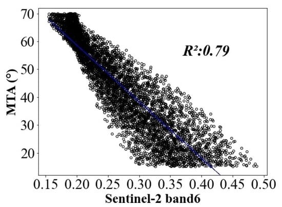
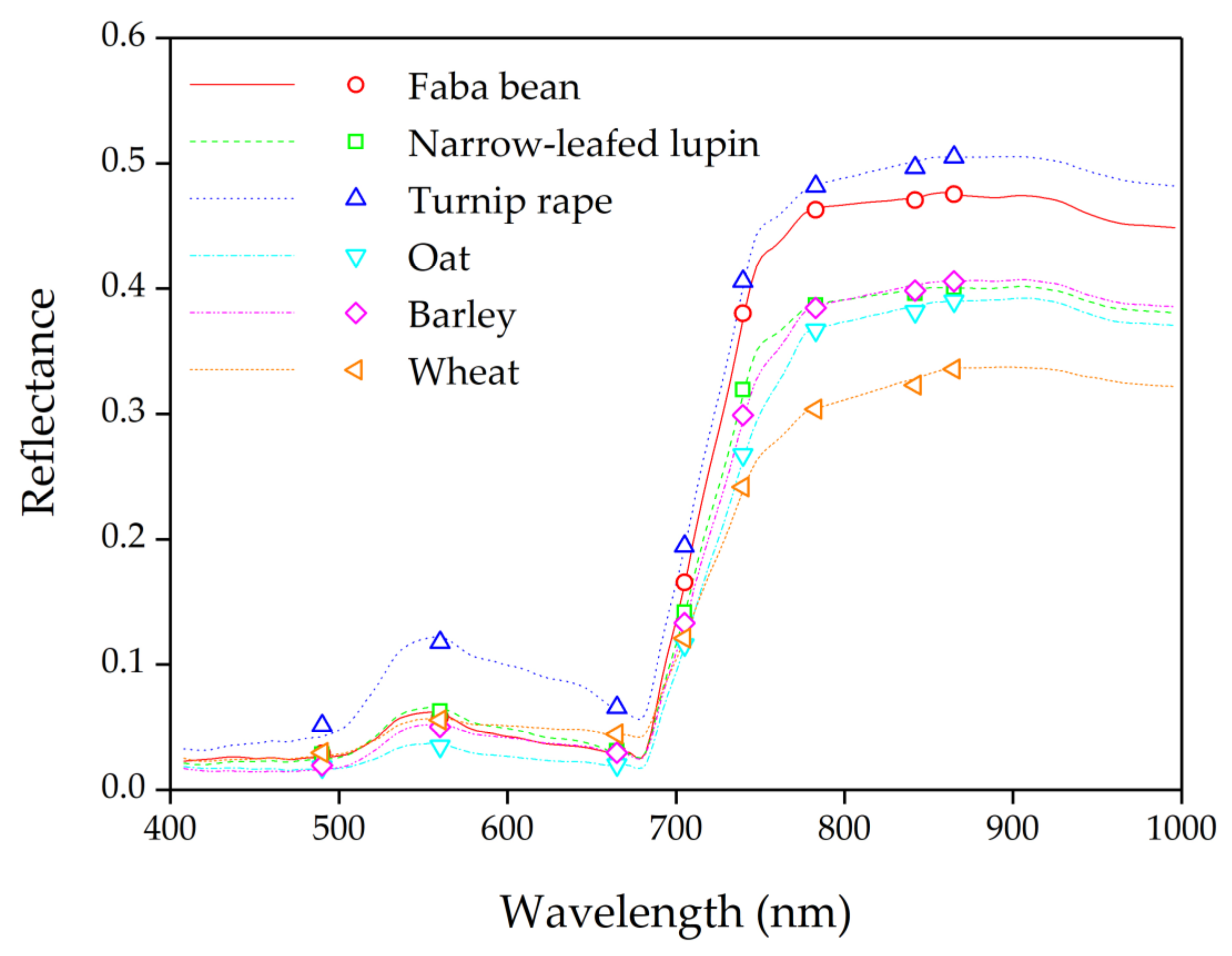
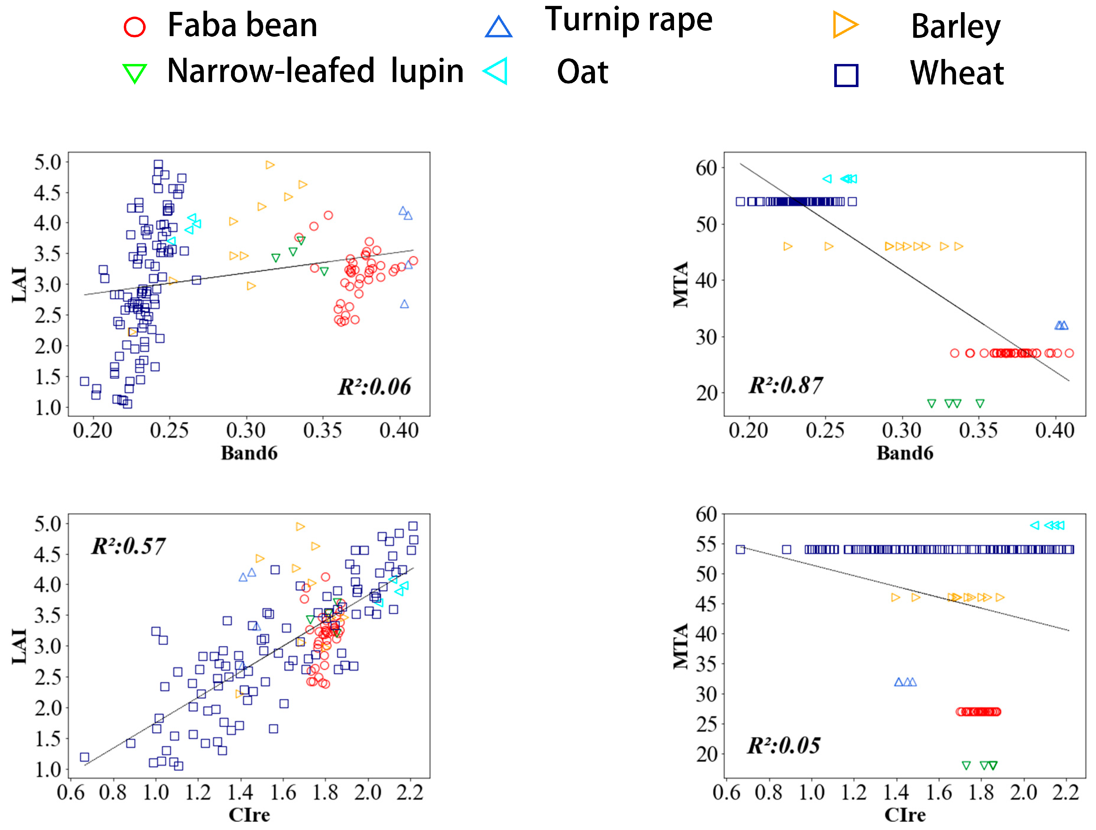
3.1. Correlations between Canopy Structural Characteristics and Remotely Sensed Data

The coefficients of determination between the S2 bands and canopy structure parameters are given in Table 4. S2 bands 2 and 4 (blue and red, respectively) had medium-strength correlations with LAI for both model simulations and empirical dataset. In AISA data, the correlations of these bands with MTA were very weak, but in model-simulated data, moderate correlations were found. S2 band 6 (RE2, 740 nm) produced the strongest correlation with MTA (R2 = 0.79 in PROSAIL simulations, 0.87 in AISA data in Figure 3) and little correlation with LAI (R2 = 0.07 in PROSAIL simulations, 0.06 in AISA data). The correlation with MTA was strong also in NIR (bands 7 and 8, R2 = 0.77–0.78), but in this spectral region, the effect of LAI was higher than in the red edge (band 6). In AISA data, band 5 showed no correlation with LAI and a strong correlation with MTA, but this was not the case in PROSAIL simulations which produced no correlation with MTA and a moderate correlation with LAI. Both LAI and MTA presented stronger correlations with bands 2–4 for model simulation than field measurements, which led to much stronger correlations between Fcover and these bands in model simulations than in field measurements. S2 NIR bands (7, 8 and 8A) had strong correlations with Fcover. In PROSAIL simulations, band 4 had the strongest correlation with Fover, but only a medium-strength correlation was found between this band and Fcover in AISA data. The coefficients of determination between the tested VIs and canopy structure parameters are presented in Table 5.
All the visible NIR-based VIs had medium strong correlations with LAI. Four red edge-based Vis—NDVIRE, CIRE, WDRVIRE and MSRRE—had similar correlations with LAI. CIRE had the largest positive correlation with LAI (Figure 2, R2 = 0.57) but a low correlation with MTA (R2 = 0.05). These four VIs had moderate correlation with MTA in model simulation but little correlation with MTA in field measurements, and presented less dependence on MTA than visible-NIR based VIs. Fcover had strong correlations with these four VIs and had less dependence than visible-NIR based VIs. Except for S2REP, all the other VIs had strong correlations with Fcover.

3.2. Performance of Machine Learning Algorithms with Individual Band Combinations

Individual band combinations were used as inputs to the algorithms for predicting canopy structure parameters based on their spatial resolution (10 and 20 m or better). Using only the bands which have 10 m resolution (Figure S2 and Figure 4), RF, SVM and MLP presented similar performance for LAI estimation in both model simulation and field-measured data. RF provided the best performance with R2 = 0.99 and RRMSE = 0.04 in PROSAIL simulation. In field-measured data, RF presented second best performance with R2 = 0.61 and RRMSE = 0.18, which was slightly worse than MLP. PLSR produced the weakest results in both model simulation and field-measured data. In MTA predictions, RF, SVM and MLP performed similarly in both model simulation and field-measured data. RF had the best performance with R2 = 1.00 and RMSE = 1.1° in model simulation. In field-measured data, RF presented the second best performance, which was slightly worse than MLP. PLSR performed the weakest. Statistics of all the estimated MTA data using 10 m resolution bands in AISA data are presented in Table S1. All the algorithms had similar performance for Fcover prediction, in both model simulation and field-measured data. RF had the best performance with R2 = 1.00 and RRMSE = 0.01 in model simulation and with R2 = 0.72 and RRMSE = 0.09 in field-measured data.
Using the bands which have 20 m resolution or better (Figure S3 and Figure 5), four ML algorithms had similar performance for canopy structure parameter estimation. In LAI prediction, RF had the best performance, with R2 = 0.99 and RRMSE = 0.05 in model simulation. In the field-measured data, RF performed slightly worse than MLP. In MTA estimation, the four MLs had similar performance in both PROSAIL simulation and field-measured data. In Fcover estimation, generally, RF had the best performance for the three variable predictions (R2 = 0.99–1.00 and RMSE = 0.01–0.05) in model simulations but the best algorithm found in field measurements was MLP.

3.3. Performance of Machine Learning Algorithms with Vegetation Indices

In LAI estimation, the prediction accuracies generally improved when more VIs were used in the models (Figure S4 and Figure 6). A significant improvement appeared for all the algorithms when seven VIs were used for both model simulations and AISA data (Figure S5 and Figure 7). However, the accuracies no longer improved much when more VIs were included. In LAI estimation, all the algorithms had similar accuracies using the optimal set of VIs as inputs. All the algorithms had similar accuracies using optimized VIs as inputs for MTA estimation. In Fcover estimation, all the algorithms had similar accuracies using the optimal set of VIs as inputs. Fcover could be accurately estimated even using two VIs as inputs (R2 > 0.90 and RRMSE < 0.06 in model simulation, R2 > 0.67 and RRMSE < 0.10 in field-measured data). Generally, compared with model inputs with individual bands which have 20 m or better resolution, all the algorithms had similar performance when using the optimal set of VIs as inputs.

4. Discussion

We found strong correlations between two of the studied structural variables, MTA and Fcover, and reflectances in Sentinel-2 bands in both AISA-derived and PROSAIL-simulated data. The best correlations with LAI were of moderate strength. The strongest correlations by a clear margin were obtained with Fcover, a function of both LAI and MTA. It may be somewhat surprising that MTA showed stronger correlations with reflectance, especially in NIR, than the LAI. This is explained by the ranges of MTA and LAI used in the study, and the fact that the driver of reflectance on the NIR plateau is Fcover. At all but the smallest LAI values used here, varying MTA from horizontal to vertical corresponds to having near-complete leaf cover to full soil visibility. Thus, we found that both LAI and MTA showed clear and spectrally different effects on canopy reflectance, which allows them to be retrieved from S2 imagery.
In line with previous studies, S2 band 6 (740 nm) would be the most suitable for retrieving MTA. In both PROSAIL-simulated data and empirical measurements, band reflectance in the NIR domain was mostly affected by MTA, which agreed with the previous findings from global sensitivity analysis by De Graveet al. [62] using SCOPE model simulations. However, different findings were reported in a study by Bergeret al. [63] using PROSPECT-D coupled with the SAIL model, which demonstrated that LAI had a larger influence on reflectance than MTA in NIR. A possible explanation is that the range of MTA used for model simulations (30–60° or 40–70°) was smaller than that in our study (15–70°), and the range of LAI (0–6.1) was larger than that in our study (1–5). In our empirical dataset, consisting of field-measured MTA and AISA hyperspectral reflectance, simulated band 5 produced a good correlation, but these results were not corroborated by the more general PROSAIL-simulated dataset. Hence, we believe that individual case studies may show even better correlations between leaf angles and reflectance at other wavelengths, but these results would likely be not transferable.
In our study, LAI was most strongly correlated with reflectance in blue and red (bands 2 and 4), which agreed with previous studies by De Grave et al. and Berger et al. [62,63]. In NIR, where there is a strong correlation between reflectance and Fcover, the correlation with LAI was not very strong. As discussed above, this is likely due to the large variation of MTA both in the measured and modeled datasets. The situation may be different if different datasets are studied. Kaplan et al. [64] reported that the band with the strongest correlation with LAI was band 8 in a single species analysis for cotton, tomato and wheat. However, the average R2 between S2 band 4 and the LAI of the three species in [64] was 0.49, which agreed with our study.
The coefficients of determination in Table 4 clearly demonstrate the different canopy structural information visible in the different bands: for the studied plots, LAI had the largest direct effect in red (band 4) and MTA in the red edge (band 6) for field measurements and relatively large effects for model simulations. However, the coefficients of determination also show the statistical and mathematical connections between the three variables—LAI, MTA and Fcover. LAI and MTA seem disconnected with the R2 values having the maximum values for the former in bands 2–4 and for the latter, in bands 5–8A. Similar findings were presented in PROSAIL simulations (except for band 5). Large R2 values for Fcover, however, are obtained for bands which have at least moderate correlation with both LAI and MTA (bands 7 – 8A for field measurements and bands 2, 4 and 7–8A) for model simulations. Indeed, Fcover, determined as the gap fraction in the nadir direction, is a direct outcome of the number of leaves per unit area and their orientation. The structure of the field data is visible in the R2 values for the near infrared bands: in the data, these bands are more highly correlated with MTA than either LAI or Fcover. This is similar to the model simulations. According to Figure 4 and Figure 5, the Fcover values for most crops (with the exception of wheat) are larger than 0.8, indicating very small variation in both LAI and Fcover, causing an inevitably low R2. These mathematical and similar biological characteristics of the variables will be present in most field croplands which managed to obtain a closed canopy. Hence, to establish a robust LAD estimation algorithm for different geographic areas, a theoretical understanding of the phenomena is needed in addition to searching for the strongest correlations in empirical data.
Leaf inclination angle had large effects on red NIR-based vegetation indices for LAI or leaf chlorophyll content estimation [65,66,67]. The statistical relationships between LAI and S2 VIs for single species have been assessed in previous studies, and the R2 for NDVI has been found to differ largely between wheat, maize and alfalfa (R2 = 0.14–0.72) [68], and between tomato, cotton and wheat (R2 = 0.05–0.83) [64]. In this study, this coefficient of determination was 0.45 for field measurements and 0.35 for PROSAIL simulation, which are within the variation of previous reports. However, we found EVI to produce R2 = 0.26 and 0.27 with LAI for field measurements and model simulations in our study, respectively, lower than the average value (R2 = 0.66) of the three species (tomato, cotton and wheat) reported by Kaplan et al. [64]. Again, this can be attributed to the larger variation in MTA and partly attributed to soil spectral properties used in the current study.
Compared with the indices using only visible and NIR bands, the correlation between LAI and several VIs including red-edge channels—NDVIRE, CIRE, WDRVIRE and MSRRE—was stronger for field-measured data (Table 5). This confirmed the findings reported by Xie et al. [69] and Dong et al. [70], who demonstrated the value of red edge-based VIs in characterizing crop LAI. In the measured data, these VIs had a weak correlation (R2 = 0.05–0.07) with MTA. However, in the PROSAIL-simulated data, the red edge indices did not have a stronger correlation with LAI, and had a moderately weak correlation with MTA. Thus, the behavior of the indices may be species-specific (i.e., dependent on the actual distribution of MTA and LAI in the study sample). Nevertheless, four out of the six red edge-based indices (NDVIRE, CIRE, WDRVIRE and MSRRE) had a decreased dependence on MTA compared with the studied visible-NIR VIs and can thus be recommended for estimating LAI for a variety of species (exhibiting different MTAs). The other two red edge-based indices used in the study, IRECI and S2REP, were not particularly good at estimating any of the structural variables studied here and behaved inconsistently in the field-measured and model-simulated datasets indicating a lack of robustness with respect to variation in LAD.
Generally, using bands which have different spatial resolutions (10 m and 20 m better) as inputs for RF, SVM and MLP algorithms yielded similar prediction accuracies in both model simulation and field-measured data. A similar finding was reported in previous studies performed by Verrelst et al. [71] using the Gaussian processes regression (GPR) algorithm and simulated S2 bands. Generally, RF had the best performance for estimating the three canopy structural parameters in PROSAIL simulations, but MLP performed best in field-measured data. The performance of ML algorithms is dependent on the amount and distribution of samples, RF is more suitable for the whole growth period, and the neural network method is more appropriate for a specific growth period of field crops [72]. In this study, the accuracies of LAI estimation in AISA data (R2 = 0.58–0.66) agreed with previous studies performed by Kganyago et al. [72] using sparse partial least squares, RF and gradient-boosting machine algorithms and S2 data (R2 = 0.49–0.76) but were lower than those reported in [71] (R2 = 0.91 – 0.92). However, the RRMSE values reported in [71] were 0.23–0.24, which were higher than those in our study (RRMSE = 0.17–0.18). Similar to LAI, the Fover estimation accuracy (R2 = 0.71–0.73) in field-measured data was lower than the value in [71] (R2 = 0.95), but the RRMSE values (0.09–0.10) were lower than that (RRMSE = 0.17) reported in [71]. In both model-simulated and field measured data, MTA could be accurately predicted (RMSE < 4° and RRMSE < 0.1) except for PLSR using only four bands which have 10 m resolution, which explored the potential of ML algorithms to estimate MTA of field crops from satellite remote sensing with satisfactory accuracy. The R2 values in Table 5 are generally larger than those in Table 4, indicating that vegetation indices indeed react to changes in vegetation structure. Nevertheless, vegetation indices used as ML model input features did not significantly improve canopy structure estimation.
To our knowledge, this is one of the first trials to evaluate the potential of S2 data for MTA estimation. According to our results, for both PROSAIL simulations and field measurements, using only four bands which have 10 m resolution could accurately predict MTA based on data-driven methods. This promising result implies that crop MTA could be mapped accurately at 10 m resolution globally using S2 data. The strong correlation between S2 band 6 and MTA provided a great opportunity to track MTA dynamics without data training. The biggest shortcoming today is a lack of proper validation data. The SAIL canopy reflectance model is only valid for horizontally homogeneous canopies with a constant LAD. We have shown that the general conclusions drawn on the PROSAIL simulations hold for six species growing in Finland at peak growing season with a closed canopy (LAI > 1), but a true validation of an operational algorithm of MTA retrieval requires availability of representative field data at the scale of the S2 red-edge bands, i.e., 20 m. We hope that these data will be available soon and the promise of S2 demonstrated here will be validated.

5. Conclusions

The PROSAIL canopy reflectance model simulated- and airborne imaging spectroscopy dataresampled-S2 bands were tested for estimating the canopy structure of field crops with a wide range of canopy structures using individual bands, vegetation indices and their combinations with four machine learning algorithms. The results show that S2 band 6 has a strong correlation with MTA (R2 = 0.79 in PROSAIL simulation and R2 = 0.87 in field-measured data) but none with LAI (R2 = 0.07 in model simulation and R2 = 0.06). On the other hand, four red edge-based VIs (NDVIRE, CIRE, WDRVIRE and MSRRE) depended less on MTA (R2 = 0.25–0.28 in PROSAIL simulation and R2 = 0.05–0.07 in field measurements) than the visible NIR-based VIs used in the study (R2 = 0.43–0.71 in model simulation and R2 = 0.25–0.65 in field measurements) and presented an advantage for LAI estimation (R2 = 0.55–0.57 in field measurements) for crops with unknown and diverse MTA values. Our results show that MTA was accurately estimated with the combination of four bands which have 10 m resolution and RF, SVM and MLP (RMSE =1.1–2.4° in PROSAIL simulations and RMSE = 2.2–3.9° in field measured data).
Our case study showed promising results, but more empirical and theoretical understanding is needed before global mapping of leaf angles from space will be a reality.

Supplementary Materials

The following supporting information can be downloaded at: https://www.mdpi.com/article/10.3390/rs14122849/s1, Figure S1: Eight Sentinel-2 spectral response functions used in this study; Figure S2: Canopy structure parameters estimated using the PROSAIL model simulated Sentinel-2 bands which have 10 m resolution; Figure S3: Canopy structure parameters estimated using the PROSAIL model simulated Sentinel-2 bands which have 20 m resolution; Figure S4: Effects of input vegetation indices on the model accuracy using the PROSAIL model simulation; Figure S5: Performance of machine learning algorithms combined with optimized input indices using the PROSIAL model simulations; Table S1: Statistics of estimated MTA data using simulated Sentinel-2 bands which have 10 m resolution; Table S2: Statistics of estimated MTA data using simulated Sentinel-2 bands which have 20 m resolution; Table S3: Statistics of estimated MTA data using machine learning algorithms combined with optimized input indices.

Author Contributions

X.Z. and S.Z. conceived the research and implemented the data analysis. X.Z. prepared the original draft. M.M. revised the manuscript and supervised the research. All authors have read and agreed to the published version of the manuscript.

Funding

This research was supported by the National Science Foundation of China (grant No. 41801243) and the Academy of Finland (grant No. 317387).

Data Availability Statement

All data are presented within the article.

Acknowledgments

The authors would like to thank Priit Tammeorg, Clara Lizarazo Torres, Piia Kekkonen, F.L. Stoddard and Pirjo Mäkelä from the University of Helsinki, who kindly provided the SunScan measurement data, and Petri Pellikka from the University of Helsinki for the hyperspectral acquisitions.

Conflicts of Interest

The authors declare no conflict of interest.

References

  1. Kanning, M.; InsaKühling, T.D.; Jarmer, T. High-Resolution UAV-Based Hyperspectral Imagery for LAI and Chlorophyll Estimations from Wheat for Yield Prediction. Remote Sens. 2018, 10, 2000. [Google Scholar] [CrossRef] [Green Version]
  2. Mao, L.; Zhang, L.; Zhao, X.; Liu, S.; Werf, W.; Zhang, S.; Spiertz, H.; Li, Z. Crop growth, light utilization and yield of relay intercropped cotton as affected by plant density and a plant growth regulator. Field Crops Res. 2014, 155, 67–76. [Google Scholar] [CrossRef]
  3. Duan, T.; Chapman, S.C.; Holland, E.; Rebetzke, G.J.; Guo, Y.; Zheng, B. Dynamic quantification of canopy structure to characterize early plant vigour in wheat genotypes. J. Exp. Bot. 2016, 67, 4523–4534. [Google Scholar] [CrossRef] [PubMed]
  4. Ross, J. The Radiation Regime and Architecture of Plants Stands. In Tasks for Vegetation Science; Springer: Medford, MA, USA, 1981; Volume 3, pp. 122–123. [Google Scholar]
  5. Lang, A.R.G.; Xiang, Y.Q.; Norman, J.M. Crop structure and the penetration of direct sunlight—ScienceDirect. Agric. For. Meteorol. 1985, 35, 83–101. [Google Scholar] [CrossRef]
  6. Watson, D.J. Comparative Physiological Studies on the Growth of Field Crops: I. Variation in Net Assimilation Rate and Leaf Area between Species and Varieties, and within and between Years. Ann. Bot. 1947, 11, 41–76. [Google Scholar] [CrossRef]
  7. Mulla; David, J. Twenty five years of remote sensing in precision agriculture: Key advances and remaining knowledge gaps. Biosyst. Eng. 2013, 114, 358–371. [Google Scholar] [CrossRef]
  8. Comba, L.; Biglia, A.; Aimonino, D.R.; Tortia, C.; Gay, P. Leaf Area Index evaluation in vineyards using 3D point clouds from UAV imagery. Precis. Agric. 2020, 21, 881–896. [Google Scholar] [CrossRef] [Green Version]
  9. Thorp, K.R.; Wang, G.; West, A.L.; Moran, M.S.; Bronson, K.F.; White, J.W.; Mon, J. Estimating crop biophysical properties from remote sensing data by inverting linked radiative transfer and ecophysiological models. Remote Sens. Environ. 2012, 124, 224–233. [Google Scholar]
  10. Su, W.; Huang, J.; Liu, D.; Zhang, M. Retrieving Corn Canopy Leaf Area Index from Multitemporal Landsat Imagery and Terrestrial LiDAR Data. Remote Sens. 2019, 11, 572. [Google Scholar] [CrossRef] [Green Version]
  11. Huete, A.R. A soil adjusted vegetation index (SAVI). National Space Centre Applications Development Programme. Remote Sens. Environ. 1988, 9, 295–309. [Google Scholar] [CrossRef]
  12. Moulin, S.; Guerif, M. Impacts of model parameter uncertainties on crop reflectance estimates: A regional case study on wheat. Int. J. Remote Sens. 1999, 20, 213–218. [Google Scholar] [CrossRef]
  13. Nguy-Robertson, A.L.; Peng, Y.; Gitelson, A.A.; Arkebauer, T.J.; Pimstein, A.; Herrmann, I.; Karnieli, A.; Rundquist, D.C.; Bonfil, D.J. Estimating green LAI in four crops: Potential of determining optimal spectral bands for a universal algorithm. Agric. For. Meteorol. 2014, 192, 140–148. [Google Scholar] [CrossRef]
  14. Gitelson, A.; Solovchenko, A. Generic algorithms for estimating foliar pigment content. Geophys. Res. Lett. 2017, 44, 9293–9298. [Google Scholar] [CrossRef]
  15. Sun, Y.; Ren, H.; Zhang, T.; Zhang, C.; Qin, Q. Crop leaf area index retrieval based on inverted difference vegetation index and NDVI. IEEE Geosci. Remote Sens. 2018, 15, 1662–1666. [Google Scholar] [CrossRef]
  16. Hansen, P.M.; Schjoerring, J.K. Reflectance measurement of canopy biomass and nitrogen status in wheat crops using normalized difference vegetation indices and partial least squares regression. Remote Sens.Environ. 2003, 86, 542–553. [Google Scholar] [CrossRef]
  17. An, G.; Xing, M.; He, B.; Liao, C.; Kang, H. Using Machine Learning for Estimating Rice Chlorophyll Content from In Situ Hyperspectral Data. Remote Sens. 2020, 12, 3104. [Google Scholar] [CrossRef]
  18. Li, Z.; Xin, X.; Tang, H.; Yang, F.; Chen, B.; Zhang, B. Estimating grassland LAI using the Random Forests approach and Landsat imagery in the meadow steppe of Hulunber, China. J. Integr. Agric. 2017, 16, 286–297. [Google Scholar] [CrossRef]
  19. Neinavaz, E.; Skidmore, A.K.; Darvishzadeh, R.; Groen, T.A. Retrieval of leaf areaindex in different plant species using thermal hyperspectraldata. ISPRS J. Photogramm. Remote Sens. 2016, 119, 390–401. [Google Scholar] [CrossRef]
  20. Riihimäki, H.; Luoto, M.; Heiskanen, J. Estimating fractional cover of tundra vegetation at multiple scales using unmanned aerial systems and optical satellite data. Remote Sens. Environ. 2019, 224, 119–132. [Google Scholar] [CrossRef]
  21. Zou, X.; Mõttus, M. Retrieving crop leaf tilt angle from imaging spectroscopy data. Agric. For. Meteorol. 2015, 205, 73–82. [Google Scholar] [CrossRef]
  22. Marshall, M.; Thenkabail, P. Developing in situ non-destructive estimates of crop biomass to address issues of scale in remote sensing. Remote Sens. 2015, 7, 808–835. [Google Scholar] [CrossRef] [Green Version]
  23. Hill, M.J. Vegetation index suites as indicators of vegetation state in grassland and savanna: An analysis with simulated SENTINEL 2 data for a North American transect. Remote Sens. Environ. 2013, 137, 94–111. [Google Scholar] [CrossRef]
  24. Jönsson, P.; Cai, Z.; Melaas, E.; Friedl, M.A.; Eklundh, L. A method for robust estimation of vegetation seasonality from Landsat and Sentinel-2 time series data. Remote Sens. 2018, 10, 635. [Google Scholar] [CrossRef] [Green Version]
  25. Sun, Y.; Qin, Q.; Ren, H.; Zhang, T.; Chen, S. Red-edge band vegetation indices for leaf area index estimation from sentinel-2/msiimagery. IEEE Trans. Geosci. Remote Sens. 2019, 58, 826–840. [Google Scholar] [CrossRef]
  26. Zou, X.; Mõttus, M.; Tammeorg, P.; Torres, C.L.; Takala, T.; Pisek, J.; Mäkelä, P.; Stoddard, F.L.; Pellikka, P. Photographic measurement of leaf angles in field crops. Agric. For. Meteorol. 2014, 184, 137–146. [Google Scholar] [CrossRef] [Green Version]
  27. Prey, L.; Schmidhalter, U. Simulation of satellite reflectance data using high-frequency ground based hyperspectral canopy measurements for in-season estimation of grain yield and grain nitrogen status in winter wheat. ISPRS J. Photogramm.Remote Sens. 2019, 149, 176–187. [Google Scholar] [CrossRef]
  28. Huang, S.; Miao, Y.; Yuan, F.; Gnyp, M.L.; Yao, Y.; Cao, Q.; Lenz-Wiedemann, V.I.S.; Bareth, G. Potential of RapidEye and WorldView-2 satellite data for improvingrice nitrogen monitoring at different growth stages. Remote Sens. 2017, 9, 227. [Google Scholar] [CrossRef] [Green Version]
  29. Campbell, G.S.; Norman, J.M. An Introduction to Environmental Biophysics; Springer: New York, NY, USA, 1998; pp. 147–165. [Google Scholar]
  30. McNeil, B.E.; Pisek, J.; Lepisk, H.; Flamenco, E.A. Measuring leaf angle distribution in broadleaf canopies using UAVs. Agric. For. Meteorol. 2016, 218–219, 204–208. [Google Scholar] [CrossRef]
  31. Pisek, J.; Sonnentag, O.; Richardson, A.D.; Mõttus, M. Is the spherical leaf inclination angle distribution a valid assumption for temperate and boreal broadleaf tree species? Agric. For. Meteorol. 2013, 169, 186–194. [Google Scholar] [CrossRef]
  32. Webb, N.; Nichol, C.; Wood, J.; Potter, E. User Manual for the SunScan Canopy Analysis System—Type SS1, version 2.0; Delta-T Devices Limited: Winster, UK, 2008; p. 83. [Google Scholar]
  33. Walthall, C.L.; Norman, J.M.; Welles, J.M.; Campbell, G.; Blad, B.L. Simple Equationto Approximate the Bidirectional Reflectance from Vegetative Canopies and Bare SoilSurfaces. Appl. Opt. 1985, 24, 383–387. [Google Scholar] [CrossRef]
  34. Nilson, T.; Kuusk, A. A Reflectance Model for the Homogeneous Plant Canopy and ItsInversion. Remote Sens. Environ. 1989, 27, 157–167. [Google Scholar] [CrossRef]
  35. Feret, J.B.; François, C.; Asner, G.P.; Gitelson, A.A.; Martin, R.E.; Bidel, L.P.R.; Ustin, S.L.; le Maire, G.; Jacquemoud, S. PROSPECT-4 and 5: Advances in the leaf optical properties model separating photosynthetic pigments. Remote Sens. Environ. 2008, 112, 3030–3043. [Google Scholar] [CrossRef]
  36. Verhoef, W. Light scattering by leaf layers with application to canopy reflectance modeling: The SAIL model. Remote Sens. Environ. 1984, 16, 125–141. [Google Scholar] [CrossRef] [Green Version]
  37. Kuusk, A. The Hot Spot Effect in Plant Canopy Reflectance. In Photon-Vegetation Interactions; Myneni, R.B., Ross, J., Eds.; Springer: Berlin/Heidelberg, Germany, 1991; pp. 139–159. [Google Scholar]
  38. Hosgood, B.; Jacquemoud, S.; Andreoli, G.; Verdebout, J.; Pedrini, G.; Schmuck, G. Leaf Optical PropertiesExperiment 93 (Lopex93); Office for Official Publications of the European Communities: Luxembourg, 1994. [Google Scholar]
  39. Mäkelä, P.; Kleemola, J.; Jokinen, K.; Mantila, J.; Pehu, E.; Peltonen-Sainio, P. Growth response of pea andsummer turnip rape to foliar application of glycinebetaine. Acta Agric. Scand. Sect. B Soil Plant Sci. 1997, 47, 168–175. [Google Scholar]
  40. Dennett, M.D.; Ishag, K.H.M. Use of the Expolinear Growth Model to Analyse the Growth of Faba bean, Peas and Lentils at Three Densities: Predictive Use of the Model. Ann. Bot. 1998, 82, 507–512. [Google Scholar] [CrossRef] [Green Version]
  41. Pinheiro, C.; Rodrigues, A.P.; de Carvalho, I.S.; Chaves, M.M.; Ricardo, C.P. Sugar metabolism in developinglupin seeds is affected by a short-term water deficit. J. Exp. Bot. 2005, 56, 2705–2712. [Google Scholar] [CrossRef] [PubMed] [Green Version]
  42. Vile, D.; Garnier, E.; Shipley, B.; Laurent, G.; Navas, M.L.; Roumet, C.; Lavorel, S.; Diaz, S.; Hodgson, J.G.; Lloret, F.; et al. Specific leaf area and dry matter content estimate thickness in laminar leaves. Ann. Bot. 2005, 96, 1129–1136. [Google Scholar] [CrossRef]
  43. Haboudane, D.; Miller, J.; Pattery, E.; Zarco, P.; Strachan, B. Hyperspectral vegetation indices and novel algorithms for predicting green LAI of crop canopies: Modeling and validation in the context of precision agriculture. Remote Sens. Environ. 2004, 90, 337–352. [Google Scholar] [CrossRef]
  44. Rouse, W.; Haas, R.; Schell, A.; Deering, D.; Harlan, J. Monitoring the Vernal Advancement of Retrogradation(Green Wave Effect) of Natural Vegetation; NASA/GSFC, Type III; Final Report; NASA: Greenbelt, MD, USA, 1974.
  45. Huete, A.; Didan, K.; Miura, T.; Rodriguez, E.; Gao, X.; Ferreira, L. Overview of the radiometric and biophysical performance of the MODIS vegetation indices. Remote Sens. Environ. 2002, 83, 195–213. [Google Scholar] [CrossRef]
  46. Jiang, Z.; Huete, A.; Didan, K.; Miura, T. Development of a two-band enhanced vegetation index without a blue band. Remote Sens. Environ. 2008, 112, 3833–3845. [Google Scholar] [CrossRef]
  47. Rondeaux, G.; Steven, M.; Baret, F. Optimization of soil-adjusted vegetation indices. Remote Sens. Environ. 1996, 55, 95–107. [Google Scholar] [CrossRef]
  48. Gitelson, A.A. Wide Dynamic Range Vegetation Index for remote quantification of biophysical characteristicsof vegetation. J. Plant Physiol. 2004, 161, 165–173. [Google Scholar] [CrossRef] [PubMed] [Green Version]
  49. Peng, Y.; Gitelson, A.A. Application of chlorophyll-related vegetation indices for remote estimation of maizeproductivity. Agric. For. Meteorol. 2011, 151, 1267–1276. [Google Scholar] [CrossRef]
  50. Gitelson, A.A.; Merzlyak, M.N. Spectral reflectance changes associated with autumn senescence of Aesculushippocastanum L. and Acer platanoides L. leaves. Spectral features and relation to chlorophyll estimation. J. Plant Physiol. 1994, 143, 286–292. [Google Scholar] [CrossRef]
  51. Gitelson, A.A.; Gritz, Y.; Merzlyak, M.N. Relationships between leaf chlorophyll content and spectral reflectance and algorithms for non-destructive chlorophyll assessment in higher plant leaves. J. Plant Physiol. 2003, 160, 271–282. [Google Scholar] [CrossRef]
  52. Wu, C.; Niu, Z.; Tang, Q.; Huang, W. Estimating chlorophyll content from hyperspectral vegetation indices: Modeling and validation. Agric. For. Meteorol. 2008, 148, 1230–1241. [Google Scholar] [CrossRef]
  53. Chen, J.M. Evaluation of vegetation indices and a modified simple ratio for boreal applications. Can. J. Remote Sens. 1996, 22, 229–242. [Google Scholar] [CrossRef]
  54. Fernández, M.A.; Fernández, M.O.; Quintano, C. SENTINEL-2A red-edge spectral indices suitability for discriminating burn severity. Int. J. Appl. Earth Obs. Geoinf. 2016, 50, 170–175. [Google Scholar] [CrossRef]
  55. Frampton, W.J.; Dash, J.; Watmough, G.; Milton, E.J. Evaluating the capabilities of Sentinel-2 for quantitative estimation of biophysical variables in vegetation. ISPRS J. Photogram. Remote Sens. 2013, 82, 83–92. [Google Scholar] [CrossRef] [Green Version]
  56. Volpe, V.; Manzoni, S.; Marani, M.; Katul, G. Leave-One-Out Cross-Validation. In Encyclopedia of Machine Learning; Springer US: Boston, MA, USA, 2010; pp. 600–601. [Google Scholar]
  57. Breiman, L. Random forests. Mach. Learn. 2001, 45, 5–32. [Google Scholar] [CrossRef] [Green Version]
  58. Belgiu, M.; Dragu, L. Random forest in remote sensing: A review of applications and future directions. ISPRS J. Photogramm.Remote Sens. 2016, 114, 24–31. [Google Scholar] [CrossRef]
  59. Vapnik, V.N. The Nature of Statistical Learning Theory; Springer: New York, NY, USA, 1995; pp. 123–180. [Google Scholar]
  60. Mountrakis, G.; Im, J.; Ogole, C. Support vector machines in remote sensing: A review. ISPRS J. Photogramm.Remote Sens. 2011, 66, 247–259. [Google Scholar] [CrossRef]
  61. Abdi, H. Partial least squares regression and projection on latent structure regression(PLS regression). WIREs Comp. Stat. 2010, 2, 97–106. [Google Scholar] [CrossRef]
  62. De Grave, C.; Verrelst, J.; MorcilloPallrés, P.; Pipia, L.; RiveraCaicedo, J.P.; Amin, E.; Moreno, J. Quantifying vegetation biophysical variables from the Sentinel-3/FLEX tandem mission: Evaluation of the synergy of OLCI and FLORIS data sources. Remote Sens. Environ. 2020, 251, 112101. [Google Scholar] [CrossRef]
  63. Berger, K.; Atzberger, C.; Danner, M.; Wocher, M.; Mauser, W.; Hank, T. Model-Based Optimization of Spectral Sampling for the Retrieval of Crop Variables with the PROSAIL Model. Remote Sens. 2018, 10, 2063. [Google Scholar] [CrossRef] [Green Version]
  64. Kaplan, G.; Rozenstein, O. Spaceborne Estimation of Leaf Area Index in Cotton, Tomato, and Wheat Using Sentinel-2. Land 2021, 10, 505. [Google Scholar] [CrossRef]
  65. Baret, F.; Guyot, G. Potentials and limits of vegetation indices for LAI and APAR assessment. Remote Sens. Environ. 1991, 35, 161–173. [Google Scholar] [CrossRef]
  66. Clevers, J.G.P.W.; Verhoef, W. LAI estimation by means of the WDVI: A sensitivity analysis with a combined PROSPECT-SAIL model. Remote Sens. Rev. 1993, 7, 43–64. [Google Scholar] [CrossRef]
  67. Zou, X.; Hernández-Clemente, R.; Tammeorg, P.; Lizarazo Torres, C.; Stoddard, F.L.; Mäkelä, P.; Pellikka, P.; Mõttus, M. Retrieval of leaf chlorophyll content in field crops using narrow-band indices: Effects of leaf area index and leaf mean tilt angle. Int. J. Remote Sens. 2015, 36, 6031–6055. [Google Scholar] [CrossRef]
  68. Peppo, D.M.; Taramelli, A.; Boschetti, M.; Mantino, A.; Volpi, I.; Filipponi, F.; Tornato, A.; Valentini, E.; Ragaglini, G. Non-Parametric Statistical Approaches for Leaf Area Index Estimation from Sentinel-2 Data: A Multi-Crop Assessment. Remote Sens. 2021, 13, 2841. [Google Scholar] [CrossRef]
  69. Xie, Q.; Dash, J.; Huang, W.; Peng, D.; Qin, Q.; Mortimer, H.; Casa, R.; Pignatti, S.; Laneve, G.; Pascucci, S. Vegetation indices combining the red and red-edge spectral information for leaf area index retrieval. IEEE J. Sel. Top. Appl. Earth Observ. Remote Sens. 2018, 11, 1482–1493. [Google Scholar] [CrossRef] [Green Version]
  70. Dong, T.; Liu, J.; Shang, J.; Qian, B.; Ma, B.; Kovacs, J.M.; Walters, D.; Jiao, X.; Geng, X.; Shi, Y. Assessment of red-edge vegetation indices for crop leaf area index estimation. Remote Sens. Environ. 2018, 222, 133–143. [Google Scholar] [CrossRef]
  71. Verrelst, J.; Muñoz, J.; Alonso, L.; Delegido, J.; Rivera, J.P.; Camps-Valls, G.; Moreno, J. Machine learning regression algorithms for biophysical parameter retrieval: Opportunities for Sentinel-2 and-3. Remote Sens. Environ. 2012, 118, 127–139. [Google Scholar] [CrossRef]
  72. Kganyago, M.; Odindi, J.; Adjorlolo, C.; Mhangara, P. Evaluating the capability of landsat 8 oli and spot 6 for discriminating invasive alien species in the african savanna landscape. Int. J. Appl. Earth Obs. Geoinf. 2018, 67, 10–19. [Google Scholar] [CrossRef]
Figure 1. A map of the study site and airborne imagery of field plots.
Remotesensing 14 02849 g001
Figure 2. Spectral reflectance of the six crop species used in the study.
Remotesensing 14 02849 g002
Figure 3. Correlations between simulated Sentinel-2 band 6 (740 nm) and the vegetation index CIRE with MTA and LAI in field-measured data.
Remotesensing 14 02849 g003
Figure 4. Canopy structure parameters estimated using simulated Sentinel-2 bands which have 10 m resolution in field-measured data.
Remotesensing 14 02849 g004
Figure 5. Canopy structure parameters estimated using simulated Sentinel-2 bands which have a resolution of 20 m or better in field-measured data.
Remotesensing 14 02849 g005
Figure 6. Effects of input vegetation indices on themodel accuracy in field-measured data.
Remotesensing 14 02849 g006
Figure 7. Performance of machine learning algorithms combined with optimized input indices.
Remotesensing 14 02849 g007
Table 1. The variable settings of the PROSAIL model.
ModelVariableSymbolValue or RangeUnit
PROSPECTLeaf structure parameter N1.55-
Leaf chlorophyll a + b contentCab25–100μg cm−2
Equivalent water thicknessCw0.001cm
Leaf dry matter contentCm0.005 g cm2
Brown pigment contentCbp0μg cm−2
Leaf carotenoid contentCar0.2 × Cabμg cm−2
SAILLeaf area indexLAI1–5-
Leaf mean tilt angleMTA15–70°
Hot spot parameter hspot0.01-
Solar zenith angleSZA49.4°
Observer zenith angleOZA9°
Relativeazimuth angleRAA90°
Fraction of incident diffuse sky radiationskylCalculated from 6S atmosphere radiative transfer model-
Soil reflectanceρsoilASD measurement, corrected by soil reflectance model-
Table 2. Eight Sentinel-2 bands invisible and NIR spectral regions. The band name refers to the names used in Table 3.
NumberCentral Wavelength (nm)NameWidth (nm)Spatial Resolution (m)
2490Blue6510
3560Green5010
4665Red3010
5705RE11520
6740RE21520
7783NIR2020
8842 11510
8A865 2020
Table 3. Vegetation indices used in this study.
Index(Abbreviation)Original EquationReferences
Visible–NIR reflectance based VIs
NDVI N I R R e d N I R + R e d [44]
EVI 2.5 N I R R e d N I R + 6 R e d 7.5 B l u e + 1 [45]
EVI2 2.5 N I R R e d 1 + N I R + 2.4 R e d [46]
MTVI2 1.5 1.2 N I R G r e e n 2.5 R e d G r e e n 2 N I R + 1 2 6 R e d 5 R e d 0.5 [43]
OSAVI N I R R e d N I R + R e d + 0.16 [47]
WDRVI α N I R R e d α N I R + R e d + 1 α 1 + α ,   α = 0.1 [48,49]
Red-edge reflectance based VIs
NDVIRE N I R R E 1 N I R + R E 1 [50]
CIRE N I R R E 1 1[51]
WDRVIRE α N I R R E 1 α N I R + R E 1 + 1 α 1 + α ,   α = 0.01 [49]
MSRRE( N I R R E 1 1 )/ N I R R E 1 + 1 [52,53,54]
IRECI( N I R R e d )/( R E 1 R E 2 )[55]
S2REP   705 + 35 N I R + R e d 2 R E 1 R E 2 R E 1 [55]
Table 4. The coefficients of determination, R2, between canopy structure parameters and simulated Sentinel-2 bands.
Band NumberModel Simulation Field Measurements
LAIMTA (°)FcoverLAIMTA (°)Fcover
20.470.200.860.340.000.22
30.330.070.500.180.050.06
40.430.310.910.400.080.47
50.260.000.300.000.770.18
60.070.790.470.060.870.44
70.210.770.690.150.780.57
80.200.770.680.150.770.57
8A0.200.780.670.160.760.57
Table 5. The coefficient of determination, R2, between three structural parameters and vegetation indices.
Vegetation
Indices
Model SimulationField Measurement
LAIMTA (°)FcoverLAIMTA (°)Fcover
NDVI0.350.430.900.450.250.67
EVI0.270.710.830.260.650.67
EVI20.300.680.850.280.630.69
OSAVI0.320.580.900.370.460.72
WDRVI0.430.460.920.410.310.64
MTVI20.280.660.860.280.620.70
NDVIRE0.360.280.750.550.070.57
CIRE0.320.210.550.570.050.54
WDRVIRE0.350.250.650.560.060.55
IRECI0.310.470.680.240.670.66
S2REP0.210.000.140.190.520.00
MSRRE0.350.250.640.560.060.55
Publisher’s Note: MDPI stays neutral with regard to jurisdictional claims in published maps and institutional affiliations.

