Technical Note

High-Precision Depth Domain Migration Method in Imaging of 3D Seismic Data in Coalfield

1
Chinese Academy of Geological Sciences, Beijing 100037, China
2
School of Geoscience, China University of Petroleum, Qingdao 266580, China
3
Beijing Tan Chuang Resources Technology Co., Ltd., Beijing 100067, China
*
Author to whom correspondence should be addressed.
Remote Sens. 2022, 14(12), 2850; https://doi.org/10.3390/rs14122850
Submission received: 17 May 2022 / Revised: 8 June 2022 / Accepted: 12 June 2022 / Published: 14 June 2022

Abstract

:
Fault structures developed in coal seams, which are often associated with roof collapse, water inrush, gas outburst, and other accidents, are common geological hazards in coal exploration and development. The accurate detection of micro-structures such as small faults has always been a research focus to ensure safety in coalfields. Three-dimensional (3D) seismic research is one of the most efficient methods for obtaining the structural characteristics of coal areas and identify small faults in coal seams, but it is difficult for traditional seismic data imaging technologies to meet the high-precision demand of current coal exploration. Aiming at the characteristics of 3D seismic data in coalfields, we calculated the difference coefficients based on the optimized inversion algorithm and proposed a variable-density acoustic equation optimized with a temporal–spatial staggered-grid finite difference forward algorithm. On this basis, by combining normalized cross-correlation imaging conditions and GPU/CPU collaborative parallel processing technology, we developed an efficient and high-precision 3D reverse time migration method suitable for 3D seismic data in coalfields. Numerical tests verified the accuracy and efficiency of the proposed migration method for the imaging of coal-measure strata with small fault structures and could effectively identify 5 m small faults in the coal seam. The migration test of 3D seismic data in real coalfields showed that our 3D reverse time migration method has good practicability for high-precision imaging of 3D seismic data in coalfields and is an effective method for the precise imaging of small faults in coal measures.

Graphical Abstract

1. Introduction

The structure of the coal-measure strata is complex in China. In the process of coal mining and tunneling, small faults and structures are often associated with roof collapse, water inrush, gas outburst, and other accidents. The accurate detection of small faults and structures is of great importance in coal mining [1] and can help to more reasonably arrange the working faces in mining areas and guide tunnel design, thus improving work efficiency. Moreover, it can effectively avoid roof collapses, water inrushes, and other accidents and maximize the recovery rate of resources. Therefore, with the development of coalfield exploration technology, there is a high demand for precise exploration in coal mines.
Three-dimensional (3D) seismic technology is widely used in coalfield research, which is one of the most effective technical means to obtain the structural characteristics of coal areas and identify the distribution of target coal seams [2,3,4]. Although 3D coalfield seismic technology has made great progress and played an important role in coalfield geological research and tunnel design, 3D coalfield seismic data processing technology has not advanced, and traditional common mid-point (CMP) stacking, or time migration, is commonly used for seismic imaging processing of coalfields. However, in deep and complex coal seams, it is difficult for traditional processing methods to achieve the correct migration of sectional and diffraction waves in complex structures, thus failing to obtain high-precision imaging profiles. In addition, time profiles obtained by traditional CMP stacking or time migration methods represent a two-way travel time on the vertical axis and do not reflect the real depth position, which makes the geological structures (e.g., fault occurrence, anomalous body depth, etc.) on the 3D seismic time imaging profiles deviate from the actual structures, leading to an understanding of divergence in these geological structures.
With the increasing complexity in the geological structures of the target coal seams, traditional seismic imaging techniques have not been able to meet the production demand and the precision requirements of coalfield exploration and development. The prestack depth migration (PSDM) method is widely considered to be the most effective method for the accurate imaging of complex structures [5,6,7]. Compared to time migration methods, PSDM can more precisely image subsurface structures and produce depth-domain profiles with a high lateral resolution. As one of the most important techniques in exploration seismology, PSDM has been rapidly developed and widely applied in oil and gas seismic exploration, achieving satisfactory results [8,9,10,11]. To make full use of valuable 3D seismic data of coal mining areas and potential excavation data, there is a developing trend in and an urgent requirement to study the high-precision 3D seismic PSDM method used in coalfields.
Reverse time migration (RTM) is a depth migration method based on the full wave equation. Currently, RTM has the highest imaging accuracy and the most robust algorithm and is one of the most effective means of solving imaging problems of complex structures [12,13,14,15,16,17]. This method does not make an approximation in solving wave equations and contains full wave field information. It comprehensively uses kinematic and dynamic information of seismic waves and can realize the imaging of various wave modes, including reflected wave, refracted wave, diffracted wave, multiple waves, turning wave, and prismatic wave, without limiting the imaging angle. In conditions of complex geological structures, it can obtain high-precision imaging profiles, adapt to media with rapid velocity changes, and deal with multipath problems. Currently, reverse time migration technology has evolved from poststack migration to prestack migration, from 2D space to 3D space [18,19,20,21,22], from acoustic equation migration to elastic wave migration [23,24,25,26,27,28,29], and from isotropic media to anisotropic media [30,31,32,33]. RTM has become fully developed in the field of oil and gas seismic exploration, and it is of great importance for the precise imaging of 3D seismic data in coalfields to develop a high-precision and high-efficiency 3D RTM method in coalfields.
According to the characteristics of 3D seismic data in coalfield mining areas, in this paper, we developed a high-precision RTM method suitable for coalfield 3D seismic data. We calculated the difference coefficient based on the optimized inversion algorithm, proposed a variable-density acoustic equation optimized with a temporal–spatial staggered-grid finite difference forward algorithm, and realized a high-precision numerical simulation of seismic waves in the whole frequency band. On this basis, we provided an efficient and high-precision 3D RTM method suitable for 3D seismic data in coalfields based on normalized cross-correlation imaging conditions and GPU/CPU collaborative parallel processing technology. The accuracy of the method was verified by a migration test on a coal-measure small fault model, and then a migration test was conducted on the 3D seismic data of actual coalfields to further demonstrate the efficiency and practicability of the proposed method.

2. Theory

2.1. Numerical Simulation of High-Precision Seismic Wave Field

Numerical simulation of the seismic wave field is the driving core of the RTM algorithm, and the calculation accuracy and the efficiency of the numerical simulation method directly affect imaging quality and cost [34]. There are three commonly used seismic wave numerical simulation methods, including the finite element method, the finite difference method, and the pseudo-spectral method. The finite difference method can be easily implemented and has a high calculation speed; so, it is the most used algorithm in the numerical simulations of wave equations [35,36,37,38,39]. In the conventional finite difference method, the difference coefficients are obtained by Taylor series expansion of the trig function term of the dispersion relation. This method has high simulation accuracy in the low-frequency band, but the dispersion error is large in the middle- and high-frequency bands, which limits the numerical simulation accuracy of the seismic wave and seriously affects imaging quality. The difference coefficients can also be solved by an optimized inverse algorithm based on the finite-difference method, which can greatly improve the simulation accuracy in the high-frequency band, thus achieving a high-precision numerical simulation of a seismic wave in the full-frequency band and ensuring the correctness of the simulated wave field.
The dispersion relation of the acoustic wave equation temporal–spatial staggered grid is expressed as follows:
A + B = r 2 sin 2 ( 0.5 κ r )
where κ is the wave number; r = ν Δ t / h , in which Δ t is the time step; h is the spatial sampling interval; and ν is the propagation velocity:
A = ( l = 1 M a l sin ( ( l 0.5 ) κ cos θ ) ) 2 ,       B = ( m = 1 M a m sin ( ( m 0.5 ) κ sin θ ) ) 2
where M is the difference half-order, a l and a m are the difference coefficients, and θ is the propagation angle.
By expanding the A and B terms in Equation (1) and simplifying the expansion equation, we can obtain:
l = 1 M m = l M a l a m Φ l m ( κ , θ ) = 1
where:
Φ l m ( κ , θ ) = q l m ϕ l ( κ , θ ) ϕ m ( κ , θ ) + ψ l ( κ , θ ) ψ m ( κ , θ ) r 2 sin 2 ( 0.5 κ r )
ϕ m ( κ , θ ) = sin ( ( m 0.5 ) κ cos θ ) ,   ψ m ( κ , θ ) = sin ( ( m 0.5 ) κ sin θ )
q l m = { 1 ,   l = m   2 ,   l m
Based on Equation (3), the following objective function E can be constructed as follows:
E ( κ , θ ) = 0 b 0 2 π ( l = 1 M m = l M a l a m Φ l m ( κ , θ ) 1 ) 2 d κ d θ
There is a cross term of difference coefficient in Equation (7). Consequently, it is a nonlinear optimization problem to directly optimize Equation (7). In this case, it is difficult to obtain a globally optimal solution for the equation. In view of this, we use the following variable substitution to simplify Equation (7) as follows:
b o = a l a m ,   o = ( 2 M + 2 l ) ( l 1 ) 2 + ( m + 1 l ) ,   l = 1 , 2 , , M ,   m = l , l + 1 , , M
Then, we can obtain:
E ( κ , θ ) = 0 b 0 2 π ( l = 1 M m = l M b o Φ l m ( κ , θ ) 1 ) 2 d κ d θ
Thus, Equation (9) degrades into a quadratic convex linear optimization problem, which can be solved by the least minimum square method as follows:
l = 1 M m = l M b o dot ( Φ l m ( κ , θ ) , Φ l 1 m 1 ( κ , θ ) ) = dot ( 1 , Φ l 1 m 1 ( κ , θ ) ) ,   l 1 = 1 , 2 , , M ,   m 1 = l 1 , l 1 + 1 , , M
where:
dot ( Φ 1 , Φ 2 ) = 0 b 0 2 π Φ 1 Φ 2 d κ d θ
By solving the above M ( M + 1 ) / 2 variable linear equations, corresponding temporal–spatial difference coefficients can be obtained based on the least squares optimization, and then a variable-density acoustic wave equation optimized temporal–spatial staggered-grid finite difference forward simulation is realized.

2.2. Reverse Time Migration

The above high-precision numerical simulation method was used to perform the wave field continuation, and then the RTM was carried out by using the normalized cross-correlation imaging condition. The specific expression is as follows:
I ( x ) = s h o t t S ( x , t ) R ( x , t ) d t t ( S ( x , t ) 2 + σ ) d t
where I ( x ) is the imaging profile; S ( x , t ) and R ( x , t ) are the source wavefield and receiver wavefield, respectively; and σ is a small number to avoid imaging instability.
The cross-correlation imaging condition is easy to realize, convenient for parallel calculations, and lacks any stability problems. Moreover, it can cope with the multi-wave arrival problem without losing wave field information. By combining with a Laplacian filter, the low wave number illusion can be effectively suppressed. Based on GPU/CPU collaborative parallel processing technology, an efficient migration method can be obtained. Characteristic data are found by pre-scanning all seismic data, and these data are used as a mark of data reading to improve the efficiency and accuracy of reading. On the other hand, an effective and fast data regularization algorithm is designed to overcome the influences of missing or bad tracks of 3D seismic data on imaging profiles and avoid the effects of energy imbalances of seismic data on imaging quality. Finally, by integrating the above strategies, we can obtain a high-precision and high-efficiency 3D reverse time migration method for coal mining areas.

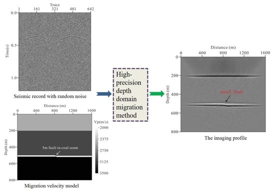
3. Numerical Examples

In this section, a 2D coal-measure small fault model is established for the PSDM test (Figure 1). The model is 1600 m in length and 800 m in depth, and the sizes of the longitudinal and horizontal grids are 5 m. There are four layers in the model: the first layer is mudstone, the second is sandstone, the third is a coal seam, and the fourth is limestone. There is a small fault in the coal seam with a fault distance of 8 m. The specific parameters of each layer are shown in Table 1. The finite difference method was used for synthesizing seismic records. The seismic source is a Ricker wavelet of 80 Hz, and the receiving mode is a full-array reception. A total of 51 shots were simulated, and the shot spacing was 30 m. Each shot had 321 receivers, and the receiver spacing was 5 m. The recording time was 1.2 s, and the sampling interval was 1 ms. The original single-shot seismic record of the 26th shot is shown in Figure 2. The proposed RTM method was used to conduct imaging, and the direct waves were eliminated in the migration process. Figure 3 shows the final imaging results. As can be seen, the reflection interfaces in the model are located at the real position, and accurate imaging results are obtained. In addition, the small fault in the coal seam can be clearly seen on the imaging profile (as denoted by the arrow), which means that it can be effectively identified. Next, we added strong random noise to the seismic records for migration testing. Figure 4 shows the 26th single-shot seismic record with random noise, where the signal-to-noise ratio was poor. Figure 5 shows the imaging results of the noised seismic data using our migration method. The noise had little effect on imaging, and accurate imaging results were also obtained, which could effectively identify the small fault structure in the coal seam (as denoted by the arrow). Through the migration test on the coal-measure small fault model, the precision and efficiency of the proposed migration method in terms of the imaging of coal-measure strata with small faults were verified.
To further verify the imaging precision of our proposed migration method for small fault structures in coal-measure strata, we adjusted the fault distance of the small fault in the coal seam model to 5 m and kept the other model parameters unchanged for the migration test (Figure 6). We performed a forward simulation on the coal seam model using the same parameters. Then, as above, we conducted the reverse time migration of the original seismic data and the high-noise seismic data; the corresponding imaging results are shown in Figure 7 and Figure 8, respectively. As can be seen, precise focus imaging can be realized, and a small fault structure with a fault distance of 5 m in the coal seam model can still be accurately identified on both profiles (as denoted by the arrows). These results further verify the effectiveness of the proposed migration method for precise detection of small faults with a fault distance of 5 m in coal-measures strata.

4. Seismic Data Example of Field Coalfields

To further verify the practicability of our proposed method, the migration of actual 3D seismic data of a coalfield in the northeast of the Ordos Plateau in China was conducted. The surface lithology of the study area greatly varies. The western ridge is a gravel outcrop area, while other areas are mostly covered by Quaternary wind-drift sand and sandy soil with little bedrock outcrop. The shallow-surface seismic and geological conditions in the study area are complex. The main sedimentary strata in the field include the Triassic upper-series Yanchang formation, the Jurassic middle- and lower-series Yan’an formation, the middle-series Zhiluo formation and Anding formation, the Cretaceous lower-series Yijinhuoluo formation, the Quaternary upper Pleistocene Salawusu formation, and the Holocene strata. The main coal seams in the area are deep in the west and shallow in the east, and the development of wrinkles is not obvious. Fault structures are developed in the middle and north of the area, and the fault strike is essentially along the N-shaped direction, which has a certain regularity. The observation system in this coalfield 3D seismic exploration adopted a bundle system of 14 lines and 4 shots, with shooting shots in the middle. Each line had 60 receivers. The receiver distance was 10 m. The distance between the lines was 20 m. The longitudinal offset was 10 m. The longitudinal maximum offset was 300 m, and the transverse maximum offset was 190 m. A total of 1317 shots were acquired. The recording time was 1 s, and the sampling time was 1 ms. The coverage times of the data acquisition are shown in Figure 9, and the original 488th shot gather is shown in Figure 10.
According to the characteristics of 3D seismic data, we adopted fine processing techniques, such as static correction, noise suppression, and deconvolution, to preprocess the original 3D seismic data and conduct migration velocity modeling. Figure 11 shows the prestack 488th shot gather after seismic data processing, and Figure 12 shows the migration velocity model. The 3D RTM method proposed in this study was used to carry out prestack depth migration for the 3D seismic data, and the imaging result is shown in Figure 13. As can be seen, the imaging profile has a high resolution, strong energy, and accurate positioning, and the wave group characteristics of the targeted coal seam are prominent. The imaging depth of the targeted coal seam is well-matched with the depth of the coal seam revealed by the logging interpretation layered data in this area, and the depth error is within 3~5 m. To better display the imaging results, two inline and crossline profiles were extracted, and the imaging results obtained by the proposed migration method were compared with those of the conventional RTM method. Figure 14a,b show two different inline profiles extracted by our migration method, and Figure 14c,d show the two corresponding inline profiles extracted by the conventional RTM method. Figure 15a,b show two different crossline profiles extracted by our migration method, and Figure 15c,d show the two corresponding crossline profiles extracted by the conventional RTM method. It can be seen that both migration methods obtain accurate images. Compared with the conventional RTM results, the image quality is slightly improved using our proposed migration method. Moreover, small fault structures in coal seams can be clearly identified from the imaging profiles, as shown by arrow in Figure 15. Through the migration test of the 3D seismic data of the actual coalfield, the efficiency of the 3D RTM method proposed in this study and its practicability in the accurate exploration of fault structures in coal-measure strata were further verified.

5. Conclusions

Based on the variable-density acoustic equation optimized with a temporal–spatial staggered-grid finite difference forward method and the combination of the normalized cross-correlation imaging condition and the GPU/CPU collaborative parallel processing technology, we proposed an efficient and high-precision 3D RTM method suitable for 3D seismic data in the area of coal mining. Compared with the conventional finite difference method, we solved the difference coefficients based on the optimized inversion algorithm, which can greatly improve the simulation accuracy in the high-frequency band and achieve a high-precision numerical simulation of a seismic wave in the full-frequency band, thus improving the imaging quality. In addition, the GPU/CPU collaborative parallel imaging strategy can effectively improve the computational efficiency of migration. According to the numerical test of seismic migration on the small fault model in coal measures, an accurate focusing imaging for the reflected interface of the model could be obtained, and small faults with fault distances of 5 m and 8 m in the coal seams could be effectively identified. This verified the precision of the proposed migration method and its feasibility in detecting small fault structures in coal measures. Through prestack depth migration for the actual 3D seismic data by our 3D RTM method, the 3D depth-domain imaging profile could be accurately positioned, and the targeted coal seam could be accurately imaged, thus precisely identifying the small fault structures in coal seam, which further verified the effectiveness and practicability of the 3D coalfield RTM method. Our work provides an efficient imaging method for the precise exploration of actual coal-measure strata.

Author Contributions

Conceptualization, J.H.; methodology, J.H. and B.G.; software, Z.L. and B.G.; validation, J.H., G.Z. and Z.L.; formal analysis, Z.L.; investigation, G.Z.; resources, G.Z.; data curation, J.H.; writing—original draft preparation, J.H.; writing—review and editing, J.H.; visualization, Z.L.; supervision, J.H. and B.G.; project administration, J.H. and G.Z.; funding acquisition, G.Z. All authors have read and agreed to the published version of the manuscript.

Funding

This research was funded by the National Natural Science Foundation of China (Grant No. 42174157, 42004093), CAGS Research Fund (Grant No. JKY202216), Enterprise Cooperative Development Project (Grant No. 5600B2021000004, ZY20-XA202-TPGC272, SMDZ(KY)-2020-004, XNS-KYY-JS2021-014, 33550007-20-ZC0613-0088), and the China Geological Survey Project (Grant No. DD20211343).

Data Availability Statement

The data underlying this article will be shared on reasonable request made to the corresponding author.

Acknowledgments

The authors would like to thank Zhiming Ren for his guidance and help with the seismic wavefield forward simulation method.

Conflicts of Interest

The authors declare no conflict of interest.

References

  1. Wang, Y.; Lu, J.; Yu, G. A normal fault in coal seams with drop height less than 3 m can be identified in seismic exploration. J. China Coal Soc. 2010, 35, 629–634. [Google Scholar]
  2. Lambourne, A.N.; Evans, B.J.; Hatherly, P.J. The application of the 3D seismic surveying technique to coal seam imaging: Case histories from the Arckaringa and Sydney basins. Explor. Geophys. 1989, 20, 137–141. [Google Scholar] [CrossRef]
  3. Walton, C.; Evans, B.; Urosevic, M. Imaging coal seam structure using 3-D seismic methods. Explor. Geophys. 2000, 31, 509–514. [Google Scholar] [CrossRef]
  4. Pei, X.D. Signal acquisition method for 3D seismic exploration in high density coal mining area. Arab. J. Geosci. 2020, 13, 712. [Google Scholar] [CrossRef]
  5. Han, J.G.; Wang, Y.; Lu, J. Multi-component Gaussian beam prestack depth migration. J. Geophys. Eng. 2013, 10, 055008. [Google Scholar] [CrossRef]
  6. Han, J.G.; Lü, Q.T.; Gu, B.L.; Yan, J.Y.; Zhang, H. 2D anisotropic multicomponent Gaussian-beam migration under complex surface conditions. Geophysics 2020, 85, S89–S102. [Google Scholar] [CrossRef]
  7. Gu, B.L.; Huang, J.P.; Han, J.G.; Ren, Z.M.; Li, Z.C. Least-squares inversion-based elastic reverse time migration with PP- and PS-angle-domain common-imaging gathers. Geophysics 2021, 86, S29–S44. [Google Scholar] [CrossRef]
  8. Hu, H.; Xiang, S. Application of pre-stack depth migration technique in salt bed. Petrol. Explor. Dev. 2006, 33, 194–197. [Google Scholar]
  9. Liu, D.J.; Yin, X.Y. A method of Fourier finite-difference preserved-amplitude prestack depth migration. Chin. J. Geophys. 2007, 50, 268–276. [Google Scholar] [CrossRef]
  10. Yang, J.D.; Huang, J.P.; Wang, X.; Li, Z.C. An amplitude-preserved adaptive focused beam seismic migration method. Petrol. Sci. 2015, 12, 417–427. [Google Scholar] [CrossRef] [Green Version]
  11. Gu, B.L.; Han, J.G.; Ren, Z.M.; Li, Z.C. 2D least-squares elastic reverse time migration of multicomponent seismic data. Geophysics 2019, 84, S523–S538. [Google Scholar] [CrossRef]
  12. Chang, W.F.; McMechan, G.A. Reverse-time migration of offset vertical seismic profiling data using the excitation-time imaging condition. Geophysics 1986, 51, 67–84. [Google Scholar] [CrossRef]
  13. Symes, W.W. Reverse time migration with optimal checkpointing. Geophysics 2007, 72, SM213–SM221. [Google Scholar] [CrossRef] [Green Version]
  14. Shragge, J. Reverse time migration from topography. Geophysics 2014, 79, S141–S152. [Google Scholar] [CrossRef]
  15. Nguyen, B.D.; McMechan, G.A. Excitation amplitude imaging condition for prestack reverse-time migration. Geophysics 2013, 78, S37–S46. [Google Scholar] [CrossRef]
  16. Nguyen, B.D.; McMechan, G.A. Five ways to avoid storing source wavefield snapshots in 2D elastic prestack reverse time migration. Geophysics 2015, 80, S1–S18. [Google Scholar] [CrossRef]
  17. Liu, Q.C.; Zhang, J.F.; Zhang, H. Eliminating the redundant source effects from the cross-correlation reverse-time migration using a modified stabilized division. Comput. Geosci. 2016, 92, 49–57. [Google Scholar] [CrossRef]
  18. Liu, G.F.; Liu, Y.N.; Ren, L.; Meng, X.H. 3D seismic reverse time migration on GPGPU. Comput. Geosci. 2013, 59, 17–23. [Google Scholar] [CrossRef]
  19. Du, Q.; Gong, X.; Zhang, M.; Zhu, Y.; Fang, G. 3D PS-wave imaging with elastic reverse-time migration. Geophysics 2014, 79, S174–S184. [Google Scholar] [CrossRef]
  20. Rocha, D.; Sava, P.; Guitton, A. 3D acoustic least-squares reverse time migration using the energy norm. Geophysics 2018, 83, S261–S270. [Google Scholar] [CrossRef]
  21. Gu, B.L.; Ren, Z.M.; Li, Q.Q.; Han, J.G.; Li, Z.C. An application of vector wavefield decomposition to 3D elastic reverse time migration and field data test. Comput. Geosci. 2019, 131, 112–131. [Google Scholar] [CrossRef]
  22. Ren, Z.M.; Bao, Q.Z.; Xu, S.G. Memory-efficient source wavefield reconstruction and its application to 3D reverse time migration. Geophysics 2022, 87, S21–S34. [Google Scholar] [CrossRef]
  23. Chang, W.; McMechan, G.A. Elastic reverse-time migration. Geophysics 1987, 52, 1367–1375. [Google Scholar] [CrossRef]
  24. Yan, J.; Sava, P. Isotropic angle-domain elastic reverse-time migration. Geophysics 2008, 73, S229–S239. [Google Scholar] [CrossRef] [Green Version]
  25. Du, Q.Z.; Zhu, Y.T.; Ba, J. Polarity reversal correction for elastic reverse time migration. Geophysics 2012, 77, S31–S41. [Google Scholar] [CrossRef]
  26. Du, Q.Z.; Guo, C.F.; Zhao, Q.; Gong, X.F.; Wang, C.X.; Li, X.Y. Vector-based elastic reverse time migration based on scalar imaging condition. Geophysics 2017, 82, S111–S127. [Google Scholar] [CrossRef]
  27. Yong, P.; Huang, J.P.; Li, Z.C.; Liao, W.Y.; Qu, L.P.; Li, Q.Y.; Yuan, M.L. Elastic wave reverse-time migration based on decoupled elastic-wave equations and inner-product imaging condition. J. Geophys. Eng. 2016, 13, 953–963. [Google Scholar] [CrossRef]
  28. Ren, Z.M.; Liu, Y.; Sen, M.K. Least-squares reverse time migration in elastic media. Geophys. J. Int. 2017, 208, 1103–1125. [Google Scholar] [CrossRef]
  29. Ren, Z.; Li, Z. Imaging of elastic seismic data by least-squares reverse time migration with weighted L2-norm multiplicative and modified total-variation regularizations. Geophys. Prospect. 2020, 68, 411–430. [Google Scholar] [CrossRef]
  30. Fowler, P.J.; Du, X.; Fletcher, R.P. Couple equations for reverse time migration in transversely isotropic media. Geophysics 2010, 75, S11–S22. [Google Scholar] [CrossRef]
  31. Li, C.; Liu, G.F.; Li, Y.H. A practical implementation of 3D TTI reverse time migration with multi-GPUs. Comput. Geosci. 2017, 102, 68–78. [Google Scholar] [CrossRef]
  32. Yang, J.; Zhang, H.; Zhao, Y.; Zhu, H. Elastic wavefield separation in anisotropic media based on eigenform analysis and its application in reverse-time migration. Geophys. J. Int. 2019, 217, 1290–1313. [Google Scholar] [CrossRef]
  33. Yang, J.; Zhu, H.; McMechan, G.; Zhang, H.; Zhao, Y. Elastic least-squares reverse time migration in vertical transverse isotropic media. Geophysics 2019, 84, S539–S553. [Google Scholar] [CrossRef]
  34. Gu, B.L.; Li, Z.C.; Han, J.G. A wavefield-separation-based elastic least-squares reverse time migration. Geophysics 2018, 83, S279–S297. [Google Scholar] [CrossRef]
  35. Virieux, J. P-SV wave propagation in heterogeneous media: Velocity-stress finite difference method. Geophysics 1986, 51, 889–901. [Google Scholar] [CrossRef]
  36. Graves, R.W. Simulating seismic wave progation in 3D elastic media using staggered-grid finite difference. Bull. Seismol. Soc. Am. 1996, 86, 1091–1106. [Google Scholar]
  37. Appelö, D.; Petersson, N.A. A stable finite difference method for the elastic wave equation on complex geometries with free surfaces. Commun. Comput. Phys. 2009, 5, 84–107. [Google Scholar]
  38. Ren, Z.M.; Li, Z.C.; Liu, Y.; Sen, M.K. Modeling of the acoustic wave equation by staggered-grid finite-difference schemes with high-order temporal and spatial accuracy. Bull. Seismol. Soc. Am. 2017, 107, 2160–2182. [Google Scholar] [CrossRef]
  39. Ren, Z.M.; Li, Z.C. High-order temporal and implicit spatial staggered-grid finite-difference operators for modelling seismic wave propagation. Geophys. J. Int. 2019, 217, 844–865. [Google Scholar] [CrossRef]
Figure 1. Coal-measure small fault model with a fault distance of 8 m. The first layer of the model is mudstone, and the second is sandstone. The third layer is a coal seam, which has 8 m small fault. The fourth layer is limestone.
Remotesensing 14 02850 g001
Figure 2. The 26th original single-shot seismic record, which has 321 receivers, and the recording time is 1.2 s.
Remotesensing 14 02850 g002
Figure 3. The imaging result of the original seismic data for coal-measure 8 m fault model. The accurate focused imaging of the 8 m small fault in coal seam was obtained, as denoted by the black arrow.
Remotesensing 14 02850 g003
Figure 4. The 26th single-shot seismic record with random noise, where it has high noise.
Remotesensing 14 02850 g004
Figure 5. The imaging result of the noised seismic data, where the small fault structure in coal seam can also be effectively identified, as denoted by the black arrow.
Remotesensing 14 02850 g005
Figure 6. Coal-measure small fault model with a fault distance of 5 m. The fault distance of the small fault in the coal seam is adjusted to 5 m, and the other model parameters are the same as those of the above model.
Remotesensing 14 02850 g006
Figure 7. The imaging result of the original seismic data for coal-measure 5 m fault model. The 5 m small fault in the coal seam is accurately identified, as denoted by the black arrow.
Remotesensing 14 02850 g007
Figure 8. The imaging result of the high noised seismic data, where the small fault structure in coal seam can still be accurately identified, as denoted by the black arrow.
Remotesensing 14 02850 g008
Figure 9. Schematic diagram of coverage times of the seismic data acquisition. The full coverage is 24, and the maximum coverage is less than 60 times.
Remotesensing 14 02850 g009
Figure 10. The original 488th shot gather. There are obvious static correction problems in the seismic record as well as serious noise disturbances.
Remotesensing 14 02850 g010
Figure 11. The prestack 488th shot gather after seismic data processing. The distortion of the reflection event is well-corrected, the noise is effectively suppressed, and the signal-to-noise ratio is significantly improved.
Remotesensing 14 02850 g011
Figure 12. The migration velocity model.
Remotesensing 14 02850 g012
Figure 13. The imaging result of 3D seismic data of the actual coalfield using our 3D RTM method. The target coal seam is well-imaged.
Remotesensing 14 02850 g013
Figure 14. The extracted two different inline profiles. The imaging profiles of (a) inline70 and (b) inline110 obtained using our proposed migration method. The imaging profiles of (c) inline70 and (d) inline110 obtained using the conventional RTM method.
Remotesensing 14 02850 g014
Figure 15. The extracted two different crossline profiles. The imaging profiles of (a) crossline280 and (b) crossline340 obtained using our proposed migration method. The imaging profiles of (c) crossline280 and (d) crossline340 obtained using the conventional RTM method. The red arrows indicate the small fault structures in coal seams.
Remotesensing 14 02850 g015aRemotesensing 14 02850 g015b
Table 1. Parameters of coal-measure fault model.
LayerLithology v P   ( m / s ) v S   ( m / s ) ρ (g/cm3) Layer Thickness (m)
1mudstone250014501.8200
2sandstone310017802.2300
3coal seam200011501.415
4limestone350020202.3285
Publisher’s Note: MDPI stays neutral with regard to jurisdictional claims in published maps and institutional affiliations.

