
Research on Service Value and Adaptability Zoning of Grassland Ecosystem in Ethiopia

Abstract
:
1. Introduction
2. Materials and Methods
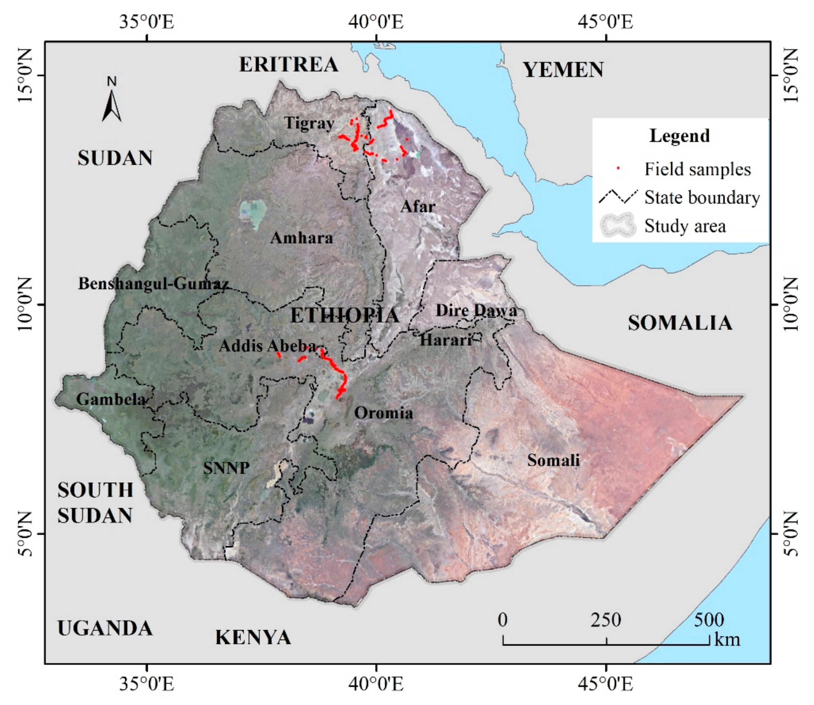
2.1. Study Area
2.2. Datasets
2.2.1. Sample Points of Grassland
2.2.2. Remote Sensing and Related Products
2.2.3. Others
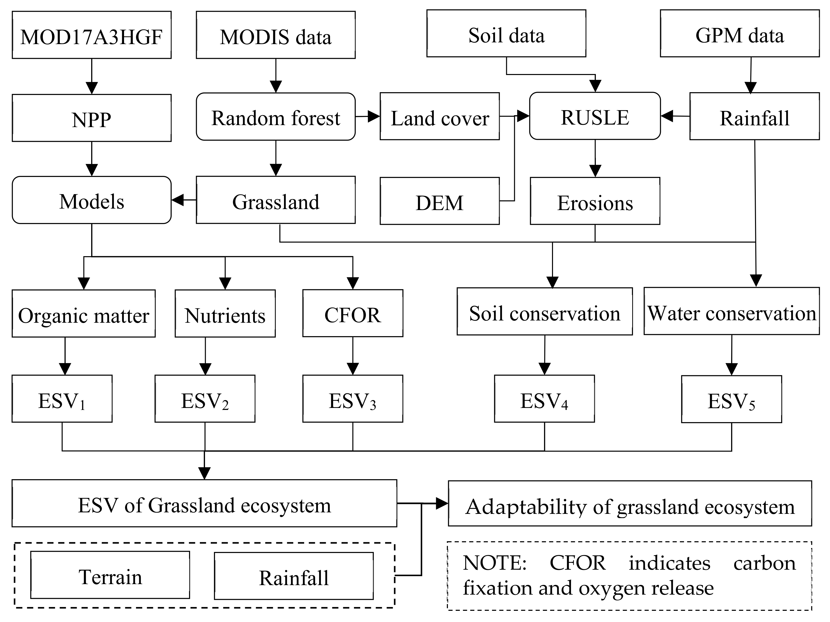
2.3. Methodology
2.3.1. Extraction of Grass Coverage
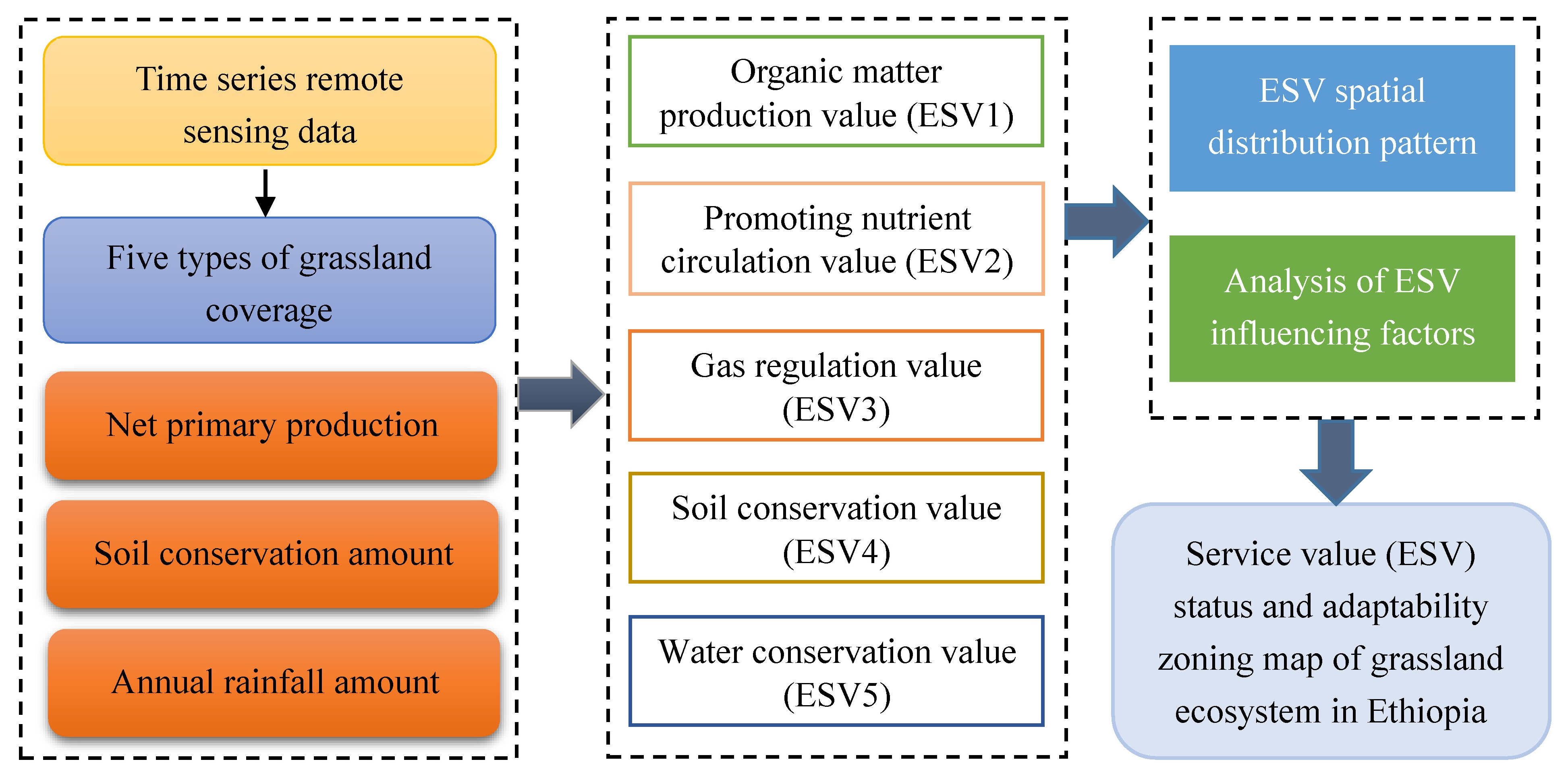
2.3.2. ESV Calculation of Grassland
- (1)
- Organic matter production
- (2)
- Promoting nutrient circulation
- (3)
- Gas regulation
- (4)
- Soil conservation
- (5)
- Water regulation
- (6)
- Total ESV of grassland ecosystem
2.3.3. Regionalization of Grassland Ecosystem
- (1)
- Analysis of ESV distribution characteristics
- (2)
- Adaptability zoning of grassland ecosystem
3. Results and Analysis
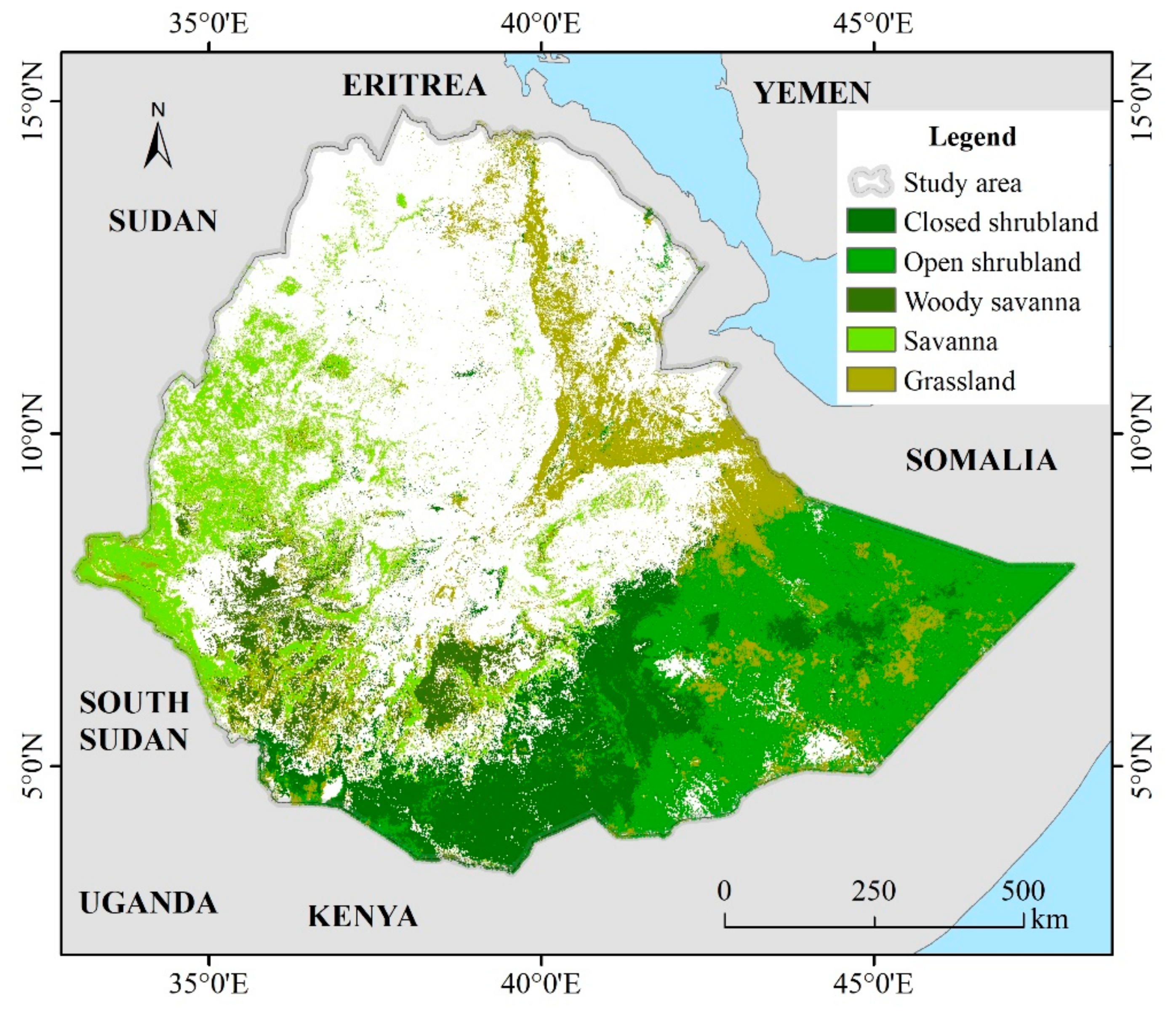
3.1. Grass Coverage of Ethiopia
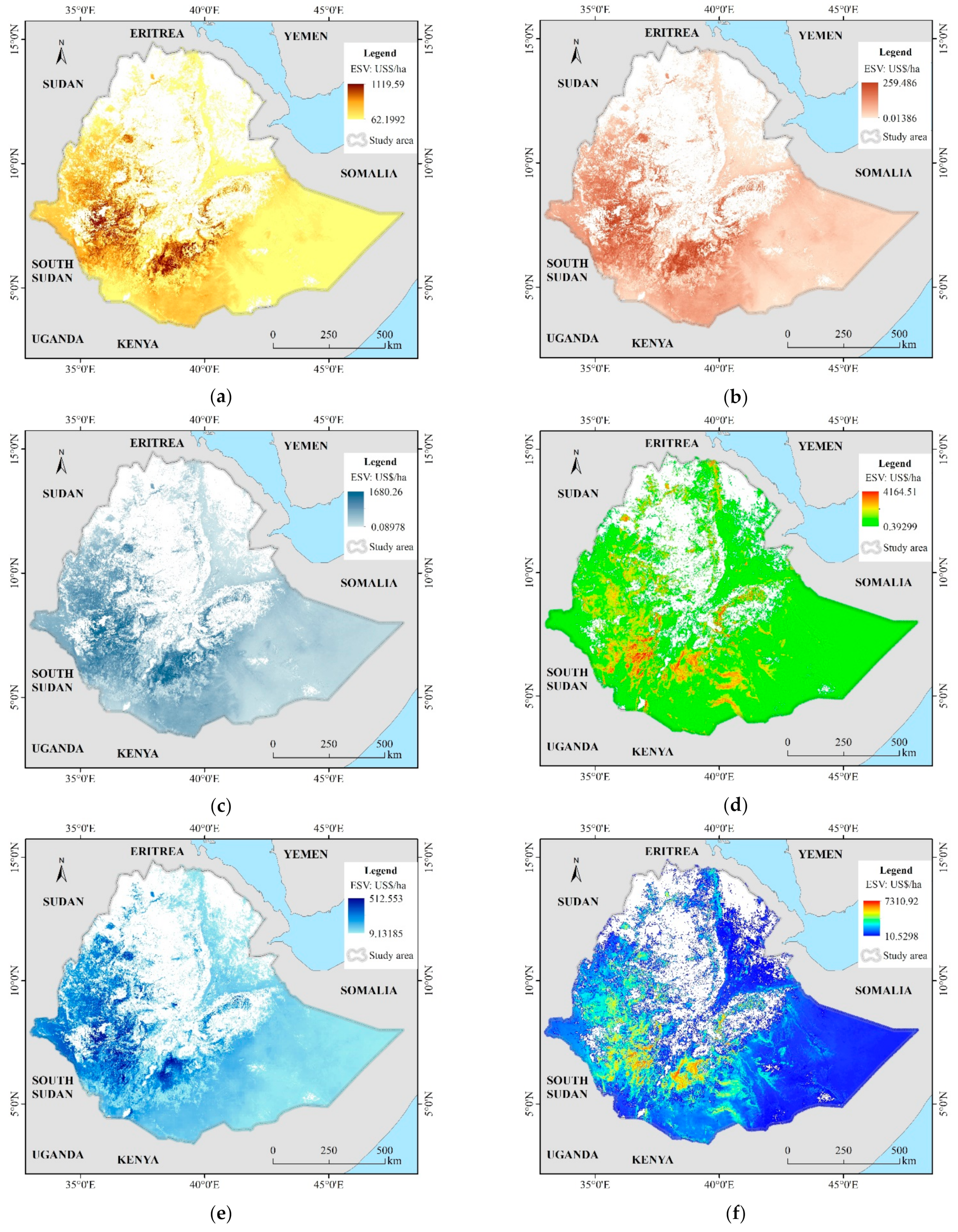
3.2. ESV of Grassland Ecosystem
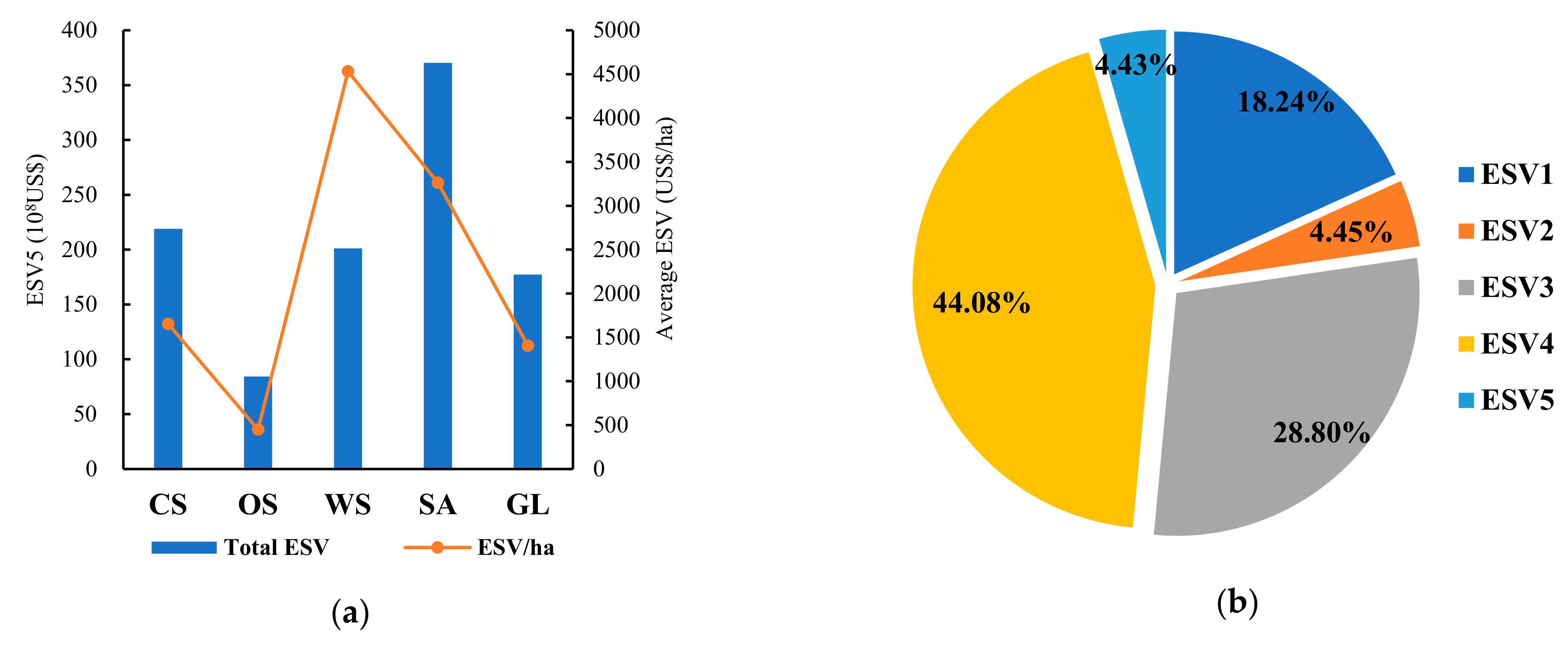
3.2.1. Differences in Grassland Types and Ecosystem Service Functions
3.2.2. Distribution of Grassland ESV in Various States
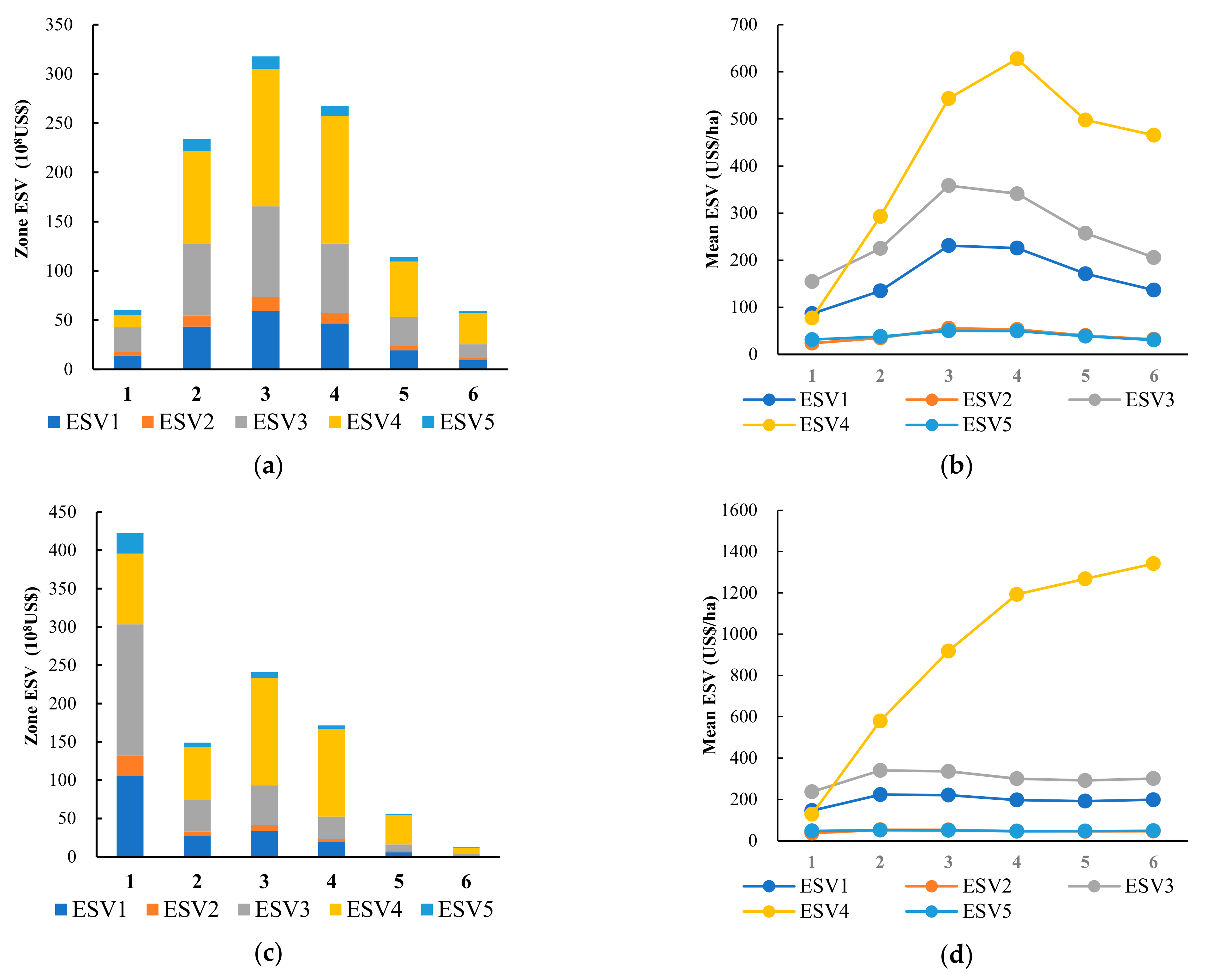
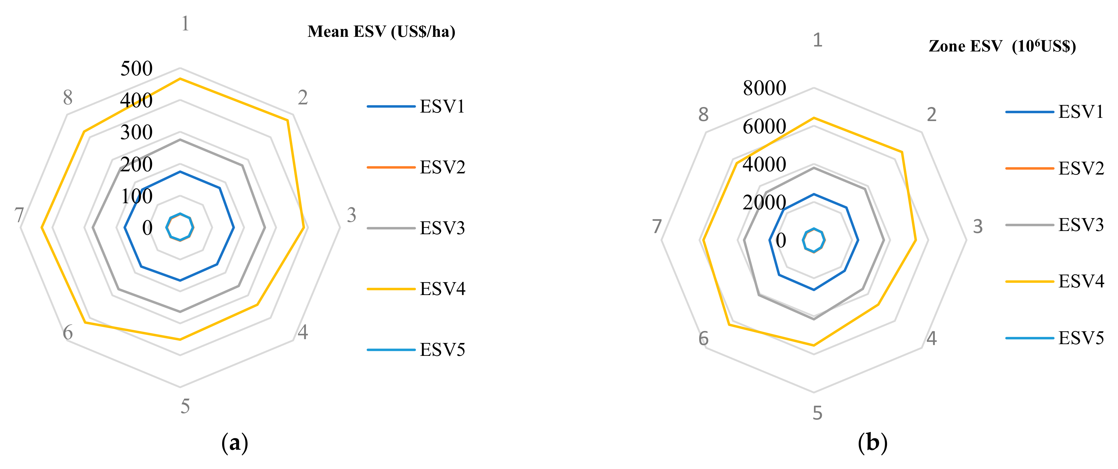
3.2.3. Influence of Topography on ESV
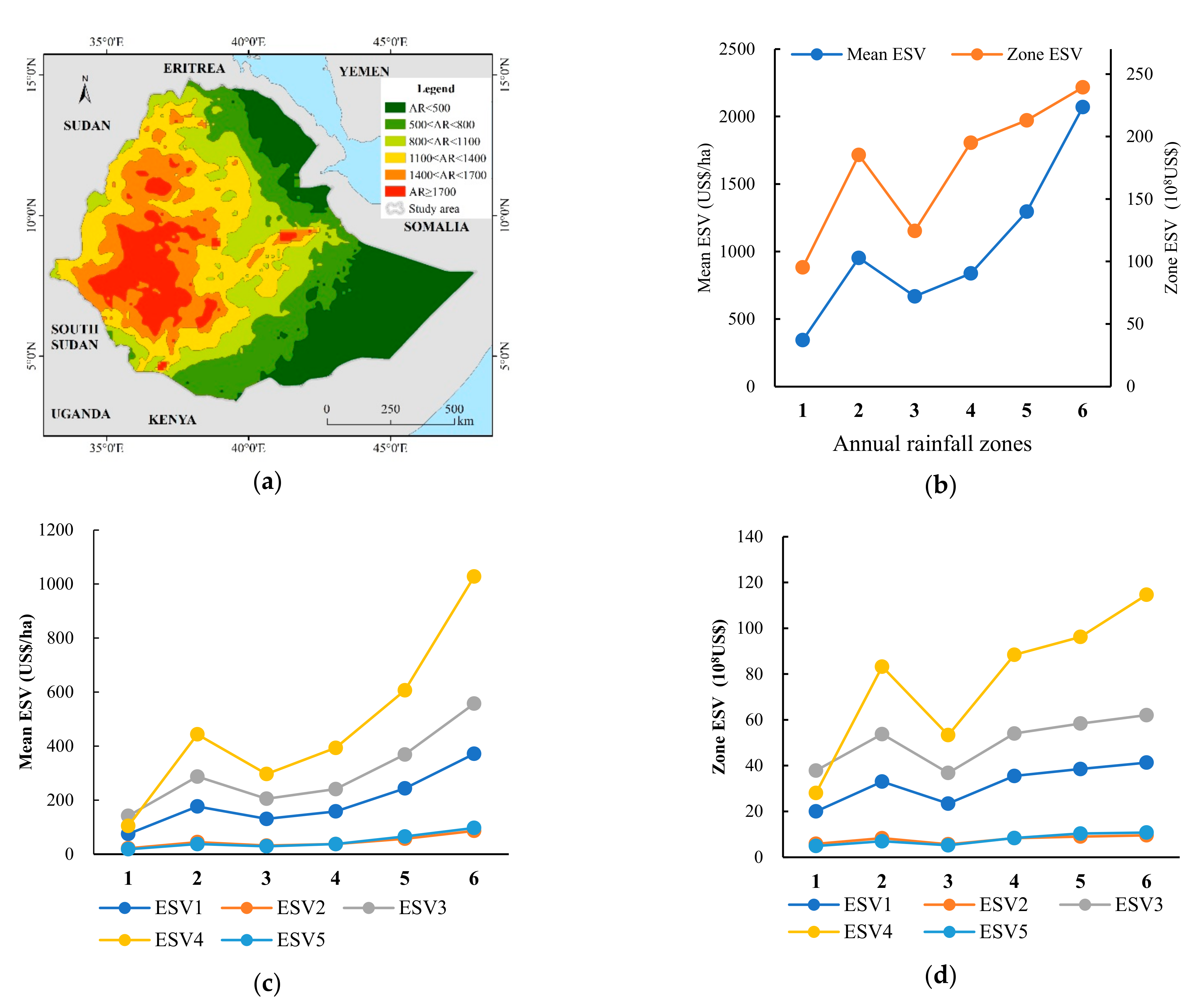
3.2.4. Relationship between ESV and Rainfall
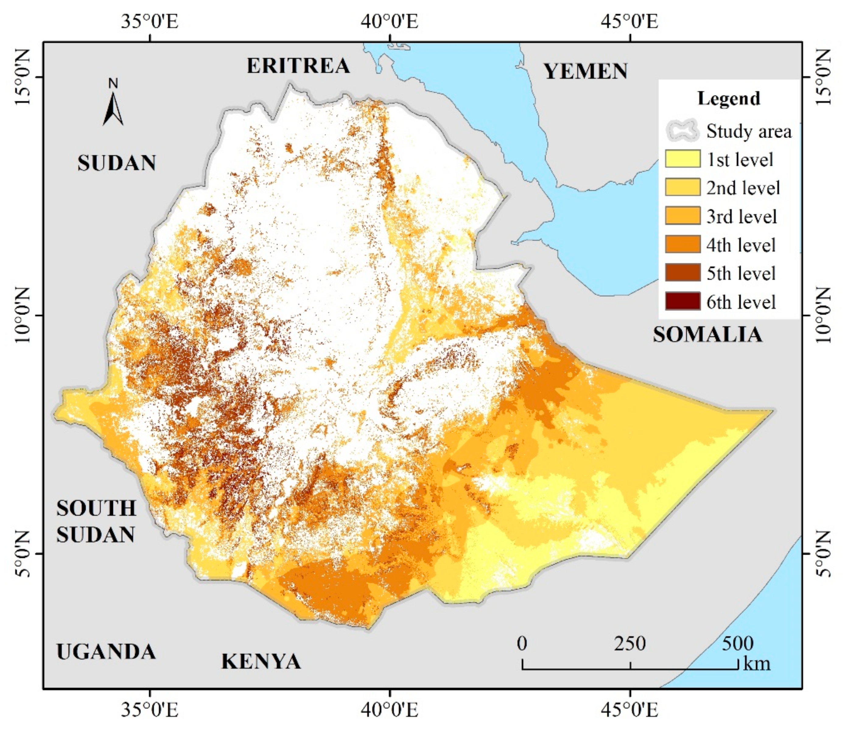
3.3. Adaptability Zoning of Grassland Ecosystem
4. Discussion
4.1. Datasets and Classification Methods
4.2. Research on ESV
4.3. Guiding Significance of ESV
5. Conclusions
Author Contributions
Funding
Data Availability Statement
Acknowledgments
Conflicts of Interest
References
- Leemans, R.; de Groot, R.S. Millennium Ecosystem Assessment: Ecosystems and Human Wellbeing: A Framework for Assessment; World Resources Institute: Washington, DC, USA, 2003. [Google Scholar]
- Gashaw, T.; Tulu, T.; Argaw, M.; Worqlul, A.W.; Tolessa, T.; Kindu, M. Estimating the impacts of land use/land cover changes on Ecosystem Service Values: The case of the Andassa watershed in the Upper Blue Nile basin of Ethiopia. Ecosyst. Serv. 2018, 31, 219–228. [Google Scholar] [CrossRef]
- Cao, Y.; Cao, Y.; Li, G.; Tian, Y.; Fang, X.; Li, Y.; Tan, Y. Linking ecosystem services trade-offs, bundles and hotspot identification with cropland management in the coastal Hangzhou Bay area of China. Land Use Policy 2020, 97, 104689. [Google Scholar] [CrossRef]
- Li, R.; Shi, Y.; Feng, C.-C.; Guo, L. The spatial relationship between ecosystem service scarcity value and urbanization from the perspective of heterogeneity in typical arid and semiarid regions of China. Ecol. Indic. 2021, 132, 108299. [Google Scholar] [CrossRef]
- Yang, Q.; Liu, G.; Giannetti, B.F.; Agostinho, F.; Almeida, C.M.V.B.; Casazza, M. Emergy-based ecosystem services valuation and classification management applied to China’s grasslands. Ecosyst. Serv. 2020, 42, 101073. [Google Scholar] [CrossRef]
- Costanza, R.; d’Arge, R.; de Groot, R.; Farber, S.; Grasso, M.; Hannon, B.; Limburg, K.; Naeem, S.; O’Neill, R.V.; Paruelo, J.; et al. The value of the world’s ecosystem services and natural capital. Nature 1997, 387, 253–260. [Google Scholar] [CrossRef]
- Anaya-Romero, M.; Muñoz-Rojas, M.; Ibáñez, B.; Marañón, T. Evaluation of forest ecosystem services in Mediterranean areas. A regional case study in South Spain. Ecosyst. Serv. 2016, 20, 82–90. [Google Scholar] [CrossRef]
- Kindu, M.; Schneider, T.; Teketay, D.; Knoke, T. Changes of ecosystem service values in response to land use/land cover dynamics in Munessa-Shashemene landscape of the Ethiopian highlands. Sci. Total Environ. 2016, 547, 137–147. [Google Scholar] [CrossRef] [PubMed]
- Costanza, R.; de Groot, R.; Braat, L.; Kubiszewski, I.; Fioramonti, L.; Sutton, P.; Farber, S.; Grasso, M. Twenty years of ecosystem services: How far have we come and how far do we still need to go? Ecosyst. Serv. 2017, 28, 1–16. [Google Scholar] [CrossRef]
- Costanza, R.; Kubiszewski, I. The authorship structure of “ecosystem services” as a transdisciplinary field of scholarship. Ecosyst. Serv. 2012, 1, 16–25. [Google Scholar] [CrossRef] [Green Version]
- Braat, L.; de Groot, R. The ecosystem services agenda: Bridging the worlds of natural science and economics, conservation and development, and public and private policy. Ecosyst. Serv. 2012, 1, 4–15. [Google Scholar] [CrossRef] [Green Version]
- Costanza, R.; de Groot, R.; Sutton, P.; van der Ploeg, S.; Anderson, S.J.; Kubiszewski, I.; Farber, S.; Turner, R.K. Changes in the global value of ecosystem services. Glob. Environ. Chang. 2014, 26, 152–158. [Google Scholar] [CrossRef]
- Hu, H.; Liu, W.; Cao, M. Impact of land use and land cover changes on ecosystem services in Menglun, Xishuangbanna, Southwest China. Environ. Monit. Assess. 2008, 146, 147–156. [Google Scholar] [CrossRef] [PubMed]
- Liu, S.; Costanza, R.; Troy, A.; D’Aagostino, J.; Mates, W. Valuing New Jersey’s ecosystem services and natural capital: A spatially explicit benefit transfer approach. Environ. Manag. 2010, 45, 1271–1285. [Google Scholar] [CrossRef] [PubMed]
- Frélichová, J.; Vačkář, D.; Pártl, A.; Loučková, B.; Harmáčková, Z.V.; Lorencová, E. Integrated assessment of ecosystem services in the Czech Republic. Ecosyst. Serv. 2014, 8, 110–117. [Google Scholar] [CrossRef]
- Shi, Y.; Feng, C.; Yu, Q.; Guo, L. Integrating supply and demand factors for estimating ecosystem services scarcity value and its response to urbanization in typical mountainous and hilly regions of south China. Sci. Total Environ. 2021, 796, 149032. [Google Scholar] [CrossRef]
- Schägner, J.P.; Brander, L.; Maes, J.; Hartje, V. Mapping ecosystem services’ values: Current practice and future prospects. Ecosyst. Serv. 2013, 4, 33–46. [Google Scholar] [CrossRef] [Green Version]
- Bateman, I.J.; Harwood, A.R.; Mace, G.M.; Watson, R.T.; Abson, D.J.; Andrews, B.; Binner, A.; Crowe, A.; Day, B.H.; Dugdale, S.; et al. Bringing ecosystem services into economic decision-making: Land use in the United Kingdom. Science 2013, 341, 45–50. [Google Scholar] [CrossRef] [PubMed]
- Morshed, S.R.; Fattah, M.A.; Haque, M.N.; Morshed, S.Y. Future ecosystem service value modeling with land cover dynamics by using machine learning based Artificial Neural Network model for Jashore city, Bangladesh. Phys. Chem. Earth Parts A B C 2022, 126, 103021. [Google Scholar] [CrossRef]
- MEA (Millennium Ecosystem Assessment). Ecosystems and Human Wellbeing: Biodiversity Synthesis; World Resources Institute: Washington, DC, USA, 2005. [Google Scholar]
- Degefu, M.A.; Argaw, M.; Feyisa, G.L.; Degefa, S. Dynamics of urban landscape nexus spatial dependence of ecosystem services in rapid agglomerate cities of Ethiopia. Sci. Total Environ. 2021, 798, 149192. [Google Scholar] [CrossRef]
- Li, R.; Dong, M.; Cui, J.; Zhang, L.; Cui, Q.; He, W. Quantification of the impact of land-use changes on ecosystem services: A case study in Pingbian County, China. Environ. Monit. Assess. 2007, 128, 503–510. [Google Scholar] [CrossRef]
- Tolessa, T.; Senbeta, F.; Kidane, M. The impact of land use/land cover change on ecosystem services in the central highlands of Ethiopia. Ecosyst. Serv. 2017, 23, 47–54. [Google Scholar] [CrossRef]
- Wang, Z.; Zhang, B.; Zhang, S.; Li, X.; Liu, D.; Song, K.; Li, J.; Li, F.; Duan, H. Changes of land use and of ecosystem service values in Sanjiang Plain, Northeast China. Environ. Monit. Assess. 2006, 112, 69–91. [Google Scholar] [CrossRef] [PubMed]
- Limburg, K.E.; O’Neill, R.V.; Costanza, R.; Farber, S. Complex systems and valuation. Ecol. Econ. 2002, 41, 409–420. [Google Scholar] [CrossRef]
- Hein, L.; van Koppen, K.; de Groot, R.S.; van Ierland, E.C. Spatial scales, stakeholders and the valuation of ecosystem services. Ecol. Econ. 2006, 57, 209–228. [Google Scholar] [CrossRef]
- Maes, J.; Egoh, B.; Willemen, L.; Liquete, C.; Vihervaara, P.; Schägner, J.P.; Grizzetti, B.; Drakou, E.G.; La Notte, A.; Zulian, G.; et al. Mapping ecosystem services for policy support and decision making in the European Union. Ecosyst. Serv. 2012, 1, 31–39. [Google Scholar] [CrossRef]
- Wang, X.; Dong, X.; Liu, H.; Wei, H.; Fan, W.; Lu, N.; Xu, Z.; Ren, J.; Xing, K. Linking land use change, ecosystem services and human well-being: A case study of the Manas River Basin of Xinjiang, China. Ecosyst. Serv. 2017, 27, 113–123. [Google Scholar] [CrossRef]
- Van der Ploeg, S.; de Groot, D. The TEEB Valuation Database–A Searchable Database of 1310 Estimates of Monetary Values of Ecosystem Services; Foundation for Sustainable Development: Wageningen, The Netherlands, 2010. [Google Scholar]
- De Groot, R.; Brander, L.; van der Ploeg, S.; Costanza, R.; Bernard, F.; Braat, L.; Christie, M.; Crossman, N.; Ghermandi, A.; Hein, L.; et al. Global estimates of the value of ecosystems and their services in monetary units. Ecosyst. Serv. 2012, 1, 50–61. [Google Scholar] [CrossRef]
- Li, X.; Lyu, X.; Dou, H.; Dang, D.; Li, S.; Li, X.; Li, M.; Xuan, X. Strengthening grazing pressure management to improve grassland ecosystem services. Glob. Ecol. Conserv. 2021, 31, e01782. [Google Scholar] [CrossRef]
- Knoke, T.; Steinbeis, O.-E.; Bösch, M.; Román-Cuesta, R.M.; Burkhardt, T. Cost-effective compensation to avoid carbon emissions from forest loss: An approach to consider price–quantity effects and risk-aversion. Ecolog. Econ. 2011, 70, 1139–1153. [Google Scholar] [CrossRef]
- Kubiszewski, I.; Costanza, R.; Dorji, L.; Thoennes, P.; Tshering, K. An initial estimate of the value of ecosystem services in Bhutan. Ecosyst. Serv. 2013, 3, e11–e21. [Google Scholar] [CrossRef]
- De Groot, R.S.; Wilson, M.A.; Boumans, R.M. A typology for the classification, description and valuation of ecosystem functions, goods and services. Ecol. Econ. 2002, 41, 393–408. [Google Scholar] [CrossRef] [Green Version]
- Styers, D.M.; Chappelka, A.H.; Marzen, L.J.; Somers, G.L. Developing a land-cover classification to select indicators of forest ecosystem health in a rapidly urbanizing landscape. Landsc. Urban Plan. 2010, 94, 158–165. [Google Scholar] [CrossRef]
- Zhang, X.; Qiu, F.; Qin, F. Identification and mapping of winter wheat by integrating temporal change information and Kullback–Leibler divergence. Int. J. Appl. Earth Obs. Geoinf. 2019, 76, 26–39. [Google Scholar] [CrossRef]
- Wu, M.; Huang, W.; Niu, Z.; Wang, Y.; Wang, C.; Li, W.; Hao, P.; Yu, B. Fine crop mapping by combining high spectral and high spatial resolution remote sensing data in complex heterogeneous areas. Comput. Electron. Agric. 2017, 139, 1–9. [Google Scholar] [CrossRef]
- Qiu, B.; Luo, Y.; Tang, Z.; Chen, C.; Lu, D.; Huang, H.; Chen, Y.; Chen, N.; Xu, W. Winter wheat mapping combining variations before and after estimated heading dates. ISPRS J. Photogramm. Remote Sens. 2017, 123, 35–46. [Google Scholar] [CrossRef]
- Wong, C.Y.S.; Young, D.J.N.; Latimer, A.M.; Buckley, T.N.; Magney, T.S. Importance of the legacy effect for assessing spatiotemporal correspondence between interannual tree-ring width and remote sensing products in the Sierra Nevada. Remote Sens. Environ. 2021, 265, 112635. [Google Scholar] [CrossRef]
- Nabil, M.; Zhang, M.; Bofana, J.; Wu, B.; Stein, A.; Dong, T.; Zeng, H.; Shang, J. Assessing factors impacting the spatial discrepancy of remote sensing based cropland products: A case study in Africa. Int. J. Appl. Earth Obs. Geoinf. 2020, 85, 102010. [Google Scholar] [CrossRef]
- Shiferaw, H.; Bewket, W.; Alamirew, T.; Zeleke, G.; Teketay, D.; Bekele, K.; Schaffner, U.; Eckert, S. Implications of land use/land cover dynamics and Prosopis invasion on ecosystem service values in Afar Region, Ethiopia. Sci. Total Environ. 2019, 675, 354–366. [Google Scholar] [CrossRef]
- Yuan, M.; Lo, S. Ecosystem services and sustainable development: Perspectives from the food-energy-water Nexus. Ecosyst. Serv. 2020, 46, 101217. [Google Scholar] [CrossRef]
- Wu, B.; Tian, Y.; Li, Q. GVG, a Crop Type Proportion Sampling Instrument. J. Remote Sens. 2004, 8, 570–580. [Google Scholar] [CrossRef]
- NASA. Echo. Available online: http://reverb.echo.nasa.gov/ (accessed on 20 September 2021).
- Gandhi, G.M.; Parthiban, S.; Thummalu, N.; Christy, A. NDVI: Vegetation change detection using remote sensing and GIS—A case study of Vellore District. Procedia Comput. Sci. 2015, 57, 1199–1210. [Google Scholar] [CrossRef] [Green Version]
- Zhang, X.; Liu, J.; Qin, Z.; Qin, F. Winter wheat identification by integrating spectral and temporal information derived from multi-resolution remote sensing data. J. Integr. Agric. 2019, 18, 2628–2643. [Google Scholar] [CrossRef]
- NASA. Your Source for Level-1 and Atmospheric Data. Available online: https://ladsweb.modaps.eosdis.nasa.gov/ (accessed on 20 September 2021).
- Fischer, G.; Nachtergaele, F.; Prieler, S.; van Velthuizen, H.T.; Verelst, L.; Wiberg, D. Global Agro-Ecological Zones Assessment for Agriculture (GAEZ 2008); IIASA: Laxenburg, Austria; FAO: Rome, Italy, 2008. [Google Scholar]
- NASA. Global Precipitation Measurement. Available online: https://gpm.nasa.gov/ (accessed on 20 September 2021).
- Mohana, R.M.; Reddy, C.K.K.; Anisha, P.R.; Murthy, B.V.R. Random forest algorithms for the classification of tree-based ensemble. Mater. Today Proc. 2021, in press. [Google Scholar] [CrossRef]
- Tripathi, A.; Goswami, T.; Trivedi, S.K.; Sharma, R.D. A multi class random forest (MCRF) model for classification of small plant peptides. Int. J. Inf. Manag. Data Insights 2021, 1, 100029. [Google Scholar] [CrossRef]
- Zhao, Y.; Zhu, W.; Wei, P.; Fang, P.; Zhang, X.; Yan, N.; Liu, W.; Zhao, H.; Wu, Q. Classification of Zambian grasslands using random forest feature importance selection during the optimal phenological period. Ecol. Indic. 2022, 135, 108529. [Google Scholar] [CrossRef]
- Fang, P.; Yan, N.; Wei, P.; Zhao, Y.; Zhang, X. Aboveground Biomass Mapping of Crops Supported by Improved CASA Model and Sentinel-2 Multispectral Imagery. Remote Sens. 2021, 13, 2755. [Google Scholar] [CrossRef]
- Liu, Y.; Ren, H.; Zhou, R.; Basang, C.; Zhang, W.; Zhang, Z.; Wen, Z. Estimation and dynamic analysis of the service value of grassland ecosystem in China. Acta Agrestia Sin. 2021, 29, 1522–1532. [Google Scholar]
- Zhang, L.; Fan, J.; Zhang, W.; Zhong, H. Stoichiometry of Leaf Nitrogen and Phosphorus in Plants in Grasslands in Inner Mongolia. Chin. J. Grassl. 2014, 36, 43–48. [Google Scholar]
- Lou, P.; Fu, B.; Liu, H.; Gao, E.; Fan, D.; Tang, T.; Lin, X. Dynamic evaluation of grassland ecosystem services in Xilingol League. Acta Ecol. Sin. 2019, 39, 3837–3849. [Google Scholar]
- Zhang, T.; Cao, G.; Cao, S.; Zhang, X.; Zhang, J.; Han, G. Dynamic assessment of the value of vegetation carbon fixation and oxygen release services in Qinghai Lake basin. Acta Ecol. Sin. 2017, 37, 79–84. [Google Scholar] [CrossRef]
- Fenta, A.A.; Yasuda, H.; Shimizu, K.; Haregeweyn, N.; Negussie, A. Dynamics of Soil Erosion as Influenced by Watershed Management Practices: A Case Study of the Agula Watershed in the Semi-Arid Highlands of Northern Ethiopia. Environ. Manag. 2016, 58, 889–905. [Google Scholar] [CrossRef]
- Getnet, T.; Mulu, A. Assessment of soil erosion rate and hotspot areas using RUSLE and multi-criteria evaluation technique at Jedeb watershed, Upper Blue Nile, Amhara Region, Ethiopia. Environ. Chall. 2021, 4, 100174. [Google Scholar] [CrossRef]
- Jiang, H.; Wu, W.; Wang, J.; Yang, W.; Gao, Y.; Duan, Y.; Ma, G.; Wu, C.; Shao, J. Mapping global value of terrestrial ecosystem services by countries. Ecosyst. Serv. 2021, 52, 101361. [Google Scholar] [CrossRef]
- Ouyang, Z.; Wang, X.; Miao, H. A primary study on Chinese terrestrial ecosystem services and their ecological-economic values. Acta Ecol. Sin. 1999, 19, 607–613. [Google Scholar]
- Li, L.; Tang, H.; Lei, J.; Song, X. Spatial autocorrelation in land use type and ecosystem service value in Hainan Tropical Rain Forest National Park. Ecol. Indic. 2022, 137, 108727. [Google Scholar] [CrossRef]
- Wang, A.; Liao, X.; Tong, Z.; Du, W.; Zhang, J.; Liu, X.; Liu, M. Spatial-temporal dynamic evaluation of the ecosystem service value from the perspective of “production-living-ecological” spaces: A case study in Dongliao River Basin, China. J. Clean. Prod. 2022, 333, 130218. [Google Scholar] [CrossRef]
- Han, X.; Yu, J.; Shi, L.; Zhao, X.; Wang, J. Spatiotemporal evolution of ecosystem service values in an area dominated by vegetation restoration: Quantification and mechanisms. Ecol. Indic. 2021, 131, 108191. [Google Scholar] [CrossRef]
- Himes, A.; Puettmann, K.; Muraca, B. Trade-offs between ecosystem services along gradients of tree species diversity and values. Ecosyst. Serv. 2020, 44, 101133. [Google Scholar] [CrossRef]
- Liu, J.; Chen, L.; Yang, Z.; Zhao, Y.; Zhang, X. Unraveling the Spatio-Temporal Relationship between Ecosystem Services and Socioeconomic Development in Dabie Mountain Area over the Last 10 Years. Remote Sens. 2022, 14, 1059. [Google Scholar] [CrossRef]
- Deng, X.; Yan, S.; Song, X.; Li, Z.; Mao, J. Spatial targets and payment modes of win–win payments for ecosystem services and poverty reduction. Ecol. Indic. 2022, 136, 108612. [Google Scholar] [CrossRef]
- Wei, P.; Zhu, W.; Zhao, Y.; Fang, P.; Zhang, X.; Yan, N.; Zhao, H. Extraction of Kenyan Grassland Information Using PROBA-V Based on RFE-RF Algorithm. Remote Sens. 2021, 13, 4762. [Google Scholar] [CrossRef]


| First Level | Second Level | Description |
|---|---|---|
| Shrubland | Closed shrubland (CS) | (Shrub canopy cover over 60%, tree height less than 2 m) |
| Open shrubland (OS) | (Shrub canopy cover 10–60%, tree height less than 2 m) | |
| Sparse grassland | Woody savanna (WS) | (Woody canopy cover 30–60%, tree height over 2 m) |
| Savanna (SA) | (Woody canopy cover 10–30%, tree height over 2 m) | |
| Grassland | Grassland (GL) | Grassland (less than 10% shrub canopy cover, herbaceous cover > 5%) |
| Ecosystem Service Functions | Basic Data | Evaluation Method |
|---|---|---|
| Organic matter production | Net primary production | Energy substitution method |
| Promoting nutrient circulation | Net primary production | Market value method |
| Gas regulation | Net primary production | Virtual engineering and carbon tax method |
| Soil conservation (reducing soil loss, protecting soil fertility, and reducing river siltation) | Soil conservation amount | Market value and virtual engineering method |
| Water conservation | Annual rainfall amount | Alternative engineering method |
| Grass Types | Area/104 km2 | Percentage/% |
|---|---|---|
| Closed shrubland (CS) | 12.96 | 21.82% |
| Open shrubland (OS) | 18.44 | 31.05% |
| Woody savanna (WS) | 4.30 | 7.24% |
| Savanna (SA) | 11.22 | 18.88% |
| Grassland (GL) | 12.48 | 21.02% |
| Total | 59.40 | 100.00% |
| Grassland Types | CS | OS | WS | SA | GL | SUM |
|---|---|---|---|---|---|---|
| ESV1/106 USD | 4256.41 | 1802.73 | 3628.73 | 6597.37 | 2905.69 | 19,190.93 |
| ESV2/106 USD | 1036.64 | 526.26 | 841.09 | 1546.71 | 728.38 | 4679.08 |
| ESV3/106 USD | 6712.61 | 3407.74 | 5446.36 | 10,015.47 | 4716.50 | 30,298.68 |
| ESV4/106 USD | 9059.68 | 2191.48 | 9285.05 | 17,039.40 | 8812.98 | 46,388.59 |
| ESV5/106 USD | 838.27 | 504.94 | 916.55 | 1836.61 | 568.07 | 4664.44 |
| TOTAL ESV/106 USD | 21,903.61 | 8433.15 | 20,117.78 | 37,035.56 | 17,731.62 | 105,221.72 |
| State Name | ESV (106USD) | Percentage (%) | ESV/State Area (USD/ha) | ESV/State Population (USD Per Person) |
|---|---|---|---|---|
| SNNP | 23,487.11 | 22.32% | 2059.56 | 1576.11 |
| Gambela | 3459.81 | 3.29% | 1066.88 | 14,007.31 |
| Oromia | 44,578.62 | 42.37% | 1327.50 | 1491.12 |
| Somali | 19,306.98 | 18.35% | 595.53 | 4084.40 |
| Benshangul-Gumaz | 5649.04 | 5.37% | 1093.26 | 9038.46 |
| Amhara | 4926.99 | 4.68% | 306.60 | 257.69 |
| Afar | 2329.10 | 2.21% | 237.55 | 1676.81 |
| Tigray | 1484.07 | 1.41% | 274.00 | 342.35 |
| The whole country | 105,221.72 | 100.00% | 898.42 | 1398.46 |
| Aspect Zones | Mean ESV (USD/ha) | Zone ESV (106USD) | Percentage (%) |
|---|---|---|---|
| Aspect < 45° | 969.05 | 13,842.19 | 13.16% |
| 45° ≤ Aspect < 90° | 974.15 | 13,915.02 | 13.22% |
| 90° ≤ Aspect < 135° | 865.42 | 12,407.49 | 11.79% |
| 135° ≤ Aspect < 180° | 809.66 | 11,756.49 | 11.17% |
| 180° ≤ Aspect < 225° | 827.16 | 13,525.59 | 12.85% |
| 225° ≤ Aspect < 270° | 914.32 | 14,176.52 | 13.47% |
| 270° ≤ Aspect ≤ 315° | 932.46 | 12,950.56 | 12.31% |
| Aspect ≥ 315° | 906.87 | 12,647.85 | 12.02% |
| Total | 898.42 | 105,221.72 | 100.00% |
Publisher’s Note: MDPI stays neutral with regard to jurisdictional claims in published maps and institutional affiliations. |
© 2022 by the authors. Licensee MDPI, Basel, Switzerland. This article is an open access article distributed under the terms and conditions of the Creative Commons Attribution (CC BY) license (https://creativecommons.org/licenses/by/4.0/).
Share and Cite
Zhang, X.; Zhu, W.; Yan, N.; Wei, P.; Zhao, Y.; Zhao, H.; Zhu, L. Research on Service Value and Adaptability Zoning of Grassland Ecosystem in Ethiopia. Remote Sens. 2022, 14, 2722. https://doi.org/10.3390/rs14112722
Zhang X, Zhu W, Yan N, Wei P, Zhao Y, Zhao H, Zhu L. Research on Service Value and Adaptability Zoning of Grassland Ecosystem in Ethiopia. Remote Sensing. 2022; 14(11):2722. https://doi.org/10.3390/rs14112722
Chicago/Turabian StyleZhang, Xiwang, Weiwei Zhu, Nana Yan, Panpan Wei, Yifan Zhao, Hao Zhao, and Liang Zhu. 2022. "Research on Service Value and Adaptability Zoning of Grassland Ecosystem in Ethiopia" Remote Sensing 14, no. 11: 2722. https://doi.org/10.3390/rs14112722