Article

Grassland Aboveground Biomass Estimation through Assimilating Remote Sensing Data into a Grass Simulation Model

1
College of Land Science and Technology, China Agricultural University, Beijing 100083, China
2
Key Laboratory of Remote Sensing for Agri-Hazards, Ministry of Agriculture and Rural Affairs, Beijing 100083, China
3
Key Laboratory of Agri-Informatics of Ministry of Agriculture, Institute of Agricultural Resources and Regional Planning, China Academy of Agriculture Sciences, Beijing 100081, China
*
Author to whom correspondence should be addressed.
Remote Sens. 2022, 14(13), 3194; https://doi.org/10.3390/rs14133194
Submission received: 24 May 2022 / Revised: 27 June 2022 / Accepted: 30 June 2022 / Published: 3 July 2022

Abstract

:
Grassland aboveground biomass is crucial for evaluating grassland desertification, degradation, and grassland and livestock balance. Given the lack of understanding of mechanical processes and limited simulation accuracy for grassland aboveground biomass estimation, especially at the regional scale, this study investigates a new method combining remote sensing data assimilation technology and a grassland process-based model to estimate regional grassland biomass, focusing on improving the simulation accuracy by modeling and revealing the mechanism interpretability of grassland growth processes. Xilinhot City of Inner Mongolia was used as the study area. The ModVege model was selected as the grass dynamic simulation model. A likelihood function was constructed composed of the LAI, grassland aboveground biomass, and daily measurements wherein the accumulated temperature reached ST2 (the temperature sum defining the end of reproductive growth). Then, the Markov chain Monte Carlo (MCMC) methodology was adapted to calibrate the ModVege model by maximizing the likelihood function. The time-series LAI from MOD15A3H was assimilated into the ModVege model, and the model parameters ST2 and BMGV0 (initial biomass and green vegetative tissues, respectively) were optimized at a 500 m pixel scale based on the four-dimensional variational method (4DVar) method. Compared with August 15th, the RMSE and MAPE of aboveground biomass were 242 kg/ha and 10%, respectively, after calibration. Data assimilation improved this accuracy, with the RMSE decreasing to 214 kg/ha. Overall, the aboveground grassland biomass of Xilinhot City shows spatial distribution patterns of high value in the northeast and low value in the central and southeast areas. Generally, the method implemented in this study provides an important reference for the aboveground biomass estimation of regional grassland.

Graphical Abstract

1. Introduction

Grassland resources cover one-quarter of the Earth’s land area, and the proper use of grasslands will be essential for feeding the nine billion people that will inhabit planet Earth by 2050 [1]. It is the most basic material for developing the animal husbandry economy and an important carrier for maintaining the terrestrial ecosystem balance and guaranteeing the ecological security of arid and semi-arid areas, especially in the north of China [2]. However, the grassland ecosystem is fragile, changeable, and degenerating quickly. In recent years affected by climate changes, human activities, including grazing [3], and natural disasters, such as poisonous-weeds growth [4], grassland degradation, and deterioration in China, have intensified sharply [5], especially in the Xilingol League pastoral areas of Inner Mongolia [6]. Grassland aboveground biomass is one of the important indexes for evaluating grassland degradation and grassland ecosystem stability. Rapid and accurate quantitative inversion of grassland aboveground biomass is significant for promoting sustainable development in prairies.
Traditional methods, principally field surveys to estimate grassland aboveground biomass, are time-consuming. There is a high correlation between the remotely sensed vegetation index, or environmental variables mainly referring to meteorological conditions, and biochemical parameters surrounding leaf area index (LAI) or biomass [7]; therefore, establishing a statistical model between the remotely sensed index and measured grassland aboveground biomass can be effective for large-scale grassland aboveground biomass monitoring. This involves exploring which kind of vegetation index and empirical models are more advantageous in different grassland types and inverting grassland aboveground biomass accurately [8], typically using the normalized difference vegetation index (NDVI) [9], enhanced vegetation index (EVI) [10], soil adjusted vegetation index (SAVI) [11], and the modified soil adjusted vegetation index (MSAVI) [12] with linear [13] and power functions [14]. It is essential to mention that this also requires good calibration during sample collection to govern any material errors. Although the inversion accuracy of the statistical model is high, it cannot reflect the physiological accumulation processes of biomass and is highly dependent on a large number of in situ measurements. What’s more, the established model has a limited ability for generalization and universality in different regions. Many studies have explained the process of grassland growth via the utilization of mechanism models. Several mechanism models for grassland simulation have been developed, such as the Johnson & Thornley model developed in the UK [15], the Brereton model published in Ireland [16], and the ModVege model designed by Jouven et al. in France [17,18]. Hurtado-uria et al. [19] conducted comparative experiments in Ireland using the models above. They found that the mechanism model stood out in biomass simulation from August to October during the peak growing season. Katata et al. [20] explored the relationship between grassland aboveground biomass and global warming combined with the SOLVEG and BASGRA models. They found that a hotter winter led to simulated CO2 uptake, mainly allocated into the belowground biomass and used only to a minor extent for additional plant growth during early spring. They proved the superiority of the mechanism model in revealing the interaction between vegetation and the environment. However, the mechanism models are generally composed of abundant parameters challenging to calibrate, such as temperature sum of growth, leaf lifespan, and percentage of laminae. Thus, their application is mostly limited to point scale.
Data assimilation technology, an analysis combining temporal observations distributed over time with the mechanism model, provides a well-understood way of integrating the advantages of satellite observations with mechanism models to improve the spatio-temporal ability for simulation or prediction [21,22]. Some encouraging applications have assimilated remote sensing data into process-based grass aboveground biomass estimation models. He et al. [23] coupled the MODIS leaf area index (LAI) with the soil-water-air-plant (SWAP) model through a four-dimensional variational algorithm (4DVar) to estimate the aboveground biomass of grassland in Ruoergai grassland with an RMSE of 542.52 kg/ha. Huang et al. [24] simulated grassland growth with the calibrated BASGRA model using the Bayesian method and an ensemble Kalman filter algorithm (EnKF) to assimilate MODIS data into a process model, presenting a feasible scheme for grassland growth simulation in regions lacking enough observation data. Zhang et al. [25] presented EnKF to assimilate the LAI into World Food Studies (WOFOST) to improve the simulated LAI, which can also estimate grassland aboveground biomass with an RMSE of 0.94(m2/m2). Although these studies have attempted to estimate the aboveground biomass of grassland using mechanism models coupled with assimilation approaches, there is still a lack of studies on specific grassland simulation models which depict grassland growth in a more detailed way, rather than common vegetation or crop growth models, such as the SWAP Model and WOFOST models. Moreover, there are no data on grassland aboveground biomass estimates using assimilation methods in sparse ground sample situations (both spatial and temporal) in China. It is clear which assimilation strategies will work. Studies on the combination of an assimilation algorithm and mechanism model have come into maturity [26,27], providing a valuable reference for this study.
This study, which takes Xilinhot City, Inner Mongolia, as the study area, implements a mechanistic approach, coupling data assimilation technology, to realize the mechanical rationality of grassland aboveground biomass estimation in a large area to simulate the relationship between grassland growth and the environment. It explores the feasibility of applying data assimilation technology to grassland aboveground biomass estimation. Four-dimensional variational (4DVar) methodology was used for data assimilation, and Markov Chain Monte Carlo (MCMC) was adopted to calibrate the model, aimed at improving the accuracy of simulation as well as showing the process of parameter optimization and the uncertainty of results, which may provide a possible way to simulate grassland aboveground biomass at regional scales based on a mechanism approach.

2. Materials and Methods
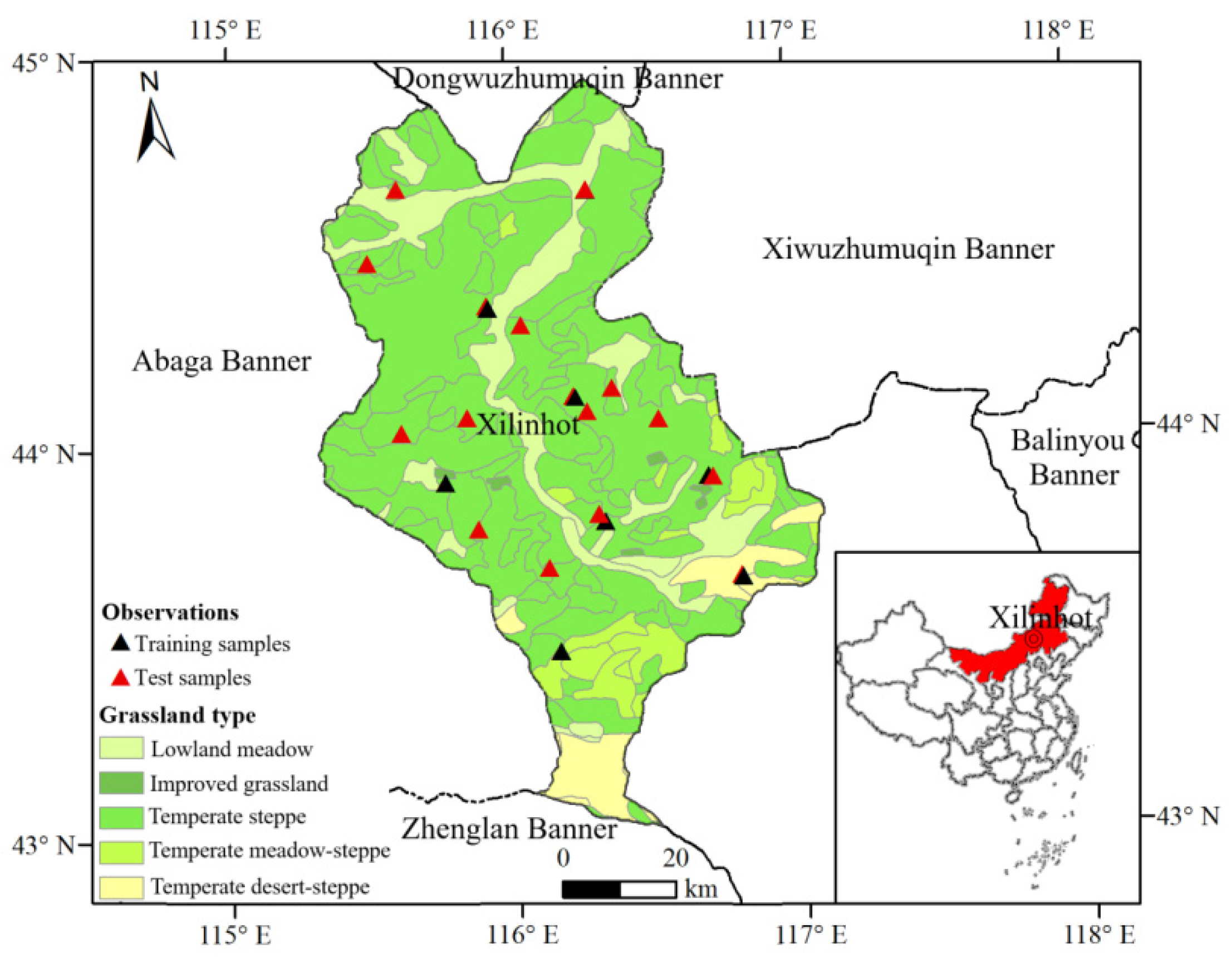
2.1. Study Area

The Xilinhot City of Inner Mongolia was chosen as the study area; it is located at 43°02′~44°52′N, 115°18′~117°06′E, covering a total area of approximately 14,785 km2 (Figure 1). The average altitude is 988.5 m, and the annual average precipitation is 295 mm, approximately. The annual average temperature is 2.6 °C. It is a semi-arid continental climate in the temperate zone, suitable for developing a grassland agro-ecosystem. A diverse grassland ecosystem has been formed here from superior geographic and climatic conditions. There are rich grassland types composed of lowland meadow, improved grassland, temperate steppe, temperate meadow steppe, and temperate desert steppe, with a wealth of dominant grass species in this region, including Cleistogenes squarrosa, L. chinensis, S. grandis, etc. In the past 20 years, the potential degraded area reached 162,200 km2 in Inner Mongolia, accounting for 20% of the total grassland area in Inner Mongolia, especially considering the moderately degraded grassland area of 47,600 km2 [28]. The central typical steppe region is one of the most degraded regions, including Xilinhot City [6]. Additionally, Xilinhot City is the seat of the Xilingol League region’s administrative center, forming the political, economic, cultural, and transportation center. Additionally, grassland resources are the city’s most important economic resource. Thus, it is important to ensure a grassland ecology balance in this area.

2.2. Data Collection and Preprocessing

This study collected data (Table 1) for grassland aboveground biomass simulation and used as direct or indirect inputs for grassland aboveground simulation and mapping, including observational, meteorology, satellite, and supplemental data.

2.2.1. Observational Data

Observational data refers to grassland aboveground biomass data observed in the field; 25 samples were separated into eight training samples and 17 test samples, distributed evenly throughout the study area (Figure 1). Observational data were obtained from the Institute of Agricultural Resources and Regional Planning, China Academy of Agriculture Sciences, as well as from the large-scale field campaign organized by the Grassland Monitoring and Supervision Center Ministry of Agriculture of China (GMSC) [29], primarily in August 2012, when green grassland was at its peak. Each sampling site had an area of 1 km2, with three sub-plots in each site measuring a distance greater than 250 m. The average weights of the three green parts and branches sub-plots were collected. Eight training samples were used to divide the study area into eight Thiessen zones, each of which contained only one point, with any position within it being closest to the same sample point, making full use of sparse observations to calibrate the model. Any location within a zone shares the exact and specific value of the model parameters.

2.2.2. Meteorology Data

Daily weather data were needed to drive the model in this study. Daily surface meteorological records of precipitation (Precip, mm), mean temperature (mTEM, °C), active photosynthetic radiation (PAR, MJ m−2), and crop evapotranspiration under standard conditions (ETC, mm day−1) were obtained from a 0.1° × 0.1° spatial resolution dataset named AgERA5. Available online: https://cds.climate.copernicus.eu/ (accessed on 23 May 2022). PAR was acquired from solar radiation flux with a conversion factor of 0.47 [30]. Daily ETC was equal to actual evapotranspiration (ET0), providing a crop coefficient of 1.15 [31], on the condition of obtaining ET0 from the Peman–Mandieth (PM) formula with several variables: solar radiation flux, 2 m maximum air temperature, 2 m mean air temperature, 2 m minimum air temperature, mean vapor pressure and 10 m mean wind speed.

2.2.3. Satellite Data

In this study, the LAI was considered the key state variable of data assimilation. The LAI time series were obtained from MODIS LAI products composited every four days at 500 m resolution on a sinusoidal grid named MCD15A3H. Available online: https://ladsweb.modaps.eosdis.nasa.gov/ (accessed on 23 May 2022). All the image time series of the MODIS LAI products were smoothed by fitting envelope and regression methods for two purposes: improving the daily temporal resolution to match the model and removing unreasonable or abnormal values.

2.2.4. Supplemental Data

The sand and clay content data for Xilinhot City were acquired from the Resource and Environment Science and Data Center, Chinese Academy of Sciences (CAS). Available online: https://www.resdc.cn/ (accessed on 23 May 2022). It can be converted to soil water-holding capacity (WHC, mm) [32]. Additionally, plant phenological information of grassland in Xilinhot City provided by the National Ecosystem Science Data Center, National Science & Technology Infrastructure of China, was utilized to modify the sum of temperatures profiling the period of growth in the simulation process [33].

2.3. Methods

Three main procedures were involved in this study for the realization of grassland aboveground biomass estimations (Figure 2): driving the ModVege model with parameter calibrations conducted through the MCMC method and assimilating the LAI from MCD15A3H products into the ModVege model to improve grassland aboveground biomass estimation. The ModVege model was mainly driven by four meteorological factors, including PAR, ET0, Precip, and mTEM, to simulate the dry weight of different grassland components. The likelihood functions of aboveground biomass (BM), leaf area index (LAI), and days when the accumulated temperature reached ST2, were constructed to generate multiple parameter combinations to drive the ModVege model. The MCMC algorithm was used to find the maximum likelihood values of the calibration parameters in different calibration zones, divided by Thiessen polygons according to the location of training points. The assimilation cost function was established according to 4DVar, and the state variable LAI (MOD15A3H products) was assimilated into the ModVege model pixel by pixel. The results of grassland aboveground biomass at a regional scale were then generated.

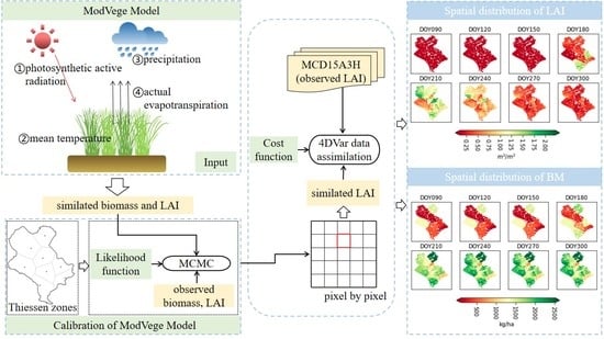
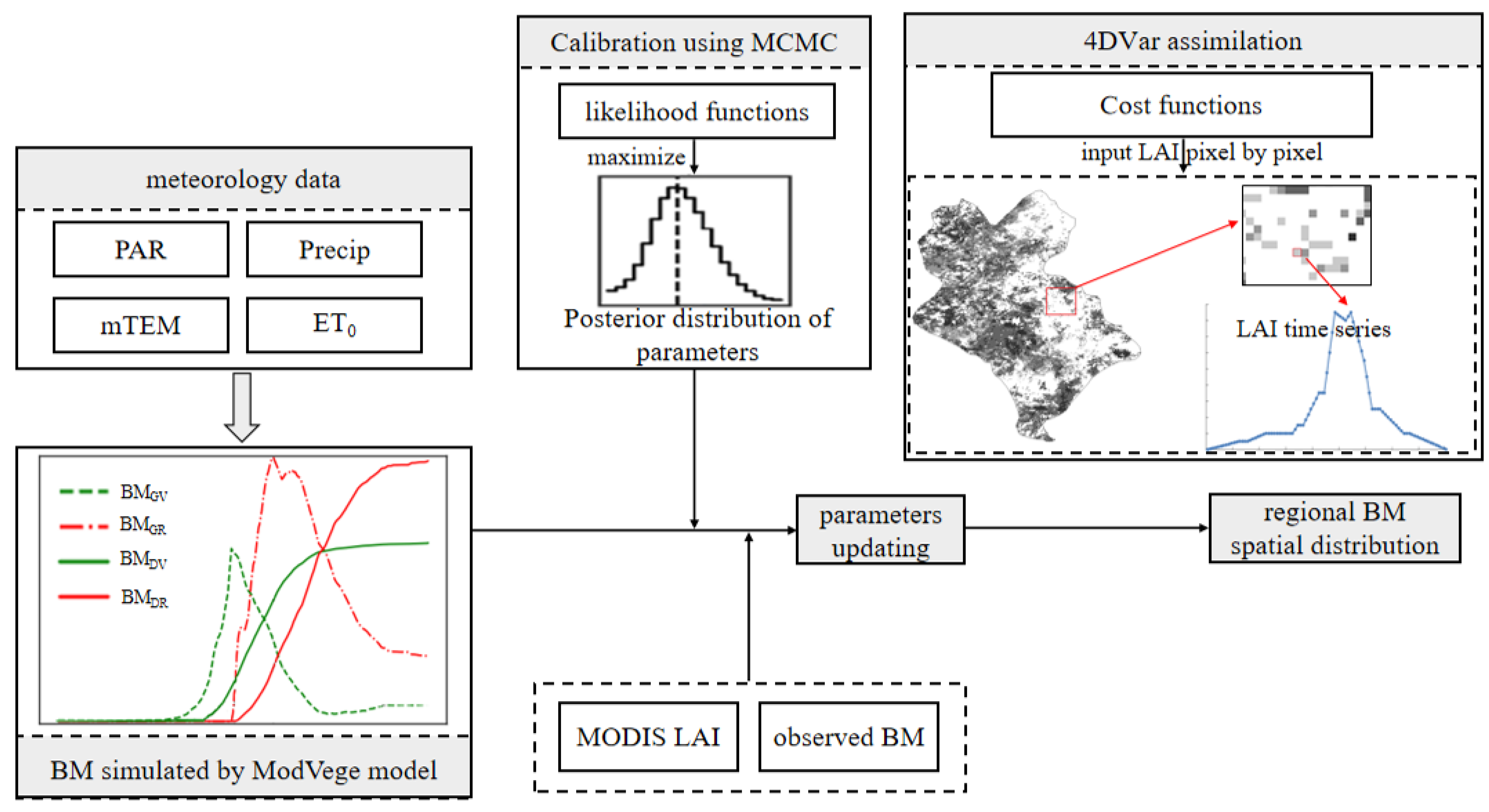
2.3.1. ModVege Model

The ModVege model is a mechanism model specializing in simulating the grassland growth process and its seasonal dynamic change, published by Jouven et al. [17,18]. The aboveground biomass is calculated daily between senescence and green compartments, according to the functions describing relationships between growth, senescence, and abscission with the environment. In this study, the ModVege model was developed in the programming language R, version 4.0.4, to simulate the aboveground biomass (BM) and leaf area index (LAI) [30]. The main parameters of the model and their values are shown in Table 2.
Grassland had low growth with flat and low values of LAI in the early (90 days) and latter (66 days) days of 2012. A rapid change period of LAI corresponding to all sampling points in the study area was selected as the time window for model simulation (Figure 3), occurring approximately from between the returning green stage to the seeding stage (DOY 90~DOY 310 of 2012).

2.3.2. Markov Chain Monte Carlo (MCMC)

Bayesian theory can infer the posterior distribution of parameters according to prior knowledge and the likelihood of model outputs. The relationship can be described as the following:
P ( θ | D ) = P ( D | θ ) P ( θ ) P ( D )
P ( θ | D ) and P ( D | θ ) represent the posterior distribution of parameters and likelihood function, respectively. P ( θ ) is the prior distribution of parameters, and P ( D ) stands for evidence, also known as the normalization constant. In the case of the ModVege model in this study, Equation (2) can be simplified as follows:
P ( θ | D , m ) = P ( D | θ ,   m ) P ( θ | m ) P ( D | m ) P ( D | θ , m ) P ( θ | m )
MCMC is a family of Bayesian analysis methods that provide an indirect way to sample from the posterior distribution. Firstly, a Markov chain (the first MC in MCMC) is identified, with its stationary distribution used as the posterior, thus sampling from this Markov chain. When it converges to its equilibrium distribution, the goal of sampling is essentially achieved. Unlike widely used point-estimate methods, such as the least square method and maximum likelihood estimation, the MCMC method can simultaneously provide unbiased estimates based on expectation and biased estimates from maximum likelihood and some mathematical statistics, such as quantile, covariance, and the spatial structure of parameters.
In this study, a differential evolution adaptive metropolis algorithm (DREAM) [34] was used to realize MCMC sampling through a Python package named SPOTPY [35]. Available online: https://github.com/thouska/spotpy.git (accessed on 23 May 2022).
(1) Parameters for calibration
LAI and BM are affected by five highly sensitive parameters, including ST1, ST2, LLS, BMGV0, and BMD0, which are selected as calibration parameters, with their prior distribution set to a uniform distribution. The prior distribution of calibration parameters is shown in Table 3.
(2) Likelihood function
In this study, a likelihood function for BM and LAI was constructed, also including days when the accumulated temperature reached ST2. The likelihood function is shown below.
l i k e 1 = 1 ( 2 π ) k | Σ | exp ( 1 2 ( LAI sim LAI obs ) T Σ 1 ( LAI sim LAI obs ) )
l i k e 2 = 1 2 π σ BM exp ( ( BM sim BM obs ) 2 2 σ BM 2 )
l i k e 3 = 1 2 π σ D O Y exp ( ( DOY sim DOY obs ) 2 2 σ D O Y 2 )
L = log ( l i k e 1 ) + log ( l i k e 2 ) + log ( l i k e 3 )
where L is the global likelihood function, l i k e 1 , l i k e 2 , and l i k e 3 are related to LAI, BM, and the day when the accumulated temperature reaches ST2, respectively. LAI sim and LAI obs are LAI simulated values and observed values when DOY is 228, BM sim and BM obs are BM simulated values and observed values, and DOY sim and DOY obs are the simulated day and actual day when the accumulated temperature reached ST2. K is the number of observations. ∑ is the covariance matrix of LAI, for which the standard deviation is assumed to be 30% of LAI. σ BM is the error of observation and equal to 10% of the observation in this study.   σ D O Y is the error of the day when the accumulated temperature reached ST2, which is set to 2d.

2.3.3. Four-Dimensional Variational (4Dvar) Data Assimilation

The cost function of 4Dvar comprehensively considers the uncertainty of the model parameters and the uncertainty of remote sensing observations. In this study, the cost function of 4Dvar is as follows:
J ( x ) = 1 2 [ x x b ] B 1 [ x x b ] + 1 2 ( L A I s i m L A I o b s ) T Σ 1 ( L A I s i m L A I o b s )
where x and x b both represent an array indicating ST2 and BMGV0, while x and x b are values after optimization and calibration, B is the covariance matrix of ST2 and BMGV0, and LAIsim and LAIobs are simulated and observed LAI time series. is the covariance matrix of MODIS LAI, simplified to a diagonal matrix here, and the standard deviation is defined as 30% of the corresponding observed values. Minimizing the cost function is based on a Python package named NLOPT. Available online: https://github.com/stevengj/nlopt (accessed on 23 May 2022).

2.3.4. Accuracy Evaluation Indexes

The mean absolute percentage error (MAPE) and root mean square error (RMSE) were used in this study to evaluate the simulation results of grassland aboveground biomass. The formulas are shown as follows:
MAPE = 100 % n i = 1 n | y ^ i y i y i |
where n is the number of measurements, y ^ i and y i are the simulated and measured values, respectively. The closer MAPE is to 0, the higher the simulation accuracy is.
RMSE = 1 n i = 1 n ( y ^ i y i ) 2
where n is the number of measurements, y ^ i and y i are the simulated and measured values, respectively. In this study, if the RMSE is a low value, it indicates a considerable simulation accuracy.

3. Results

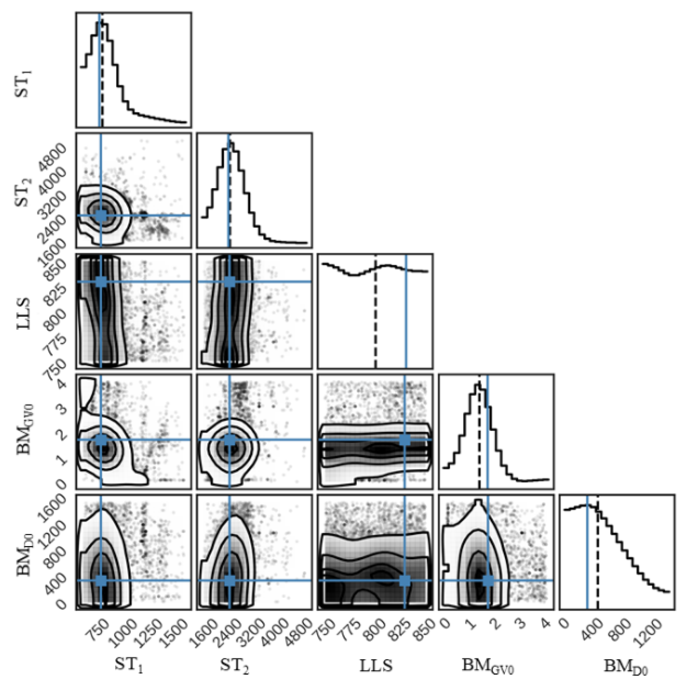
3.1. Calibration of ModVege Model

Based on the stationary distribution parameter samples being sampled by MCMC, the parameter uncertainty and posterior distribution can be inferred. The optimal parameter set of each zone is shown in Table 4. The posterior probability density of the parameters calibrated in Zone 8 (Figure 4) is taken as an example to quantitatively evaluate the ModVege model’s calibration effects. The five subgraphs on the diagonal of Figure 4 represent the posterior edge density of each parameter, and the two-dimensional projection between different parameters is the visualization of each parameter’s covariance. The solid lines in blue correspond to the maximum likelihood estimation of each parameter, and the black dashed lines demonstrate the 50% quantile of the posterior probability density distribution. Firstly, the posterior probability density distributions of ST1, ST2, BMGV0, and BMD0 are in the shape of a normal distribution, which is consistent with the hypothesis that the posterior distribution of MCMC is a normal distribution. At the same time, the posterior distribution of LLS has an abnormal distribution. The reason for this is that LLS is less sensitive than other parameters on the premise of a given observation and prior constraint as a concrete manifestation of large posterior uncertainty. Secondly, the maximum likelihood values are adjacent to the high-density area of each parameter distribution, which means that the calibration of the ModVege model can be taken as the optimal parameter values.
Figure 5 illustrates LAI and BM simulation uncertainties after calibration, with the shaded areas representing 95% confidence intervals of LAI and BM simulated by all the posterior calibration parameter assemblies and the solid lines indicating the point estimation results of LAI and BM obtained by only the maximum likelihood values of the parameters calibrated. As a whole, the uncertainty of the LAI gradually increases from the returning green stage (DOY is about 150) to the flowering stage (DOY is about 210), and the uncertainty reaches the maximum when the LAI curve peak is reached. With the decrease in LAI, its uncertainty also diminishes. The uncertainty of BM changes slightly in all periods and is relatively small in the period of rapid growth. The LAI simulated curve is consistent with the trend of MODIS LAI, increasing in the beginning and then decreasing and reaching a peak around DOY 200 in 2012.
The BM simulated curve remains stable and gradually increases from the turning green stage to the flowering stage and then decreases slightly after the flowering stage due to the biomass consumed by respiration being greater than that stored by photosynthesis. The simulated value of BM is close to the field observation value when DOY is 228, which confirms that the calibration of the ModVege model works.
The calibrated ModVege model was given 17 test samples; the accuracy is shown in Figure 6. Figure 6 shows that the BM observed value at the test points agrees with the simulated value, with R2 = 0.66. The overall simulation accuracy is great, with MAPE at 10% and an RMSE of 242 kg/ha. The simulation error may be caused by the difference between the test points and training points under soil, climate, and phenology conditions. It is hard for the model calibrated by the training points to perfectly simulate the test points. In addition, the operation of the model is mainly driven by weather factors, whose spatial resolution is relatively coarse, resulting in the mixed pixel effect that also affects the simulation accuracy.

3.2. The Spatial Variability Optimization of ST2 and BMGV0 Improve the Accuracy in Assimilation

Results of regional BM simulation illustrate an obvious spatial variability because, after assimilation at the pixel scale using the 4DVar algorithm, the spatial variability of ST2 and BMGV0 parameters increases significantly, as shown in Figure 7. The covariance of ST2 and BMGV0 can be calculated from posterior samples after calibration, valued between ± 25% of their maximum likelihood values. Compared with the results of parameter optimization before assimilation, ST2 and BMGV0 show obvious spatial heterogeneity after assimilation, which could effectively weaken the boundary effect after assimilation. In this study, ST2 indicates the accumulated temperature of grassland reaching the seed maturity stage. It can be concluded from Figure 7a that ST2 in the central regions of Xilinhot is higher than in other areas and reached the seed maturity stage later than grassland when compared to other regions with similar climatic conditions. In contrast, grassland in the northeast appears much earlier. BMGV0 represents the total aboveground biomass of leaves and leaf sheaths at the beginning of the simulation. As shown in Figure 7b, on DOY 90, BMGV0 in Northeastern regions is higher than in other areas, resulting from grassland having a relatively early turning greening stage.

3.3. Grassland Aboveground Biomass Estimation with the ModVege Model Using 4DVar Assimilation Xilinhot City

Figure 8 illustrates the spatial distribution of the LAI time series in of Inner Mongolia after assimilation in 2012. LAI shows a gradual increase from DOY 90 to DOY 270, a period of growth at the greatest rapidity. With the yellowing and withering of roots, stems, and leaves, LAI decreases, which is consistent with the growth cycle of grassland. When DOY is 180, 210, and 240, LAI presents prominent spatial differentiation characteristics that LAI: (1) features a spatial pattern that the high values concentrate in the southwest and east of Xilinhot City, while the western area is relatively low when DOY is 180; (2) is relatively high, but of the western areas is still lower than other areas, with the northwest area covered by high values, when DOY is 210; (3) shows a downward trend when DOY is 240. In other periods, grassland growth is slow, and LAI distributes relatively balanced.
Figure 9 illustrates the spatial distribution of the BM time series after assimilation for 2012. From DOY 90 to DOY 150, the aboveground biomass of grassland shows obvious spatial variability, and the biomass is higher in the western and northeastern areas but lower in other areas. BM changes dramatically from DOY 180 and gradually becomes stable after DOY 210. Overall, the northeast grassland aboveground biomass is higher than in other areas, especially central and southeastern. The reason for this is that the central areas are close to urbanized land and frequent human activities, meaning climate conditions for grassland growth are susceptible to disturbance, and the southeastern areas covered desert steppe are generally occupied by drought-resistant and low-yielding grassland.
The simulation results of LAI and BM show an apparent boundary effect in spatial pattern, especially when grassland grows slowly, resulting from that LAI values as state variables are stable and low for a long time during this period, which has a little constraint on assimilation trajectory. The main factor affecting the simulation results is the meteorological input of the ModVege model, which is highly uniform in space for its coarse resolution, making it easy to cause insignificant differences in BM and LAI between adjacent pixels but apparent variation in the regions. During the period of rapid growth, the blocking phenomenon and boundary effect gradually weaken for the state variables (remotely sensed LAI) at play in the assimilation, giving rise to the spatial variability enlargement of simulated LAI and BM.
As shown in Figure 10, all testing points are distributed near the 1:1 trend line, indicating that the simulated value of BM after assimilation is in great agreement with the observed, with an R2 value of 0.62. The accuracy improved after the assimilation, with MAPE at 10% and RMSE rising to 214 kg/ha.

4. Discussion

In this study, a mechanism approach was compromised and applied to estimate aboveground biomass in large grassland areas using the assimilation method. The essence of this was to use strict mathematical theory to optimize the parameters to conform to the vegetation growth mechanism. The implemented approach provides a feasible means to estimate the grassland aboveground biomass. With this approach, BM and the LAI can be qualified efficiently. This approach could simulate LAI and vegetation BM by assimilating leaf area index into the model. This study proves the applicability of the remote sensing data assimilation method to simulate and predict grassland aboveground biomass at a large scale based on the machine model available. Previous studies of grassland aboveground biomass estimation at a large scale were usually conducted via empirical models instead of mechanism models, in which the parameters are hard to estimate and the accuracy tended to be questionable [36].
In addition, compared with other research, the accuracy of the empirical model was improved by approximately 20% [37]. After assimilation, this study improved the RMSE from 242 kg/ha to 214 kg/ha. Several studies with mechanism models have also been conducted to quantify BM, but only at the point scale without being generalizable to other regions [38,39] with an RMSE greater than 500 kg/ha. This study realized the regional application of the grassland growth process model and the data assimilation method on a regional scale, which had not been realized in previous studies. The assimilation method was adopted for regional extension. Still, the crop model was used instead of the grassland model [25], and the accuracy from He et al. [23] is less than that of this study, with an RMSE of 617.94 kg/ha without considering the point scale [24]. is less than that of this study with RMSE = 617.94 kg/ha. Or even make it to the point scale [24]. In general, very few studies have been carried out using mechanical models in the region. This study has realized the shortcomings of the above studies and has potential for regional application.
The most valuable advantage of the mechanism model is that it can quantify the causal relationship between environment and growth, which provides a concept to study and deal with grassland governance within the context of global climate change in the future. It can help decision makers and landowners gain a timely understanding of grassland distribution, growth status and environmental dynamics compared with the same period from previous years, and facilitating the adoption of management measures, or be utilized as important information for agricultural insurance. The method implemented in this study mainly relies on meteorological data [40]. Therefore, it can be applied to other regions with well-calibrated processed-based models. It can also provide early warnings for grassland management by combining future climate data with real-time predictions. In addition, it can be applied to a larger area under suitable computational conditions and sufficient sample data [41,42]. Moreover, the relationship between the growth trend and growth factors revealed by the model can also provide directions for governing, preventing, and improving grassland ecology.
In this study, grassland species were not strictly distinguished, and the assimilation accuracy was limited due to the lack of multi-temporal growth information on grassland. Grassland management measures (such as harvesting, etc.), phenological information, and soil characteristics of different grassland types should also be focused on to overcome the bottleneck of various grassland-type simulations in the future. Moreover, to improve the accuracy of assimilation, the spatial resolution of remotely sensed images needs to be finer, and the corresponding computing pressure also needs to be solved synchronously. At the same time, the deep learning method constrained by the mechanism model provides a promising approach to improving accuracy [43,44]. The errors in this study were mainly caused by the input data and initial values of the parameters in the ModVege model. (1) In terms of input data quality, the observed BM values are obtained from the wet weights to corresponding dry weights with 15% water content to match the simulated BM from ModVege, according to the grassland type [45]. However, due to the uncertainty of de-watering, there will be errors in the accuracy of verification results. The spatial resolution of MODIS LAI data is rough [46]. At the same time, the process models such as the ModVege model are relatively precise and have high accuracy at the point scale if the inputs are fairly accurate. Pixels maxed with different features exist in MODIS LAI, and outliers affected by cloud and rain cannot meet the process model’s precision requirements, leading to uncertainty of the simulation results. (2) Only one period of observed BM time series was captured. To ensure that the trajectory of calibration converges well in the whole simulation time series, MODIS LAI, the same as that in the assimilation process, was added into the cost function, resulting in minimal space for improving the accuracy after assimilation. (3) In the case of uncertainty from the parameter values of the ModVege model, there is a lack of in-field reference of the initial values for some parameters that are less sensitive to the results, such as BMR0 endowed with default values and WHC obtained by the conversion of soil texture [47]. Although the simulation result has a slight impact, errors are still accumulating in the simulation process.

5. Conclusions

In this study, a data assimilation approach was implemented to simulate grassland aboveground biomass using the ModVege model using the four-dimensional variational algorithm (4DVar), with the city of Xilinhot, Inner Mongolia, used as the study area. MCMC was used to calibrate the ModVege model effectively, and five parameters highly sensitive to the results were selected to be calibrated. The uncertainty of the BM estimates, formed by random and systematic effects, are quantitatively described, further revealing the interpretability of mechanism models used for grassland growth simulation and intuitively showing the range of possible simulation results on the entire time series. The BM simulated by the calibrated model was close to that of the field observation values. The uncertainty was small in the rapid growth period of grassland, demonstrating that the assimilation strategy with the ModVege model used in this study is feasible for estimating the aboveground biomass of grassland. To better use the assimilation method for the retrieval of large-scale grassland growth and the pursuit of accurate biomass estimates for further improvement, methods for quantifying the uncertainty of the observations should be introduced, allowing for quality-conscious input data to be generated.

Author Contributions

Conceptualization, Y.Z. (Yuxin Zhang), J.H. and H.H.; Methodology, Y.Z. (Yuxin Zhang), J.H. and H.H.; Writing-original draft, Y.Z. (Yuxin Zhang); Writing—review and editing, J.H., H.H. and X.L.; Data support, Y.J.; Supervision, H.G., Q.F. and Y.Z. (Yuanyuan Zhao). All authors have read and agreed to the published version of the manuscript.

Funding

This research is supported by the National Key R&D Program of China (project No.2018YFE0122700) and the National Natural Science Foundation of China (project No. 41971383).

Acknowledgments

We thank the journal’s editors and anonymous reviewers for their kind comments and valuable suggestions to improve the quality of this paper.

Conflicts of Interest

The authors declare no conflict of interest.

References

  1. Da Silveira Pontes, L.; Maire, V.; Schellberg, J.; Louault, F. Grass strategies and grassland community responses to environmental drivers: A review. Agron. Sustain. Dev. 2015, 35, 1297–1318. [Google Scholar] [CrossRef]
  2. Xie, G.D.; Zhang, Y.L.; Lu, C.X.; Zheng, D.; Cheng, S.K. Study on valuation of rangeland ecosystem services of China. J. Nat. Resour. 2001, 16, 47–53. [Google Scholar] [CrossRef]
  3. Altesor, A.; Oesterheld, M.; Leoni, E.; Lezama, F.; Rodríguez, C. Effect of grazing on community structure and productivity of a Uruguayan grassland. Plant Ecol. 2005, 179, 83–91. [Google Scholar] [CrossRef]
  4. Zhao, B.Y.; Liu, Z.Y.; Lu, H.; Wang, Z.X.; Sun, L.S.; Wan, X.P.; Guo, X.; Zhao, Y.T.; Wang, J.J.; Shi, Z.C. Damage and Control of Poisonous Weeds in Western Grassland of China. Agric. Sci. China 2010, 9, 1512–1521. [Google Scholar] [CrossRef]
  5. Zhang, Y.; Zhang, C.B.; Wang, Z.Q.; Yang, Y.; Zhang, Y.Z.; Li, J.L.; An, R. Quantitative assessment of relative roles of climate change and human activities on grassland net primary productivity in the Three-River Source Region, China. Acta Prataculturae Sin. 2017, 26, 1–14. [Google Scholar] [CrossRef]
  6. Ma, M.; Zhang, S.W.; Wei, B.C. Temporal and Spatial Pattern of Grassland Degradationand Its Determinants for Recent 30 Years in Xilingol. Chin. J. Grassl. 2017, 39, 86–93. [Google Scholar] [CrossRef]
  7. Shen, G.R.; Wang, R.C. Review of the application of vegetation remote sensing. J. Zhejiang Univ. (Agric. Life Sci.) 2001, 27, 682–690. [Google Scholar] [CrossRef]
  8. Nakano, T.; Bavuudorj, G.; Urianhai, N.G.; Shinoda, M. Monitoring aboveground biomass in semiarid grasslands using MODIS images. J. Agric. Meteorol. 2013, 69, 33–39. [Google Scholar] [CrossRef] [Green Version]
  9. Liu, Y.; Nie, L.; Yang, Y. Estimation of the total production of the herbage in the Tianshan Mountain Area using remote sensing technology with NDVI similarity zoning. Pratacultural Sci. 2018, 35, 1754–1764. [Google Scholar] [CrossRef]
  10. Zhou, X.; Sheng, J.D.; Zhang, W.T.; Wu, H.Q.; Wang, X.J. Aboveground Biomass Inversion of Grassland in Ili Area Using MODIS Data. Acta Agrectir. Sin. 2015, 23, 27–33. [Google Scholar] [CrossRef]
  11. Reiche, M.; Funk, R.; Zhang, Z.D.; Hoffmann, C.; Reiche, J.; Wehrhan, M.; Li, Y.; Sommer, M. Application of satellite remote sensing for mapping wind erosion risk and dust emission-deposition in Inner Mongolia grassland, China. Grassl. Sci. 2012, 58, 8–19. [Google Scholar] [CrossRef]
  12. Chen, P.F.; Wang, J.L.; Liao, X.Y.; Yin, F.; Chen, B.R.; Liu, R. Using Data of HJ-1A/B Satellite for Hulunbeier Grassland Aboveground Biomass Estimation. J. Nat. Resour. 2010, 25, 1122–1131. [Google Scholar] [CrossRef]
  13. Wang, Y.J.; Wang, J.L.; Wei, H.S.; Altansukh, O.; Davaadorj, D.; Sonomdagva, C. Study on estimation method of Mongolia grassland production based on sparse samples. J. Geo-Inf. Sci. 2020, 22, 1814–1822. [Google Scholar] [CrossRef]
  14. Xun, Q.L.; Dong, Y.Q.; An, S.Z.; Yan, K. Monitoring of grassland herbage accumulation by remote sensing using MOD09GA data in Xinjiang. Acta Prataculturae Sin. 2018, 27, 10–26. [Google Scholar] [CrossRef]
  15. Johnson, I.R.; Thornley, J.H.M. Vegetative crop growth model incorporating leaf area expansion and senescence, and applied to grass. Plant Cell Environ. 1983, 6, 721–729. [Google Scholar] [CrossRef]
  16. Brereton, A.J.; Danielov, S.A.; Scott, D. Agrometeorology of Grass and Grasslands for Middle Latitudes; World Meteorological Organisation: Geneva, Switzerland, 1996. [Google Scholar]
  17. Jouven, M.; Carrere, P.; Baumont, R. Model predicting dynamics of biomass, structure and digestibility of herbage in managed permanent pastures. 1. Model description. Grass Forage Sci. 2006, 61, 112–124. [Google Scholar] [CrossRef]
  18. Jouven, M.; Carrere, P.; Baumont, R. Model predicting dynamics of biomass, structure and digestibility of herbage in managed permanent pastures. 2. Model evaluation. Grass Forage Sci. 2006, 61, 125–133. [Google Scholar] [CrossRef]
  19. Hurtado-Uria, C.; Hennessy, D.; Shalloo, L.; Schulte, R.P.O.; Delaby, L.; O’Connor, D. Evaluation of three grass growth models to predict grass growth in Ireland. J. Agric. Sci. 2012, 151, 91–104. [Google Scholar] [CrossRef] [Green Version]
  20. Katata, G.; Grote, R.; Mauder, M.; Zeeman, M.J.; Ota, M. Wintertime grassland dynamics may influence belowground biomass under climate change: A model analysis. Biogeosciences 2020, 17, 1071–1085. [Google Scholar] [CrossRef] [Green Version]
  21. Quaife, T.; Lewis, P.; Dekauwe, M.; Williams, M.; Law, B.E.; Disney, M.; Bowyer, P. Assimilating canopy reflectance data into an ecosystem model with an Ensemble Kalman Filter. Remote Sens. Environ. 2008, 112, 1347–1364. [Google Scholar] [CrossRef]
  22. Migliavacca, M.; Meroni, M.; Busetto, L.; Colombo, R.; Zenone, T.; Matteucci, G.; Manca, G.; Seufert, G. Modeling Gross Primary Production of Agro-Forestry Ecosystems by Assimilation of Satellite-Derived Information in a Process-Based Model. Sensors 2009, 9, 922–942. [Google Scholar] [CrossRef] [PubMed] [Green Version]
  23. He, B.B.; Li, X.; Quan, X.W.; Qiu, S. Estimating the Aboveground Dry Biomass of Grass by Assimilation of Retrieved LAI into a Crop Growth Model. IEEE J. Sel. Top. Appl. Earth Obs. Remote Sens. 2015, 8, 550–561. [Google Scholar] [CrossRef]
  24. Huang, X.; Zhao, G.; Zorn, C.; Tao, F.L.; Ni, S.Q.; Zhang, W.Y.; Tu, T.; Hoglind, M. Grass modelling in data-limited areas by incorporating MODIS data products. Field Crop Res. 2021, 271, 108250. [Google Scholar] [CrossRef]
  25. Zhang, X.T.; He, B.B.; Quan, X. Assimilation of 30 m resolution LAI into crop growth model for improving LAI estimation in plateau grassland. In Proceedings of the International Geoscience and Remote Sensing Symposium (IGRASS), Beijing, China, 10–15 July 2016; pp. 1296–1299. [Google Scholar] [CrossRef]
  26. Huang, J.X.; Sedano, F.; Huang, Y.B.; Ma, H.Y.; Li, X.L.; Liang, S.L.; Tian, L.Y.; Zhang, X.D.; Fan, J.L.; Wu, W.B. Assimilating a synthetic Kalman filter leaf area index series into the WOFOST model to improve regional winter wheat yield estimation. Agric. For. Meteorol. 2016, 216, 188–202. [Google Scholar] [CrossRef]
  27. Huang, J.X.; Tian, L.Y.; Liang, S.L.; Ma, H.Y.; Becker-Reshef, I.; Huang, Y.B.; Su, W.; Zhang, X.D.; Zhu, D.H.; Wu, W.B. Improving winter wheat yield estimation by assimilation of the leaf area index from Landsat TM and MODIS data into the WOFOST model. Agric. For. Meteorol. 2015, 204, 106–121. [Google Scholar] [CrossRef] [Green Version]
  28. Wu, N.T.; Liu, G.X.; Yang, Y.; Song, X.Y.; Bai, H.H. Dynamic monitoring of net primary productivity and its response to climate factors in native grassland in Inner Mongolia using a light-use efficiency model. Acta Prataculturae Sin. 2020, 29, 1. [Google Scholar]
  29. Jin, Y.X.; Yang, X.C.; Qiu, J.J.; Li, J.Y.; Gao, T.; Wu, Q.; Zhao, F.; Ma, H.L.; Yu, H.D.; Xu, B. Remote Sensing-Based Biomass Estimation and Its Spatio-Temporal Variations in Temperate Grassland, Northern China. Remote Sens. 2014, 6, 1496–1513. [Google Scholar] [CrossRef] [Green Version]
  30. Calanca, P.; Deleglise, C.; Martin, R.; Carrere, P.; Mosimann, E. Testing the ability of a simple grassland model to simulate the seasonal effects of drought on herbage growth. Field Crops Res. 2016, 187, 12–35. [Google Scholar] [CrossRef]
  31. Allen, R.G.; Pereira, L.S.; Raes, D.; Smith, M. Crop Evapotranspiration-Guidelines for Computing Crop Water Requirement-FAO Irrigation and Drainage Paper 56, 1st ed.; FAO: Rome, Italy, 1998; pp. 17–20. [Google Scholar]
  32. Saxton, K.E.; Rawls, W.J.; Romberger, J.S.; Papendick, R.I. Estimating generalized soil-water characteristics from texture. Soil Sci. Soc. Am. J. 1986, 50, 1031–1036. [Google Scholar] [CrossRef]
  33. Chinese Ecosystem Research Network. Plant phenological observation dataset of the Chinese Ecosystem Research Network (2003–2015) [DB/OL]. Sci. Data Bank 2017, 10. [Google Scholar] [CrossRef]
  34. Vrugt, J.A. Markov chain Monte Carlo simulation using the DREAM software package: Theory, concepts, and MATLAB implementation. Environ. Model. Softw. Environ. Data News 2016, 75, 273–316. [Google Scholar] [CrossRef] [Green Version]
  35. Houska, T.; Kraft, P.; Chamorro-Chavez, A.; Breuer, L. SPOTting Model Parameters Using a Ready-Made Python Package. PLoS ONE 2015, 10, e145180. [Google Scholar] [CrossRef] [PubMed]
  36. Li, H.L.; Zhao, J. Principles and methods of grassland yield estimation by using remote sensing technology. Pratacultural Sci. 2009, 3, 34–38. [Google Scholar] [CrossRef]
  37. Zhao, F.; Xu, B.; Yang, X.C.; Jin, Y.X.; Li, J.Y.; Xia, L.; Chen, S.; Ma, H.L. Remote Sensing Estimates of Grassland Aboveground Biomass Based on MODIS Net Primary Productivity (NPP): A Case Study in the Xilingol Grassland of Northern China. Remote Sens. 2014, 6, 5368–5386. [Google Scholar] [CrossRef] [Green Version]
  38. Ruellea, E.; Hennessya, D.; Delabyb, L. Development of the Moorepark St Gilles grass growth model (MoSt GG model): A pre-dictive model for grass growth for pasture based systems. Eur. J. Agron. 2018, 99, 89–91. [Google Scholar] [CrossRef]
  39. Korhonen, P.; Palosuo, T.; Persson, T.; Höglind, M.; Jégo, G.; Oijen, M.V.; Gustavsson, A.M.; Bélanger, G.; Virkajärvia, P. Modelling grass yields in northern climates—A comparison of three growth models for timothy. Field Crops Res. 2018, 224, 37–47. [Google Scholar] [CrossRef]
  40. McDonnell, J.; Brophya, C.; Ruelle, E.; Shalloo, L.; Lambkin, K.; Hennessy, D. Weather forecasts to enhance an Irish grass growth model. Eur. J. Agron. 2019, 105, 168–175. [Google Scholar] [CrossRef]
  41. Huang, H.; Huang, J.X.; Li, X.C.; Zhuo, W.; Wu, Y.T.; Niu, Q.D.; Su, W.; Yuan, W.P. A dataset of winter wheat aboveground biomass in China during 2007–2015 based on data assimilation. Sci. Data 2022, 9, 200. [Google Scholar] [CrossRef]
  42. Huang, J.X.; Gómez-Dans, J.L.; Huang, H.; Ma, H.Y.; Wu, Q.L.; Lewis, P.E.; Liang, S.L.; Chen, Z.X.; Xue, J.H.; Wu, Y.T.; et al. Assimilation of remote sensing into crop growth models: Current status and perspectives. Agric. For. Meteorol. 2019, 276–277, 107609. [Google Scholar] [CrossRef]
  43. Xie, Y.; Huang, J.X. Integration of a Crop Growth Model and Deep Learning Methods to Improve Satellite-Based Yield Estimation of Winter Wheat in Henan Province, China. Remote Sens. 2021, 13, 4372. [Google Scholar] [CrossRef]
  44. Wang, X.L.; Huang, J.X.; Feng, Q.L.; Yin, D.Q. Winter wheat yield prediction at county level and uncertainty analysis in main wheat-producing regions of China with deep learning approaches. Remote Sens. 2020, 12, 1744. [Google Scholar] [CrossRef]
  45. Fang, J.Y.; Liu, G.H.; Xu, S.L. Carbon Pools in Terrestrial Ecosystems in China. In Emissions and Their Relevant Processes of Greenhouse Gases in China, 1st ed.; Wang, G.C., Wen, Y.P., Eds.; China Environment Science Press: Beijing, China, 1996; pp. 109–128. [Google Scholar]
  46. Schaffrash, D.; Barthold, F.K.; Bernhofer, C. Spatiotemporal variability of grassland vegetation cover in a catchment in Inner Mongolia, China, derived from MODIS data products. Plant Soil 2011, 340, 181–198. [Google Scholar] [CrossRef]
  47. Cheng, Y.; Cai, Z.C.; Zhang, J.B.; Lang, M.; Mary, B.; Chang, S.X. Soil moisture effects on gross nitrification differ between adjacent grassland and forested soils in central Alberta, Canada. Plant Soil 2012, 352, 289–301. [Google Scholar] [CrossRef]
Figure 1. Grassland type and observation distribution in the study area.
Remotesensing 14 03194 g001
Figure 2. Flowchart of the study methods. Noted abbreviations are: PAR (photosynthetic active radiation), Precip (precipitation), mTEM (mean temperature), ET0 (actual evapotranspiration), LAI (leaf area index), MCMC (Markov chain Monte Carlo), BM (biomass), and 4DVar (four-dimensional variational)).
Remotesensing 14 03194 g002
Figure 3. MODIS LAI distribution at sampling sites from DOY 1 to DOY 366 of 2012. Solid green dots from light to dark indicate the number of sampling points with the same LAI value.
Remotesensing 14 03194 g003
Figure 4. Posterior distribution of parameters.
Remotesensing 14 03194 g004
Figure 5. Uncertainties of LAI and BM simulation after calibration.
Remotesensing 14 03194 g005
Figure 6. Accuracy evaluation of simulated BM and observed BM after calibration.
Remotesensing 14 03194 g006
Figure 7. ST2 and BMGV0 spatial distribution after assimilation.
Remotesensing 14 03194 g007
Figure 8. Spatial distribution pattern of LAI in Xilinhot City of Inner Mongolia after assimilation.
Remotesensing 14 03194 g008
Figure 9. Spatial distribution of BM in Xilinhotcity of Inner Mongolia after assimilation.
Remotesensing 14 03194 g009
Figure 10. Accuracy evaluation of BM simulation after assimilation.
Remotesensing 14 03194 g010
Table 1. Data overview for grassland aboveground biomass simulation.
CategoryDatasetResolutionYear
Observational datagrassland aboveground biomass observations\2012
Meteorology dataAgERA5 datasetdaily2012
Satellite dataMCD15A3H (LAI)500 m/4 days2012
Supplemental dataLUCC dataset1000 m2013
Soil texture data1000 m\
Plant phenological observation dataset\\
Table 2. Main parameters of the ModVege model.
NotationUnitDescriptionValue
SLAm2/gSpecific leaf area0.0256
minSEA-The minimum value of the seasonal factor0.67
LAM%Percentage of laminae0.68
RUEmaxg/MJMaximum radiation use efficiency3
maxSEA-The maximum value of the seasonal factor1.33
T0°CdMinimum temperature for photosynthesis4
T1°CdMinimum temperature for maximum photosynthetic rate10
T2°CdMaximum temperature for maximum photosynthetic rate20
KGV°CdSenescence rate, green vegetative tissues0.002
KGR°CdSenescence rate, green reproductive tissues0.001
KlDV°CdAbscission rate, dead vegetative tissues0.001
KlDR°CdAbscission rate, dead reproductive tissues0.0005
SGVd−1Rate of biomass loss with respiration, green vegetative tissues0.4
SGRd−1Rate of biomass loss with respiration, green reproductive tissues0.2
NI-Nutrition index0.88
Table 3. Prior distribution of calibration parameters.
ParameterDescriptionRange
LLS (°Cd)Leaf lifespan[600, 900]
ST1 (°Cd)Temperature sum defining the start of reproductive growth[600, 1600]
ST2 (°Cd)Temperature sum defining the end of reproductive growth[1600, 5000]
BMGV0Initial biomass, green vegetative tissues[0.01, 4.0]
BMD0Initial biomass, dead vegetative and reproductive tissues[0.01, 1500]
Table 4. The optimal parameter values of different zones after calibration.
ZonesParameters
ST1 (°Cd)ST2 (°Cd)LLS (°Cd)BMGV0BMD0
11062.002500.00793.500.19460519.50
21350.002628.00796.500.075561327.00
3619.002168.00752.003.97300479.20
4862.002356.00770.500.5260063.53
5696.502328.00821.503.87500312.80
61393.002672.00752.501.07100139.50
71370.002674.00751.001.374001471.00
81160.002544.00771.500.5310044.50
Publisher’s Note: MDPI stays neutral with regard to jurisdictional claims in published maps and institutional affiliations.

