Article

Assimilating C-Band Radar Data for High-Resolution Simulations of Precipitation: Case Studies over Western Sumatra

1
Climate and Weather Disasters Collaborative Innovation Center, School of Applied Meteorology, Nanjing University of Information Science & Technology, Nanjing 210044, China
2
Department of Atmospheric Sciences, University of Utah, Salt Lake City, UT 84112, USA
3
The Agency for Meteorology, Climatology, and Geophysics of the Republic of Indonesia, Jakarta 10720, Indonesia
4
State Key Laboratory of Atmospheric Boundary Layer Physics and Atmospheric Chemistry, Institute of Atmospheric Physics, Chinese Academy of Sciences, Beijing 100029, China
*
Author to whom correspondence should be addressed.
Remote Sens. 2022, 14(1), 42; https://doi.org/10.3390/rs14010042
Submission received: 14 October 2021 / Revised: 19 December 2021 / Accepted: 20 December 2021 / Published: 23 December 2021

Abstract

:
Accurate high-resolution precipitation forecasts are critical yet challenging for weather prediction under complex topography or severe synoptic forcing. Data fusion and assimilation aimed at improving model forecasts, as one possible approach, has gained increasing attention in past decades. This study investigates the influence of the observations from a C-band Doppler radar over the west coast of Sumatra on high-resolution numerical simulations of precipitation around its vicinity under the Madden–Julian oscillation (MJO) in January and February 2018. Cases during various MJO phases were selected for simulations with an advanced research version of the weather research and forecasting (WRF) model at a cloud-permitting scale (~3 km). A 3-dimensional variational (3DVAR) data assimilation method and a hybrid three-dimensional ensemble–variational data assimilation (3DEnVAR) method, based on the NCEP Gridpoint Statistical Interpolation (GSI) assimilation system, were used to assimilate the radar reflectivity and the radial velocity data. The WRF-simulated precipitation was validated with the Integrated Multi-satellitE Retrievals for GPM (IMERG) precipitation data, and the fractions skill score (FSS) was calculated in order to evaluate the radar data impacts objectively. The results show improvements in the simulated precipitation with hourly radar data assimilation 6 h prior to the simulations. The modifications with assimilation were validated through the observation departure and moist convection. It was found that forecast improvements are relatively significant when precipitation is more related to local-scale convection but rather small when the background westerly wind is strong under the MJO active phase. The additional simulation experiments, under a 1- or 2-day assimilation cycle, indicate better improvements in the precipitation simulation with 3DEnVAR radar assimilation than those with the 3DVAR method.

Graphical Abstract

1. Introduction

The Maritime Continent (MC), which includes islands of various sizes, forms, and terrain types [1], lies along the equator between the Indian Ocean and the Pacific Ocean, with a zonal width of more than 5000 km [2]. Many studies have shown the MC’s essential role in the global weather-climate continuum [3,4,5,6]. For instance, the Madden–Julian oscillation (MJO) [7,8], a significant fluctuation in tropical weather, can interact with the MC on weekly to monthly timescales. MJO’s large-scale tropical disturbance usually propagates eastward at a speed of approximately 5 m s−1, with a typical zonal extent of roughly 12,000–20,000 km and a period of 30–90 days [9]. Therefore, an MJO passing the MC or being blocked by the MC could have noticeable impacts on MC local weather, including the local rainfall. Significant modulations of the spatial and temporal distribution of precipitation have been found in many studies [10,11,12,13,14]. The different MJO phases indicate various locations of convection-favoring disturbance. Therefore, understanding MC weather characteristics during these phases has been an essential research topic. Accurate simulations of MC convection and precipitation by numerical models are challenging, due to complex terrain and surface features, coarse model resolutions, and deficiencies in model physics [15,16,17,18]. Furthermore, with sparse in situ observations over western Sumatra, accurate numerical weather prediction must rely largely on appropriate analysis and initial conditions.
High-resolution precipitation forecasts are an essential part of accurate weather and climate prediction under complex topography or severe synoptic forcing. Data assimilation is a method used to achieve an optimal combination of short-range forecasts and observations. It has received increasing attention during the past decade as a useful method to help to improve high-resolution precipitation forecasts. Besides conventional data assimilation, which is widely used in model forecasts in many regions, radar data assimilation has been developed simultaneously in recent years. Based on the investigation of a well-documented supercell storm that occurred near Del City, Oklahoma, Gao and Stensrud [19] explored the impact of assimilating radar reflectivity and radial velocity data with a 3DVAR system. Lat et al. [20] introduced an improved approach to derive a pseudo-water vapor mass mixing ratio and in-cloud potential temperature in southern China. Radhakrishnan and Chandrasekar [21] blended a radar-based nowcast with a numerical weather prediction (NWP) model over the Dallas–Fort Worth (DFW) urban radar network, aimed at improving predictive ability with a 6-h lead time. However, there has been little progress over the MC region, owing to the lack of radar data.
Based on the support of the Meteorology, Climatology, and Geophysical Agency (BMKG), Indonesia, radar data are available for part of Sumatra. The International Years of Maritime Continent (YMC) program provides an opportunity to widely study the impacts of radar data assimilation on local weather forecasting through international collaboration. This study aimed to conduct a series of experiments in order to investigate the impacts of the assimilating data obtained from a single radar around Padang, a station in western Sumatra, Indonesia, on the simulations of local-scale convection and precipitation. Considering the influence of the MJO on weather conditions, we intend to understand the large-scale conditions under which radar data can be useful for local weather forecasting. Therefore, this paper attempts to examine the radar data assimilation under different phases of an MJO event from November 2017 to February 2018 [22]. The convective disturbance passed over Padang from the middle to the end of January.
The rest of the paper is organized as follows: Section 2 introduces the numerical simulation experiments, the data assimilation configuration, and the precipitation verification method; Section 3 presents all of the results, including the convection description, precipitation verification, assimilation impacts, and the synoptic background analysis; Section 4 gives a discussion with existing literature; Section 5 summarizes all of the concluding remarks.

2. Cases and Model Set-Up
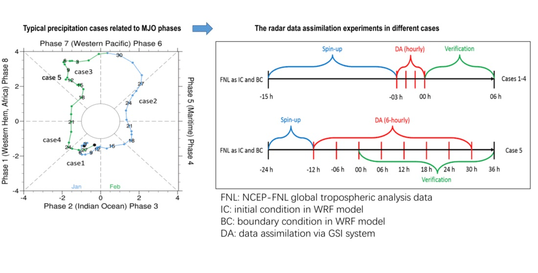
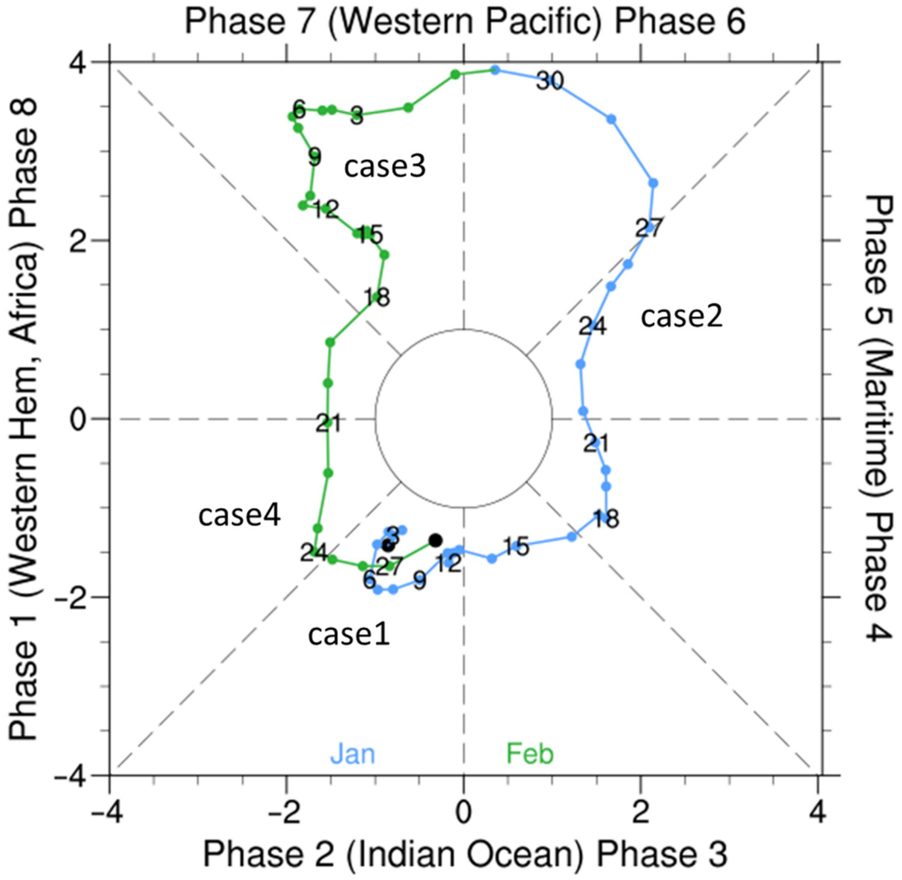
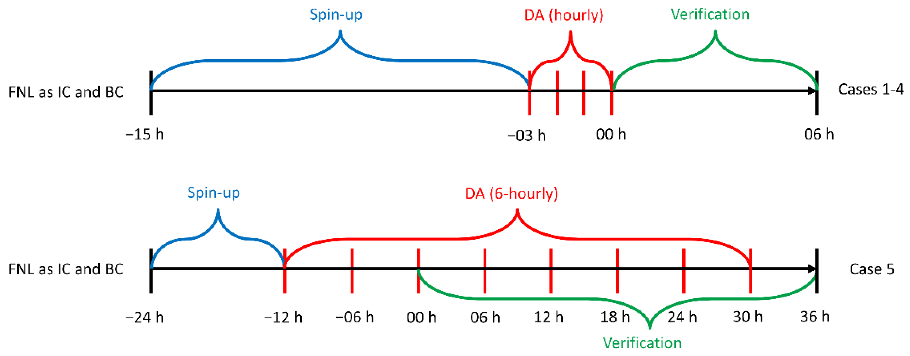
2.1. Case Durations

An RMM phase diagram describing the MJO event based on the method proposed by Wheeler and Hendon [23] is presented in Figure 1, with data provided by the Australian Bureau of Meteorology.
The four representative convective cases were selected based on the availability of radar data, each with a time span of 6 h. The durations and corresponding MJO phases for these cases are as follows: 1500 UTC 7 January–2100 UTC 7 January in phase 2 (Case 1), 0000 UTC 24 January–0600 UTC 24 January in phase 5 (Case 2), 2100 UTC 11 February–0300 UTC 12 February in phase 7 (Case 3), and 1800 UTC 22 February–0000 UTC 23 February in phase 1 (Case 4), as marked in Figure 1. According to the partitioning of the MJO life cycle mentioned by Wei et al. [24], Case 1 is in the MC preconditioning stage, Case 2 is in the MC active stage, and Cases 3 and 4 are in the MC suppressed stage. The MJO amplitude during each case is always larger than one, revealing non-negligible modulations of the MJO on the large-scale synoptic background. Most of this paper focuses on simulations within 6 h, since previous literature has shown that the impacts of radar data assimilation are most apparent within short-term (usually up to 6 h) forecasts [25,26,27,28,29].
A summary of the case durations is presented in Table 1, including the starting and ending times of simulations after data assimilation. Note that an additional case, Case 5, from 1200 UTC 11 February to 0000 UTC 13 February was added as an extension of Case 3. While hourly radar data assimilation was conducted before the 6-h simulations in Cases 1–4, the purpose of Case 5 was to verify the impacts of 6-hourly data assimilation before and during the 36-h simulations, where apparent short-term impacts from radar data assimilation could be refreshed every 6 h throughout the modeling period.

2.2. WRF Model Configuration

An advanced research version of the weather research and forecasting (WRF) model version 4.0 [30] was employed in order to conduct the numerical simulations with radar data assimilation. The NCEP-FNL 0.25° × 0.25° global tropospheric analysis data [31] were utilized as initial conditions and 3-hourly lateral boundaries during the simulations. A single domain was configured in the WRF model, with a horizontal resolution of 3 km and a grid span of 1080 × 720, covering all of Sumatra and the surrounding ocean. The topography within the domain is shown in Figure 2. A total of 40 vertical layers were configured, with the model top at 50 hPa.
For the physical scheme configuration, the tropical suite set that was predefined in WRF, and that has performed well in tropical areas, was applied, as follows: the WRF single-moment 6-class graupel scheme [32] with ice, snow, and graupel processes suitable for the microphysics option in high-resolution simulations, the RRTMG scheme [33] for the longwave/shortwave radiation option, the Yonsei University scheme [34] for the boundary-layer option, the MM5 scheme [35] for the surface-layer option, and the Unified Noah land-surface model [36] for the land-surface option. The default tropical suite configured the parameterized convection utilizing the new Tiedtke scheme [37], while among all of the simulations in this study, the explicit convection, rather than the parameterized convection, was configured under the cloud-permitting horizontal resolution of 3 km.

2.3. Radar Data and GSI Assimilation System

The reflectivity and radial velocity data from a ground-based C-band Doppler radar over Padang, Indonesia, had a spatial coverage shown by the red circle in Figure 2 (where the black cross indicates the radar’s location). The resolution was 1 km horizontally and 0.5 km vertically, within a horizontal measurement range of 250 km and a vertical measurement range of 12.5 km. The steep topography to the east of the radar blocked the lowest elevation angles, and quality control was conducted to remove the topography-affected data.
The community Gridpoint Statistical Interpolation (GSI) system [38] was applied for the radar data assimilation in this study. The following two assimilation methods were selected: the 3-dimensional variational (3DVAR) [39] method for all cases, and the hybrid EnKF–3DVAR (3DEnVAR) method [40], combining the 3DVAR and ensemble Kalman filter (EnKF) method, for Case 5 only.
The cost function in the 3DVAR assimilation method is as follows:
J ( x ) = 1 2 ( x x b ) T B 1 ( x x b ) + 1 2 ( y H [ x ] ) T R 1 ( y H [ x ] )
where x is the analysis field, xb is the background field, B is the background-error covariance matrix, H is the observation operator, y is the observation field, and R is the observation-error covariance matrix. The minimization of the cost function generates the result for data assimilation. The background-error covariance plays an important role in determining how the information from the observations is spread to nearby grid points and levels [41]. In GSI, the static regional background-error covariance for 3DVAR is obtained through the interpolation of NCEP’s NAM model forecasts onto background grids.
In the 3DEnVAR method, the forecast error covariance (equivalent to B in Equation (1)) is obtained from a linear combination of the 3DVAR covariance B 3 D V a r [42], as follows:
P f ( h y b r i d ) = ( 1 a ) P f + a B 3 D V a r
where a is a tunable parameter to determine the ratio of the impacts from 3DVAR and EnKF (0.5 as equal weighting in this study), and P f is the estimate of the EnKF forecast error covariance from the K forecasts x k f ( t i ) after completing the ensemble of analyses at time t i 1 , as follows:
P f 1 K 1 k = 1 K ( x k f x ¯ f ) ( x k f x ¯ f ) T
where the overbar represents the ensemble average. In this study, the NCEP GFS global EnKF 80 ensemble members [43] helped to achieve the flow-dependent background-error covariance, weighting the background forecasts and observations more appropriately [44].
The GSI system automatically interpolated the radar reflectivity horizontally and vertically to match the grids in the WRF simulations. After radar reflectivity interpolation and assimilation, the cloud analysis option was turned on in GSI with the input of the cloud water, cloud ice, rain, snow, and graupel as first-guess. The procedure within GSI introduced by Hu et al. [45] combines the strengths of early-developed semi-empirical cloud analysis packages. Ingestion of background fields and observations is followed by stable/convective cloud analysis.
For the radial velocity assimilation, the GSI system applied a super-ob process developed by Purser et al. [46], in which the radial velocity data available within a given time window, for example, no more than 0.5 h sooner or later than the assimilation timestamp, were separated and included within different boxes with a coarser spatial resolution, and then averaged within each super-ob box. This process helps to reduce the redundant information and the data density and is aimed at better fitting data assimilation systems and forecasting models [47]. The parameter configurations during the super-ob process are also summarized in Table 1. The minimum number of observations in a super-ob box, namely the observation density threshold, was set at 30 according to comparisons of model behaviors against different density thresholds in this study. Any observations with a lower density in each box were not used for assimilation.

2.4. Experiment Design and Verification

Figure 3 describes the spin-up periods, data assimilation cycles, and case simulations, where the FNL data always provided the initial and boundary conditions (IC and BC). In the control (CTL) experiment in Cases 1–4, instead of conducting a freely running simulation, we assimilated the NCEP ADP global upper-air and surface weather observations [48] (namely, the conventional data) in a 3-h assimilation window after a 12-h spin-up. For the 3DVAR experiments (3DV), available radar data within this assimilation window were additionally integrated. Taking Case 1 (1500 UTC 7 January~2100 UTC 7 January) as an example, in the CTL experiment, the 12-h spin-up lasted from 0000 UTC 7 to 1200 UTC 7, and then available conventional data were assimilated from 1200 UTC to 1500 UTC, followed by a 6-h simulation to be verified against IMERG precipitation data. In the 3DV experiment, the hourly radar data assimilation was added from 1200 UTC to 1500 UTC. Here, 00 h is defined as the beginning of the 6-h simulation, so the spin-up was from −15 h to −03 h, while the conventional data and radar data were assimilated hourly from −03 h to 00 h. The half time window is one of the adjustable parameters for data ingestion and assimilation in the GSI assimilation system. For the experiments in Cases 1–4, the default value of 0.5 h was applied, which means that all of the conventional data or radar data available with a temporal difference of no more than 0.5 h from the assimilation timestamp were used.
In Case 5, spin-up lasted from −24 h to −12 h, while the 6-hourly data assimilation in CTL, 3DV, and the hybrid 3DEnVAR (HYB) followed at −12 h, −06 h, and 00 h, as revealed in Figure 3. In contrast to Cases 1–4, where assimilation was conducted only before the verification period, assimilation in Case 5 also occurred throughout the 36-h simulation, with an interval of 6 h, so the apparent short-term impacts from assimilation covered the whole simulation period. For the assimilation experiments in Case 5, the half time window was modified to 1 h through sensitivity tests that indicated a slightly better performance compared with those configured with the default 0.5 h.
The precipitation verification was emphasized in this study. The 0.1° × 0.1° half-hourly Integrated Multi-satellitE Retrievals for GPM (IMERG) [49] V06B final run precipitation products [50] produced by NASA were employed to validate the model-produced precipitation, which was horizontally interpolated onto IMERG grids using inverse distance weighting. To objectively assess the quantitative precipitation forecast (QPF) skill among the different cases and experiments, a scale-selective verification introduced by Roberts and Lean [51] was applied in order to calculate the fractions skill score (FSS) under various thresholds and neighborhood lengths, as follows:
FSS ( n , p ) = 1 i = 1 N x j = 1 N y [ O ( n , p ) i , j M ( n , p ) i , j ] 2 i = 1 N x j = 1 N y [ O ( n , p ) i , j 2 + M ( n , p ) i , j 2 ]
where N x and N y are the total number of columns and rows in the whole field to be verified. Given neighborhood length n and threshold p , the variable O is the fraction of observation grids with values exceeding threshold p (recognized as a “hit”) within a total of n × n observation grids centered at column i and row j , while M is the fractional variable for the simulation grids. The calculated FSS represents the averaged behaviors against the different thresholds, at different locations, and within different ranges, and it showed a higher tolerance to location shifts commonly noticeable in high-resolution simulations, which can suffer a greater punishment through traditional point-to-point skill scores and can reflect high-resolution performance more objectively. In this study, neighborhood length n ranged up to 100 km, approximately 10 times the IMERG grid resolution of 0.1°, indicating that a location shift of ±5 grids was recognized as a hit prediction.
The integrated surface database (ISD) [52] produced by the National Centers for Environmental Information (NCEI) was additionally included for in situ precipitation measurements. Two Indonesian sites, Tabing (0.9°S, 100.4°E) and Japura Airport (0.4°S, 102.3°E), were available within the study area, as marked in Figure 2. During the 5 cases in this paper, there were very few ISD samples at the two sites, making a direct validation of the WRF simulations nearly impossible. Instead, validation of the IMERG data was carried out by horizontal interpolation onto those sites during all of January and February 2018, covering all cases. A high correlation with the ISD data was expected to confirm the good quality of the IMERG data and to make the conclusions from the model assessments more convincing, as judged by the statistics of bias (BIAS), root mean square error (RMSE), and Pearson correlation coefficient (PCC), calculated as follows:
BIAS = i = 1 n ( y i x i ) n
RMSE = i = 1 n ( y i x i ) 2 n
PCC = i = 1 n ( y i y ¯ ) ( x i x ¯ ) i = 1 n ( y i y ¯ ) 2 i = 1 n ( x i x ¯ ) 2
where x and y are the ISD and IMERG precipitation samples (mm h−1) with a total number n and corresponding averages x ¯ and y ¯ .

3. Results

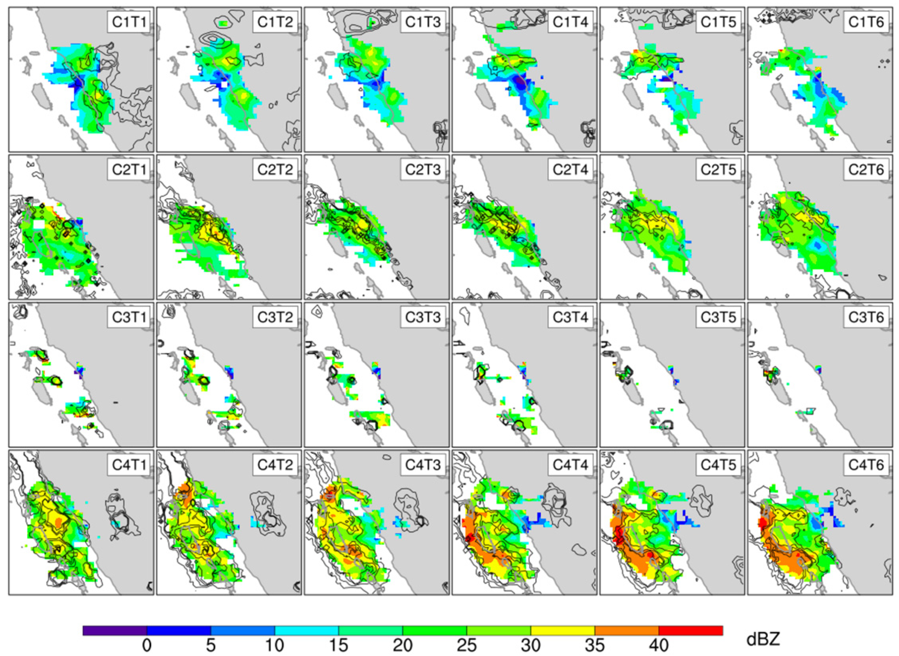
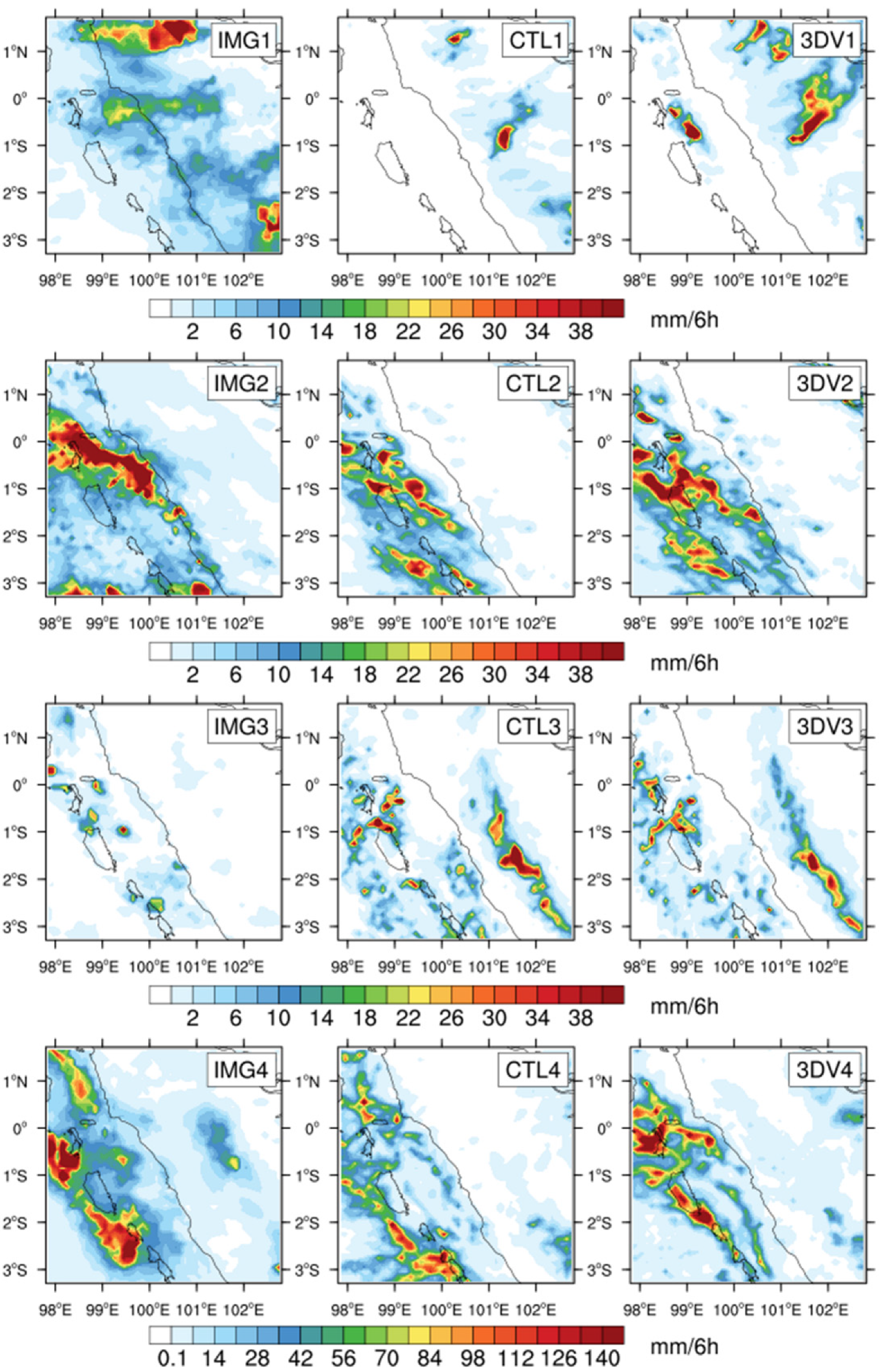
3.1. Convection Description

Figure 4 shows the spatial distribution of Padang radar reflectivity and IMERG precipitation rate during 01 h–06 h in Cases 1–4. Convective bands were available around the western coast in Case 1, and MJO phase 2 (P2) occurred during the MC preconditioning stage. At 01 h, precipitation formed to the east of the Barisan mountains along the western coast, and seaward migration took place from 03 h to 05 h both near Padang and to the north. The patterns in Case 2 under MJO P5 were the opposite, as follows: the convective bands accumulated near the coast and land until 03 h, but the migration afterwards was slightly eastward and landside precipitation formed at 06 h. The landward migration during an MC active phase was also revealed by Yokoi et al. [53]. In Case 3, the convection and precipitation under MJO P7 were much weaker than in Cases 1 and 2. The convective cells were generated near the western coast and spread seaward, likely caused by factors such as cold land surges or gravity waves. The exact mechanism was not investigated in this study, but it remains an interesting topic for future study. Case 4 occurred during MJO P1 (the MC suppressed stage) and is the case with the heaviest convection and precipitation as well as obscured migration, which might arise from a strong synoptic background, such as strengthened low-level westerly wind and convergence.

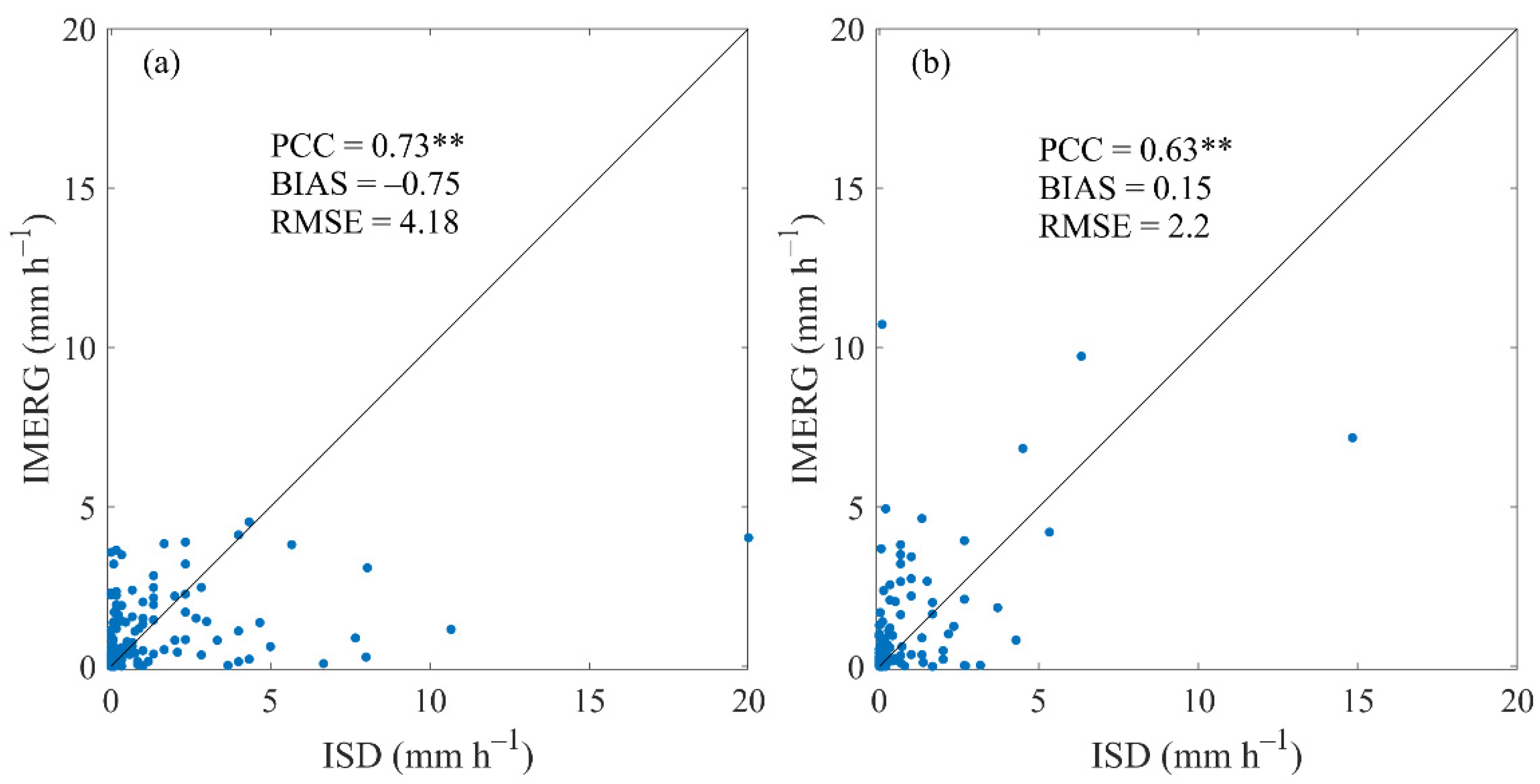
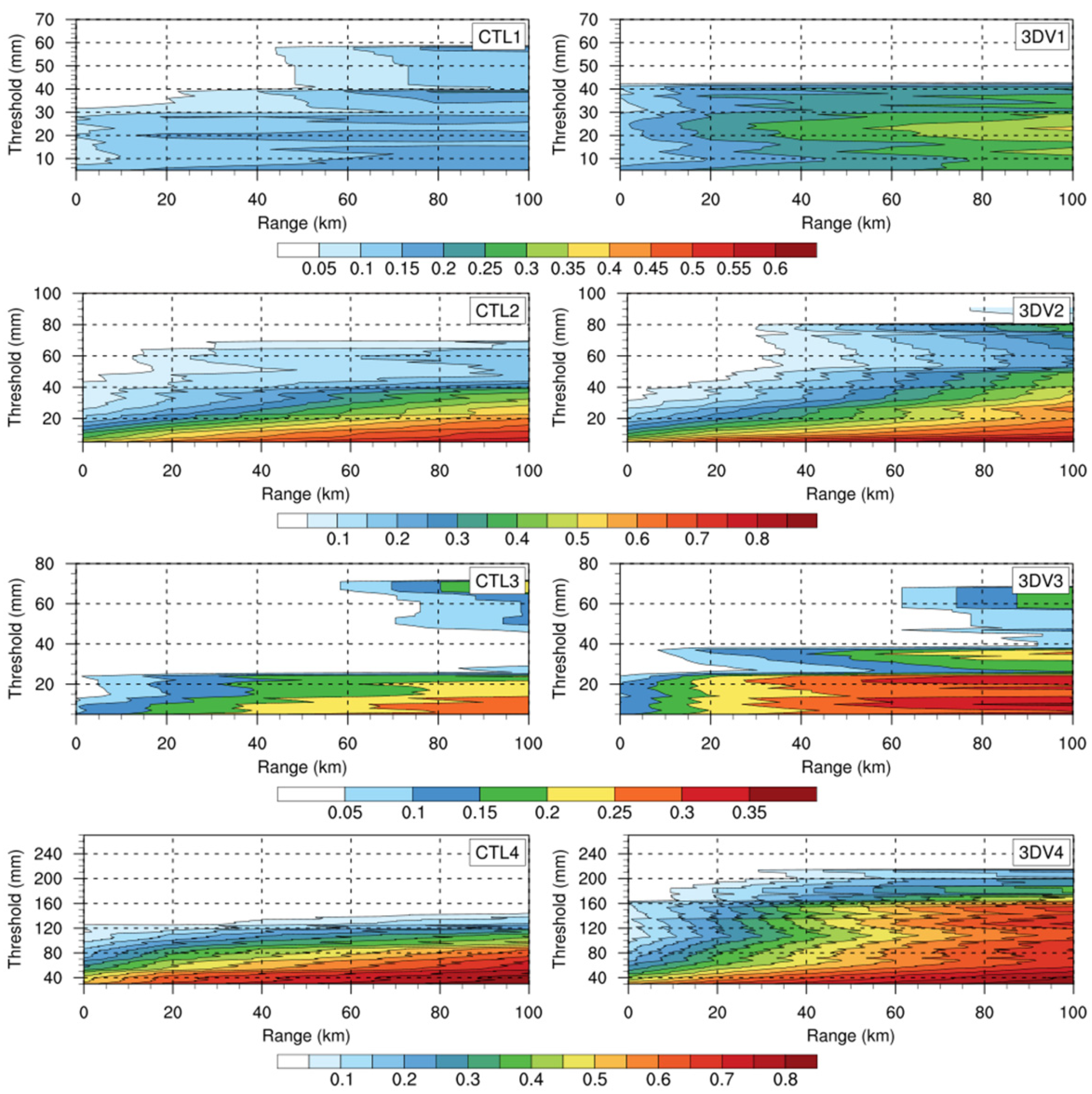
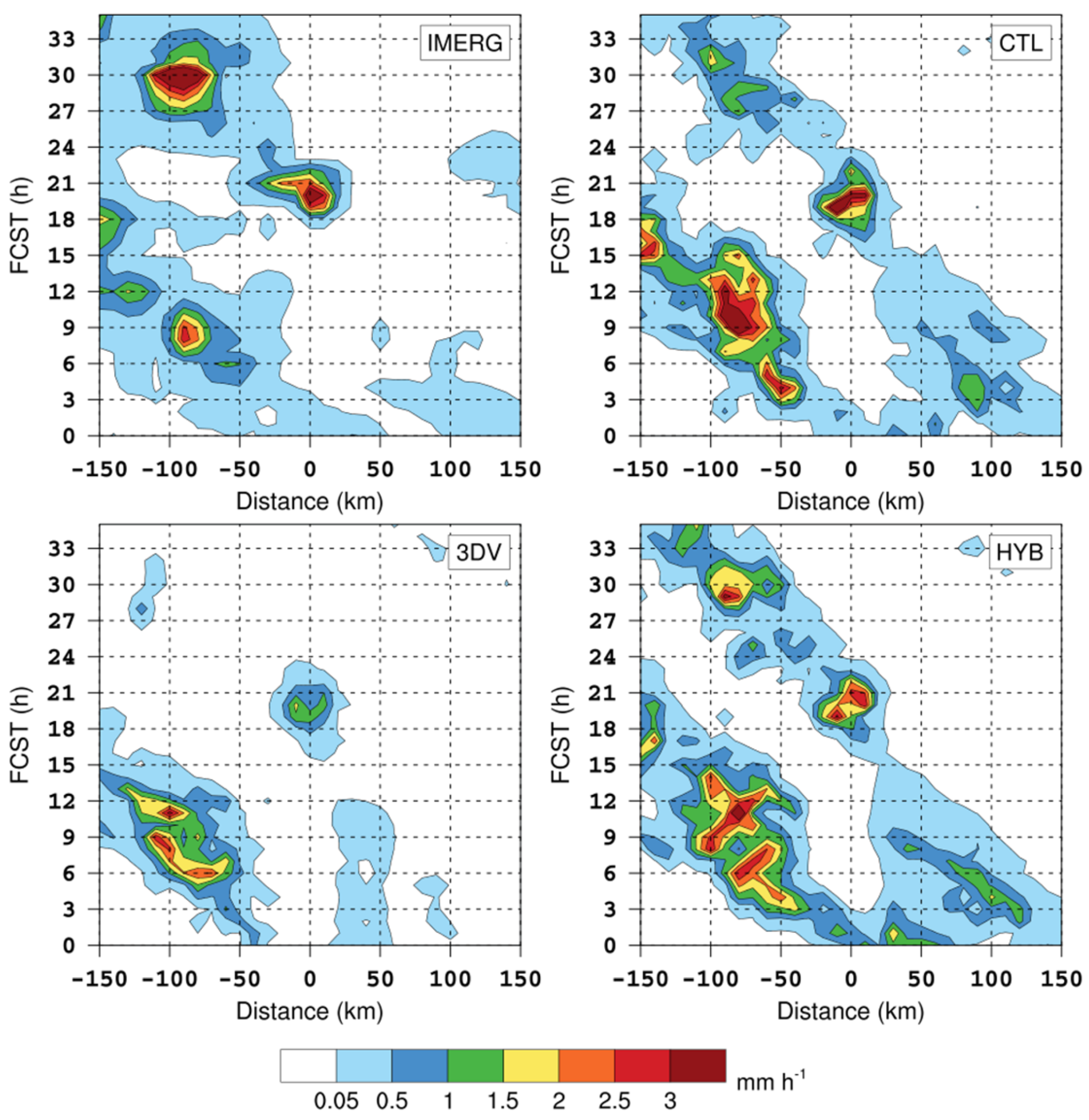
3.2. Precipitation Verification

Figure 5 compares the hourly precipitation rate at Tabing and Japura Airport from the ISD measurements and from IMERG interpolations during January and February 2018. The PCC was estimated at 0.73 and 0.63, respectively, both significant at the 0.01 level according to the Student′s t-test, reflecting a moderate to high correlation between the ISD and the IMERG data. The BIAS was −0.75 mm h−1 and 0.15 mm h−1, while the RMSE was 4.18 mm h−1 and 2.20 mm h−1. Despite the few ISD samples available for model validation during each case included in this study, the comparison with IMERG samples suggests that the model validation against the IMERG data should generally be valuable.
Figure 6 shows the accumulated precipitation from IMERG and WRF in Cases 1–4. The two precipitation zones lie across the west coast in Case 1, one near Padang and the other to the north, consistent with the migration in Figure 4. The CTL underestimation in the north was largely reduced in 3DV. The mountain precipitation near Padang in IMERG was not well reproduced even after assimilation; instead, it occurred farther offshore and caused coastal overestimation in 3DV. Despite that, the total precipitation quantity around Padang was still closer to IMERG.
In Case 2 the CTL simulation performed well in spatial patterns and quantities, probably because the precipitation was modulated mostly by large-scale synoptic backgrounds in order to ensure the simulation was not ruined by poor response to coastal topography. The 3DV impacts on the spatial distribution were neutral, partly due to the difficulty of further improving the model behaviors that were fine in CTL. There was an issue in Case 2, in that WRF significantly underestimated coastal precipitation, while neither conducting radar data assimilation nor increasing the model′s vertical levels from 40 to 60, noticeably improving the behaviors. The two-way nesting was configured with an outer domain as coarse as 9 km in the surroundings, with a finer (3 km) inner domain covering the area of radar data. That configuration was considered a possible reason for the poor model behaviors. Further investigation should be done in the future with this case, as the initial conditions (data assimilation) were not the major influencing factor. Rather, physical processes may play a more important role here.
The CTL experiment exhibited a slight overestimation in the seaside and landside areas in Case 3, which was somewhat reduced in the 3DV experiment. Relative to Cases 1 and 2, improvements in the precipitation simulation with assimilation in Case 3 were weaker, probably arising from weaker convection with a lower rain rate and fewer samples in Case 3 (Figure 4). In contrast, during the heavy precipitation of Case 4 with large areas of convection, the radar captured abundant precipitation samples (Figure 3), which was conducive to good simulations of the two precipitation centers around Siberut in the 3DV experiment.
Figure 7 displays the FSS scores calculated from the CTL and 3DV experiments in Cases 1–4 with the scale-selective verification method introduced in Section 2.4. The range was calculated by multiplying the grid length (approximately 10 km for 0.1°) by the number of the neighborhood grid points, namely n in Equation (4). The maximum threshold p was determined as the maximum accumulated precipitation within the whole region during each case, and the minimum was set at 5 mm in Cases 1–3 and 30 mm in the heavy precipitation case (Case 4). The CTL scores were higher in Cases 2 and 4, the two cases without visible seaward migration of precipitation. The 3DV improvements were noticeable in Cases 1, 3, and 4 but were minor in Case 2, consistent with the spatial comparison (Figure 4). As described in Section 3.1, in Case 2 the precipitation migration was slightly landward in the MC convective active stage of MJO, affected by the stronger onshore background wind, which significantly enhanced vapor advection as the dominant factor of precipitation. However, no radar data assimilation was conducted farther offshore to modify this advection from the northern Indian Ocean, which is assumed to be a possible reason for the minor DA improvements in Case 2. Further discussion about synoptic impact is given in Section 3.4.

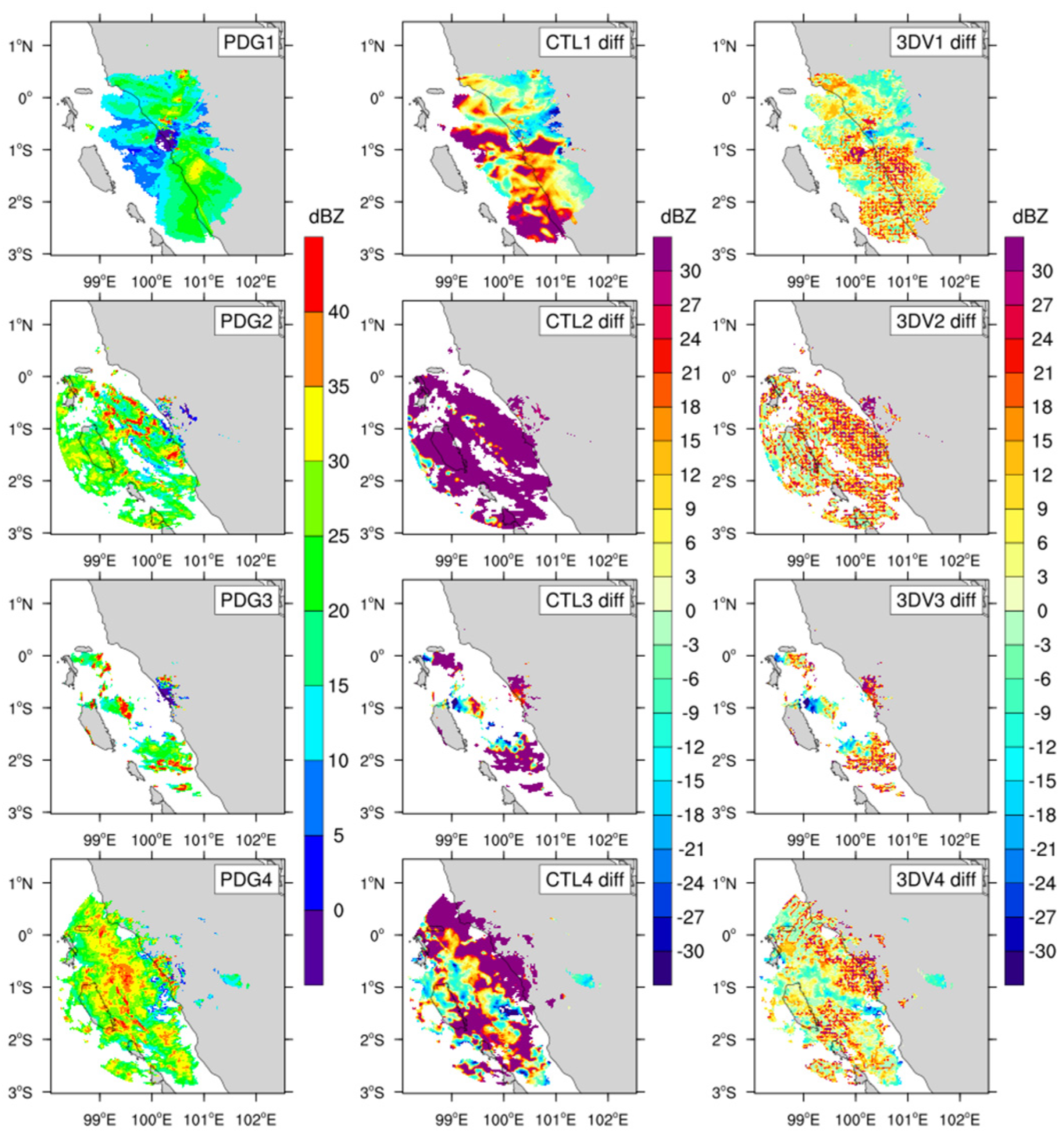
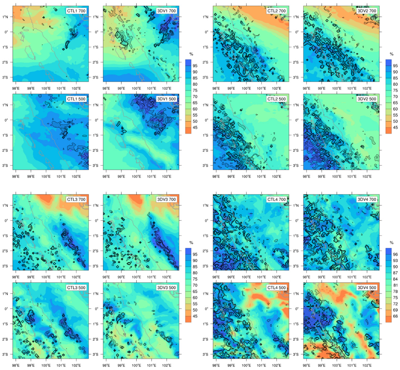
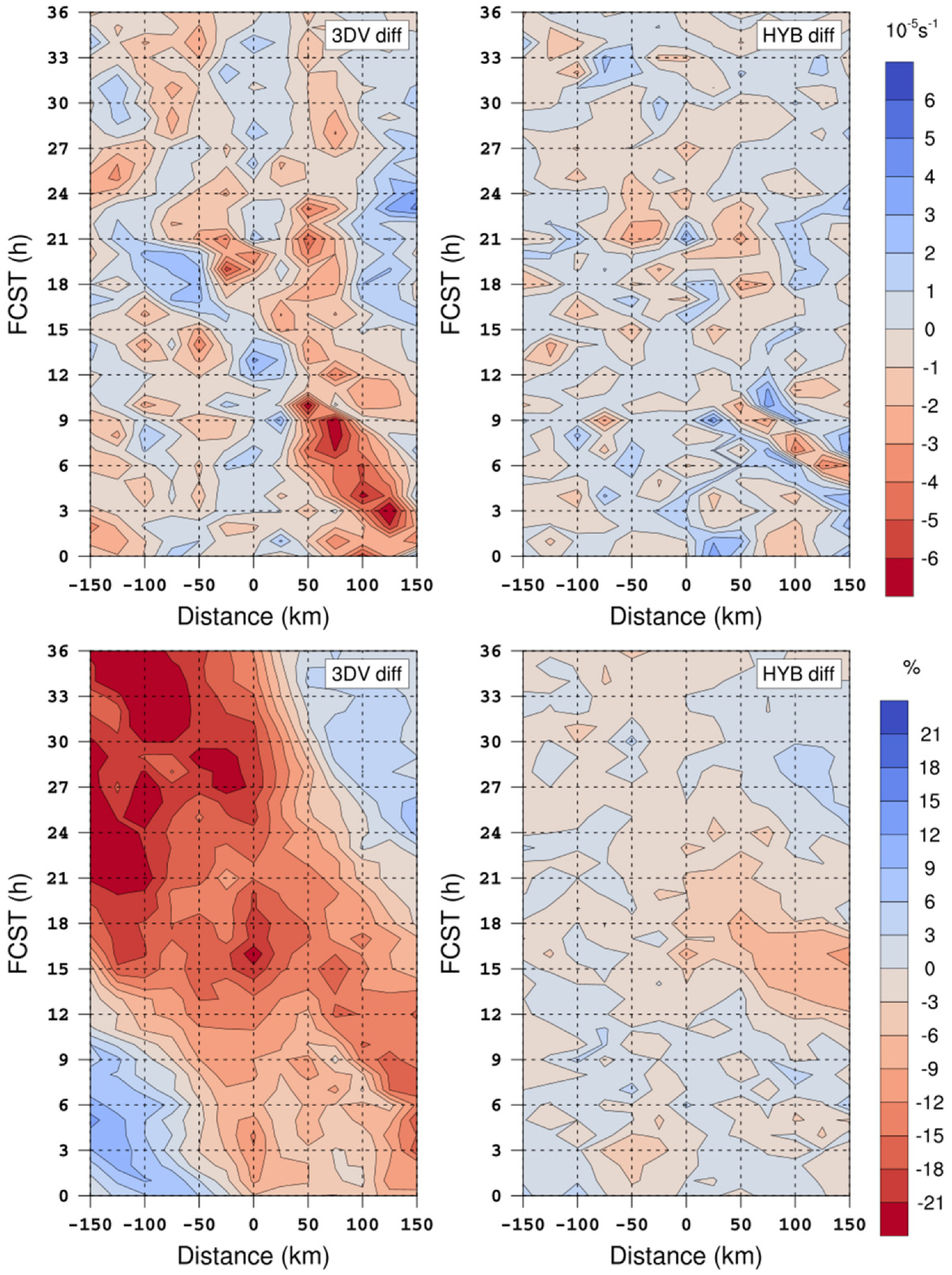
3.3. Modification Diagnosis

In order to analyze the modifications of precipitation simulations after radar DA, the Padang radar reflectivity data were used to calculate observation departure from the CTL and 3DV initial conditions at 00 h, namely, the O-B and O-A diagnostic fields. The 3DV departure (O-A) is the accumulation of hourly modifications from −03 h to 00 h. The composite radar reflectivity (the highest reflectivity at all of the elevations) observations at 00 h in each case, together with the calculated O-B and O-A fields, are exhibited in Figure 8. The topographic blocking from the coastal Barisan mountains was apparent, and useful landside samples after data quality control were hardly available in Cases 2–4. The decrease in coastal underestimation was noticeable in each case, in agreement with the 3DV improvements of precipitation simulation.
Figure 9 shows the relative humidity and vertical motion at 700 hPa and 500 hPa from the CTL and 3DV experiments averaged in Cases 1–4, where the few radar data samples around 850 hPa resulted in minor modifications of moist convection at the corresponding height. In Case 1, the precipitation probably occurred at around 700 hPa, where the convections had shapes which were consistent with precipitation. Stronger vertical motion and higher humidity were favorable for increased precipitation, which was sustained at the higher level of around 500 hPa. The increments of humidity and wind in the mountainous areas hardly led to any apparent improvements in the precipitation prediction. The enhancement of moisture and vertical transport was unidentifiable in Case 2, the case with the least improvement in the precipitation simulation. The assimilation impacts in Cases 3 and 4 were noticeable at 500 hPa, and their consistency with precipitation improvements suggests that precipitation took place at higher levels than in Case 1. These comparisons, with and without assimilation, indicate the positive influence of radar data assimilation on moist convection and precipitation.

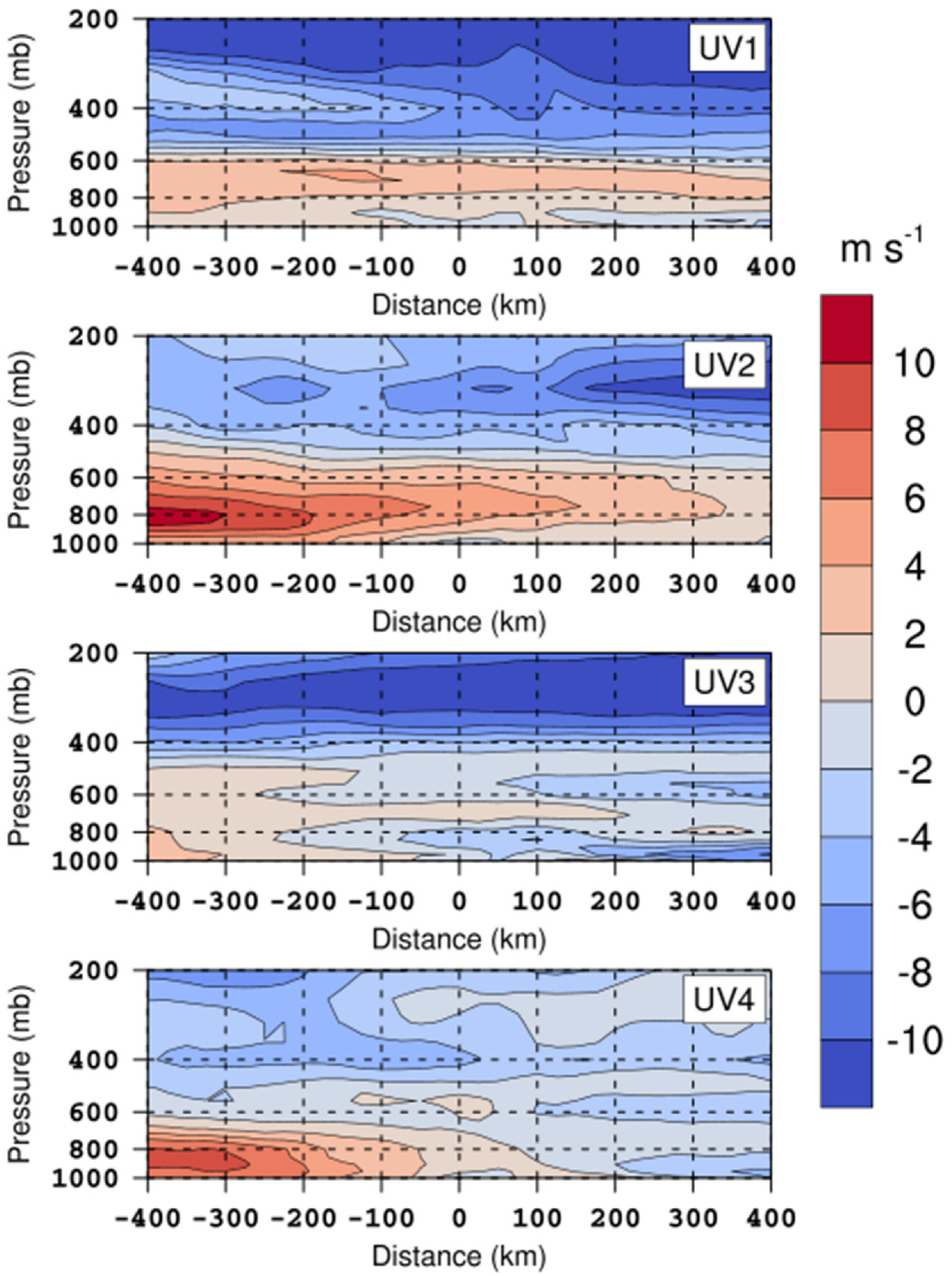
3.4. Synoptic Analysis

In order to further analyze the differences among the cases in terms of CTL behaviors and 3DV impacts, including the reason for the minor improvements in convection and precipitation after assimilation in Case 2, we looked at the large-scale synoptic background. Figure 10 shows the FNL coast-normal horizontal wind in the different cases. Low-level onshore wind, as well as a coastal land surge, is visible in most cases. Note that the offshore/onshore migration of precipitation is one of the diurnal features in MC coastal regions, but the direction of migration is not always the same as the direction of the low-level background wind, because other factors, such as gravity waves generated from the land-sea contrast or local-scale convection, could also have impacts [53,54,55,56].
Cases 2 and 4 were under the control of a stronger low-level onshore wind from the northern Indian Ocean, in contrast to Cases 1 and 3, where noticeable seaward migration of precipitation was generated under a weaker onshore wind and a stronger land surge. The WRF CTL simulations performed better in Cases 2 and 4, while poorer behavior in Cases 1 and 3 reflects the difficulties in describing topographic influences on convection and precipitation development, including seaside underestimation near the coastal Barisan mountains in Case 1, and overestimation around the mountains in Case 3. In other words, the WRF model could reasonably reproduce convection under stronger large-scale synoptic impacts, while its prediction of local-scale seaside convection and migration was easily ruined by other local factors, such as the model’s poor response to topography.
The observation departure (Figure 8) revealed visible seaside modifications of convection at initial conditions after radar data assimilation in Cases 2 and 4. However, the improvements of subsequent convection and precipitation from 3DV were apparently minor in Case 2. A possible explanation is the strong dilution of synoptic forcing. Under the background of an MJO active phase, the onshore wind was strongest in Case 2 and dominated from the surface to around 600 hPa. The strengthened landside advection and deep convection, as the main factor of precipitation in this case, easily overlapped the modifications from the data assimilation. This is distinguished from Case 4 where local-scale middle-level land surge and convection also largely modulated the precipitation, creating more favorable conditions for the assimilation effects to be sustained. On the other hand, no radar data assimilation was conducted farther offshore to modify the simulation of strengthened vapor advection from the northern Indian Ocean, as the dominant factor of precipitation in Case 2. Therefore, under strong large-scale forcing, such as an MJO active phase, assimilation of upper-stream observation is necessary to predict deep convection and heavy precipitation downstream.
The low-level synoptic features in Cases 1 and 3 reflected weaker impacts from seaside advection and stronger impacts from the local-scale land surge and convection; meanwhile, the 3DV improvements of the seaside precipitation prediction were more noticeable than in Case 2, reflecting a better influence of assimilation under a weaker large-scale synoptic background. The landside improvements under the unfavorable condition of few landside radar samples were noticeable, indicating that DA improvements could extend upstream and enhance the WRF model’s response to coastal topography. The abundant radar samples in Case 4 reflected stronger convection in a larger area compared with other cases; meanwhile the background westerly wind was not so strong as to heavily dilute the assimilation modifications. Therefore, the improvement in the precipitation simulation in Case 4 is outstanding.

3.5. Comparison between 3DVAR and 3DEnVAR Experiment

Besides the 4 short-term cases with hourly radar data assimilation from −03 h to 00 h before simulation, a longer period containing the duration of Case 3 was investigated, designated as Case 5, as indicated in Table 1. This case was controlled by a noticeable low-level land surge and local-scale convection (Figure 10), which was favorable for the sustained impacts of radar data assimilation. The forecasts in Case 5, using both the 3DV and HYB assimilation method, were validated and analyzed.
Figure 11 displays the hourly precipitation rates from the IMERG data and different WRF experiments. The seaward migration at the former 18 h and latter 18 h was revealed in IMERG, while the CTL simulation overestimated the former and underestimated the latter. In the CTL experiment, precipitation was generally overestimated during the 1st migration, especially at 09 h~15 h, and the underestimation during the 2nd migration was most noticeable at 27 h~33 h. Both the 3DV and HYB experiments reduced the CTL overestimation in the 1st migration, where the reduction in 3DV was slightly higher. The differences between 3DV and HYB came largely from the 2nd migration, which was very obscured in 3DV but was nicely caught in HYB, with an enhanced performance at 27 h~33 h compared with CTL.
The diagnostic fields of low-level moist convection are compared through differences in 850-hPa convergence and relative humidity in the 3DV and HYB experiments from those in the CTL experiment (Figure 12). As shown in the latter half of the 3DV experiment, weakened seaside convergence and humidity were unfavorable for vertical vapor transport, related to the obscured seaward migration. This phenomenon probably arose from the weakened landside convection and humidity during the earliest hours, aimed at reducing the overprediction of landside precipitation. However, as shown in Figure 11, in the CTL experiment the landside convection also moved seaward and triggered coastal convection during the latter half of the case, under the control of easterly land surges (Figure 10). Therefore, in the 3DV experiment, the severe cut in initial landside convection and the associated vertical vapor transport accumulated progressively and gradually influenced the following seaward migration. On the other hand, the HYB modifications within the earliest hours were relatively more neutral, and the reduction of moist convection afterward was not as severe as that in 3DV. As a result, the HYB experiment reasonably reproduced the 2nd migration of precipitation.
In general, under a 1- or 2-day assimilation cycle and simulation, the HYB method reached a better balance of positively influencing precipitation throughout the whole simulation, reflecting its advantage of more properly weighting the simulations and observations. Though further investigation with more cases is needed to prove whether this feature is common, the findings still reveal the potential superiority of the HYB assimilation method in leading to better model performance when hourly radar data assimilation is impossible due to low temporal resolution and only 6-hourly assimilation can be conducted.

4. Discussion

Numerous previous studies have revealed unsatisfying precipitation modeling in the MC, with reasons including the following: less coherent convective response under coarser model resolutions [55], a drier humidity reference profile in the parameterized cumulus convection [57], a lowered predictability of MC convection via a phase bias [58], and a potential dry bias within the input reanalysis data [59]. With respect to the analysis above, in this study the explicitly resolved convection under the cloud-permitting model resolution (3 km) instead of the parameterized convection, as well as conventional and radar data assimilation, helped the WRF model to reproduce precipitation more reasonably (Figure 6 and Figure 7). On the other hand, several data assimilation studies have focused on Sumatra, but they usually used radiosonde data [60,61] or satellite data [62,63]. Some other studies have used radar reflectivity data in order to estimate precipitation rates through semi-theoretical relationships [53,64,65], but few experiments assimilating radar data have been conducted on Sumatra or even in the MC. Therefore, this study is expected to represent pilot research to examine the influence of radar data assimilation on high-resolution numerical simulations during different MJO stages over the MC region.
The improvements with radar data assimilation come largely from the modifications of moisture conditions and wind structure [66,67,68,69], which are also revealed in this study. Note that most of the CDR reflectivity samples obtained at Padang exceeded 15 dBZ, while other samples generally within 15 dBZ were filtered off during the quality control. Gao et al. [70] defined a limit of 5 dBZ as no-rain echoes and found its assimilation to further reduce the bias and false alarm ratio of precipitation in the Colorado Rocky Mountains. Similar experiments in our study region might be worthwhile, for example during Case 1, where coastal underestimation north of Siberut island was turned into non-negligible overestimation after radar DA. Further improvement in the no-rain reflectivity assimilation is expected for WRF’s behavior in coastal topography, such as that of western Sumatra, and not only during heavy precipitation (e.g., Case 4) where abundant radar data samples guarantee the extent of DA impacts. In addition, during Case 5 the CTL experiment overestimated coastal precipitation in the former half (Figure 11), where improvements from 3DV DA and HYB DA were similar to each other (slightly better in 3DV). The main difference between the two DA experiments occurred in the latter half, where the seaward migration of CTL precipitation was hardly caught. The comparison supports the potential superiority of the HYB method over the 3DV method in terms of properly weighting background fields and observations, consistent with the findings of some previous research [40,69].

5. Conclusions

Based on the WRF model and the 3DVAR/hybrid 3DEnVAR method in the GSI data assimilation system, the present work assimilated radar reflectivity and radial velocity data to improve WRF’s initial conditions for high-resolution precipitation simulations during four 6-h cases and a 36-h case under different phases of an MJO event during January–February 2018. The radar data were obtained by a ground-based C-band Doppler radar located at Padang, Indonesia, a station on the west coast of Sumatra. IMERG precipitation products were utilized for the validation of the CTL, 3DVAR, and hybrid 3DEnVAR simulations. The modifications from assimilation were analyzed via observation departure in GSI analysis and modifications of convection properties. The major conclusions are summarized as follows:
Positive influences on 6-h precipitation simulations from the radar data assimilation were commonly visible in the coastal region. The diagnostic fields of moist convection were modified to reduce observation departures from the simulations. The radar data assimilation noticeably improved local-scale convection and migration but hardly influenced large-scale deep convection driven by a strong synoptic background, such as an MJO active phase. Under a 1- or 2-day assimilation cycle and simulation, the hybrid 3DEnVAR method reached a better balance of positively influencing precipitation throughout the whole simulation, as an advantage over the 3DVAR method, which focused on the earliest hours but found it difficult to catch the convection developments afterward.
Despite the results showing the positive impacts of radar data assimilation on the numerical simulations, more work needs to be done in future studies. Since single-radar observations have limited coverage, simulation improvements could be enhanced if multiple radar observations were available. Therefore, more studies using numerous radar datasets with broader coverage are needed for more significant improvements in modeling and further confirmation of current findings. Also, since this paper presents a pilot study to examine the influences of radar data assimilation on high-resolution numerical simulations over the MC region, more advanced remote-sensing data assimilation techniques should be used, including applying the hybrid 3DEnVAR method more widely. In addition, the capability of high-resolution numerical models to catch the generation of local convection in western Sumatra during different strong synoptic backgrounds still needs to be enhanced.

Author Contributions

Conceptualization, B.Z., Z.P. and Z.G.; methodology, B.Z. and Z.P.; data curation: Z.P. and A.W.P.; software, B.Z. and Z.P.; validation, B.Z., Z.P. and Z.G.; formal analysis, B.Z. and Z.P.; writing—original draft preparation, B.Z.; writing—review and editing, B.Z., Z.P. and Z.G.; visualization, B.Z.; supervision, Z.P. and Z.G.; funding acquisition, Z.P. and A.W.P. All authors have read and agreed to the published version of the manuscript.

Funding

The authors Z.P. and A.W.P. were supported by NOAA (Award NA17OAR4310262).

Institutional Review Board Statement

Not applicable.

Informed Consent Statement

Not applicable.

Data Availability Statement

The MJO RMM index data were from the Australian Bureau of Meteorology (http://www.bom.gov.au/climate/mjo/; accessed on 1 February 2021). The NCEP GDAS/FNL Analysis data as well as the ADP global upper-air and surface weather observations were from the Research Data Archive at the National Center for Atmospheric Research, Computational and Information Systems Laboratory (https://doi.org/10.5065/D65Q4T4Z; https://doi.org/10.5065/Z83F-N512; accessed on 10 February 2021). The NCEP GFS global EnKF 80 ensemble members data were obtained from the NCEP Global Ensemble Forecast System (accessed on 1 February 2021). The radar reflectivity data and radial velocity data were originally from the Meteorology, Climatology, and Geophysical Agency (BMKG), Indonesia (accessed on 15 February 2021). The IMERG precipitation data were from NASA′s Global Precipitation Measurement Mission (https://gpm.nasa.gov/data/imerg; accessed on 10 February 2021). The ISD precipitation data were obtained from NCEI (https://www.ncei.noaa.gov; accessed on 10 October 2021).

Acknowledgments

The authors acknowledge Courtney Schumacher from Texas A&M University for her help in processing the radar data quality control and her early comments on this study. The first author (B.Z.) worked at the University of Utah during 2018–2020 under scholarship support from the Chinese Scholar Council during this study. The authors Z.P. and A.W.P. were supported by the NOAA YMC program with Grant #NA17OAR4310262. The author Z.G. was supported by the National Natural Science Foundation of China (Grant: 42175082). Computer support from the Center for High-Performance Computing at the University of Utah is gratefully acknowledged.

Conflicts of Interest

The authors declare no conflict of interest.

References

  1. Katsumata, M.; Mori, S.; Hamada, J.-I.; Hattori, M.; Syamsudin, F.; Yamanaka, M.D. Diurnal cycle over a coastal area of the maritime continent as derived by special networked soundings over Jakarta during HARIMAU2010. Prog. Earth Planet. Sci. 2018, 5, 64. [Google Scholar] [CrossRef]
  2. Mori, S.; Hamada, J.-I.; Hattori, M.; Wu, P.-M.; Katsumata, M.; Endo, N.; Ichiyanagi, K.; Hashiguchi, H.; Arbain, A.A.; Sulistyowati, R.; et al. Meridional march of diurnal rainfall over Jakarta, Indonesia, observed with a C-band doppler radar: An overview of the HARIMAU2010 campaign. Prog. Earth Planet. Sci. 2018, 5, 47. [Google Scholar] [CrossRef]
  3. Neale, R.; Slingo, J. The maritime continent and its role in the global climate: A GCM study. J. Clim. 2003, 16, 834–848. [Google Scholar] [CrossRef]
  4. Chang, C.-P.; Harr, P.A.; Chen, H.-J. Synoptic disturbances over the equatorial South China sea and Western maritime continent during Boreal winter. Mon. Weather Rev. 2005, 133, 489–503. [Google Scholar] [CrossRef]
  5. Lorenz, P.; Jacob, D. Influence of regional scale information on the global circulation: A two-way nesting climate simulation. Geophys. Res. Lett. 2005, 32, L18706. [Google Scholar] [CrossRef] [Green Version]
  6. Ando, K.; Syamsudin, F.; Ishihara, Y.; Pandoe, W.; Yamanaka, M.D.; Masumoto, Y.; Mizuno, K. Development of new international research laboratory for maritime-continent seas climate research and contributions to global surface moored buoy array. In Proceedings of the OeanObs’09: Sustained Ocean Observations and Information for Society Conference (Annex), Venice, Italy, 21–25 September 2009. [Google Scholar]
  7. Madden, R.A.; Julian, P.R. Detection of a 40–50 day oscillation in the zonal wind in the tropical Pacific. J. Mospheric Sci. 1971, 28, 702–708. [Google Scholar] [CrossRef]
  8. Madden, R.A.; Julian, P.R. Description of global-scale circulation cells in the tropics with a 40–50 day period. J. Atmos. Sci. 1972, 29, 1109–1123. [Google Scholar] [CrossRef]
  9. Zhang, C. Madden-julian oscillation. Rev. Geophys. 2005, 43, RG2003. [Google Scholar] [CrossRef] [Green Version]
  10. Barrett, B.S.; Carrasco, J.; Testino, A.P. Madden-Julian Oscillation (MJO) modulation of atmospheric circulation and chilean winter precipitation. J. Clim. 2012, 25, 1678–1688. [Google Scholar] [CrossRef]
  11. Jeong, J.-H.; Kim, B.-M.; Ho, C.-H.; Noh, Y.-H. Systematic variation in wintertime precipitation in East Asia by MJO-induced extratropical vertical motion. J. Clim. 2008, 21, 788–801. [Google Scholar] [CrossRef]
  12. Juliá, C.; Rahn, D.A.; Rutllant, J.A. Assessing the influence of the MJO on strong precipitation events in subtropical, semi-arid north-central Chile (30°S). J. Clim. 2012, 25, 7003–7013. [Google Scholar] [CrossRef] [Green Version]
  13. Zhang, C.; Ling, J. Barrier Effect of the Indo-Pacific Maritime Continent on the MJO: Perspectives from Tracking MJO Precipitation. J. Clim. 2017, 30, 3439–3459. [Google Scholar] [CrossRef]
  14. Zhou, S.; L’Heureux, M.; Weaver, S.; Kumar, A. A composite study of the MJO influence on the surface air temperature and precipitation over the Continental United States. Clim. Dyn. 2011, 38, 1459–1471. [Google Scholar] [CrossRef]
  15. Kim, H.-M.; Webster, P.J.; Toma, V.E.; Kim, D. Predictability and prediction skill of the MJO in two operational forecasting systems. J. Clim. 2014, 27, 5364–5378. [Google Scholar] [CrossRef]
  16. Kim, H.-M.; Kim, D.; Vitart, F.; Toma, V.E.; Kug, J.-S.; Webster, P.J. MJO propagation across the Maritime Continent in the ECMWF ensemble prediction System. J. Clim. 2016, 29, 3973–3988. [Google Scholar] [CrossRef]
  17. Liu, X.; Wu, T.; Yang, S.; Li, T.; Jie, W.; Zhang, L.; Wang, Z.; Liang, X.; Li, Q.; Cheng, Y.; et al. MJO prediction using the sub-seasonal to seasonal forecast model of Beijing Climate Center. Clim. Dyn. 2016, 48, 3283–3307. [Google Scholar] [CrossRef] [Green Version]
  18. Vintzileos, A.; Pan, H.-L. On the Importance of Horizontal Resolution and Initial Conditions to Forecasting Tropical Intraseasonal Oscillations: The Maritime Continent Prediction Barrier. Available online: http://www.nws.noaa.gov/ost/climate/STIP/CTB-COLA/Augustin_091907.htm (accessed on 28 June 2020).
  19. Gao, J.; Stensrud, D.J. Assimilation of reflectivity data in a convective-scale, cycled 3dvar framework with hydrometeor classification. J. Atmos. Sci. 2012, 69, 1054–1065. [Google Scholar] [CrossRef]
  20. Lai, A.; Min, J.; Gao, J.; Ma, H.; Cui, C.; Xiao, Y.; Wang, Z. Assimilation of Radar Data, Pseudo Water Vapor, and Potential Temperature in a 3DVAR Framework for Improving Precipitation Forecast of Severe Weather Events. Atmosphere 2020, 11, 182. [Google Scholar] [CrossRef] [Green Version]
  21. Radhakrishnan, C.; Chandrasekar, V. CASA Prediction System over Dallas-Fort Worth Urban Network: Blending of Nowcasting and High-Resolution Numerical Weather Prediction Model. J. Atmos. Ocean. Technol. 2020, 37, 211–228. [Google Scholar] [CrossRef]
  22. L’Heureux, M. The Madden Julian Oscillation has been active so far this winter. Here is why it matters. ENSO Blog 2018, 22. Available online: https://www.climate.gov/news-features/blogs/enso/madden-julian-oscillation-has-been-active-so-far-winter-here-why-it (accessed on 22 June 2020).
  23. Wheeler, M.C.; Hendon, H.H. An all-season real-time multivariate MJO index: Development of an index for monitoring and prediction. Mon. Weather Rev. 2004, 132, 1917–1932. [Google Scholar] [CrossRef]
  24. Wei, Y.; Pu, Z.; Zhang, C. Diurnal cycle of precipitation over the Maritime Continent under modulation of MJO: Perspectives from cloud-permitting scale simulations. J. Geophys. Res. Atmos. 2020, 125, e2020JD032529. [Google Scholar] [CrossRef]
  25. Zhao, K.; Xue, M. Assimilation of coastal Doppler radar data with the ARPS 3DVAR and cloud analysis for the prediction of Hurricane Ike (2008). Geophys. Res. Lett. 2009, 36, L12803. [Google Scholar] [CrossRef] [Green Version]
  26. Stensrud, D.J.; Gao, J. Importance of horizontally inhomogeneous environmental initial conditions to ensemble storm-scale radar data assimilation and very short-range forecasts. Mon. Weather Rev. 2010, 138, 1250–1272. [Google Scholar] [CrossRef]
  27. Schenkman, A.D.; Xue, M.; Shapiro, A.; Brewster, K.; Gao, J. The analysis and prediction of the 8–9 May 2007 Oklahoma tornadic mesoscale convective system by assimilating WSR-88D and CASA radar data using 3DVAR. Mon. Weather Rev. 2011, 139, 224–246. [Google Scholar] [CrossRef] [Green Version]
  28. Jones, T.A.; Knopfmeier, K.; Wheatley, D.; Creager, G.; Minnis, P.; Palikonda, R. Storm-scale data assimilation and en-semble forecasting with the NSSL experimental Warn-on-Forecast system. Part II: Combined radar and satellite data experiments. Weather Forecast. 2016, 31, 297–327. [Google Scholar] [CrossRef]
  29. Yussouf, N.; Kain, J.S.; Clark, A.J. Short-term probabilistic forecasts of the 31 May 2013 Oklahoma tornado and flash flood event using a continuous-update-cycle storm-scale ensemble system. Weather Forecast. 2016, 31, 957–983. [Google Scholar] [CrossRef]
  30. Skamarock, W.C.; Klemp, J.B.; Dudhia, J.; Gill, D.O.; Liu, Z.; Berner, J.; Wang, W.; Powers, J.G.; Duda, M.G.; Barker, D.M. A Description of the Advanced Research WRF Model Version 4; National Center for Atmospheric Research: Boulder, CO, USA, 2019; Volume 145, p. 145. [Google Scholar]
  31. National Centers for Environmental Prediction/National Weather Service/NOAA/U.S. Department of Commerce. 2015, Updated Daily. NCEP GDAS/FNL 0.25 Degree Global Tropospheric Analyses and Forecast Grids. Research Data Archive at the National Center for Atmospheric Research, Computational and Information Systems Laboratory. Available online: https://rda.ucar.edu/datasets/ds083.3/ (accessed on 10 October 2018). [CrossRef]
  32. Hong, S.-Y.; Lim, J.-O.J. The WRF single-moment 6-class microphysics scheme (WSM6). Asia Pac. J. Atmos. Sci. 2006, 42, 129–151. [Google Scholar]
  33. Iacono, M.; Delamere, J.S.; Mlawer, E.J.; Shephard, M.W.; Clough, S.A.; Collins, W. Radiative forcing by long-lived greenhouse gases: Calculations with the AER radiative transfer models. J. Geophys. Res. Space Phys. 2008, 113, D13103. [Google Scholar] [CrossRef]
  34. Hong, S.-Y.; Noh, Y.; Dudhia, J. A new vertical diffusion package with an explicit treatment of entrainment processes. Mon. Weather Rev. 2006, 134, 2318–2341. [Google Scholar] [CrossRef] [Green Version]
  35. Grell, G.A.; Dudhia, J.; Stauffer, D.R. A Description of the Fifth-Generation Penn State/NCAR Mesoscale Model (MM5); No. NCAR/TN-398+STR; University Corporation for Atmospheric Research: Boulder, CO, USA, 1994. [Google Scholar]
  36. Chen, F.; Dudhia, J. Coupling an advanced land surface–hydrology model with the Penn State–NCAR MM5 modeling system. Part I: Model implementation and sensitivity. Mon. Weather Rev. 2001, 129, 569–585. [Google Scholar] [CrossRef] [Green Version]
  37. Zhang, C.; Wang, Y. Projected Future Changes of Tropical Cyclone Activity over the Western North and South Pacific in a 20-km-Mesh Regional Climate Model. J. Clim. 2017, 30, 5923–5941. [Google Scholar] [CrossRef]
  38. Developmental Testbed Center. 2016: Gridpoint Statistical Interpolation Advanced User’s Guide Version 3.5.0.0. Available online: https://dtcenter.org/community-code/gridpoint-statistical-interpolation-gsi/documentation (accessed on 14 November 2018).
  39. Wu, W.-S.; Purser, R.J.; Parrish, D.F. Three-dimensional variational analysis with spatially inhomogeneous covariances. Mon. Weather Rev. 2002, 130, 2905–2916. [Google Scholar] [CrossRef] [Green Version]
  40. Gao, J.; Xue, M.; Stensrud, D.J. The development of a hybrid EnKF-3DVAR algorithm for storm-scale data assimilation. Adv. Meteorol. 2013, 2013, 512656. [Google Scholar] [CrossRef] [Green Version]
  41. Fisher, M. Background error covariance modelling. In Proceedings of the Seminar on Recent Development in Data Assimilation for Atmosphere and Ocean, Shinfield Park, Reading, UK, 8–12 September 2003; pp. 45–63. [Google Scholar]
  42. Pu, Z.; Kalnay, E. Numerical weather prediction basics: Models, numerical methods, and data assimilation. In Handbook of Hydro meteorological Ensemble Forecasting; Springer: Berlin, Germany, 2019; pp. 1–31. [Google Scholar]
  43. Zhou, X.; Zhu, Y.; Hou, D.; Luo, Y.; Peng, J.; Wobus, R. Performance of the new NCEP Global Ensemble Forecast System in a parallel experiment. Weather Forecast. 2017, 32, 1989–2004. [Google Scholar] [CrossRef]
  44. Wang, X. Incorporating ensemble covariance in the gridpoint statistical interpolation variational minimization: A mathematical framework. Mon. Weather Rev. 2010, 138, 2990–2995. [Google Scholar] [CrossRef] [Green Version]
  45. Hu, M.; Weygandt, S.; Xue, M.; Benjamin, S. Development and testing of a new cloud analysis package using radar, satellite, and surface cloud observations within GSI for initializing Rapid Refresh. In Proceedings of the 22nd Conference on Weather Analysis and Forecasting/18th Conference on Numerical Weather Prediction, Park City, UT, USA, 25–29 June 2007. [Google Scholar]
  46. Purser, R.J.; Parrish, D.F.; Masutani, M. Meteorological observational data compression; an alternative to conventional “super-obbing”. NCEP Office Note 2000, 430, 13. [Google Scholar]
  47. Liu, S.; Xue, M.; Gao, J.; Parrish, D. Analysis and impact of super-obbed Doppler radial velocity in the NCEP grid-point statistical interpolation (GSI) analysis system. In Proceedings of the 17th Conference on Numerical Weather Prediction, Washington DC, USA, 1–5 August 2005; p. 13A.4. [Google Scholar]
  48. National Centers for Environmental Prediction/National Weather Service/NOAA/U.S. Department of Commerce. 2008, Updated Daily. NCEP ADP Global Upper Air and Surface Weather Observations (PREPBUFR format). Research Data Archive at the National Center for Atmospheric Research, Computational and Information Systems Laboratory. Available online: https://rda.ucar.edu/datasets/ds337.0/ (accessed on 14 May 2020). [CrossRef]
  49. Huffman, G.J.; Bolvin, D.T.; Braithwaite, D.; Hsu, K.; Joyce, R.; Xie, P.; Yoo, S.-H. NASA global precipitation measurement (GPM) integrated multi-satellite retrievals for GPM (IMERG). Algorithm Theor. Basis Doc. (ATBD) Version 2015, 4, 26. [Google Scholar]
  50. Tan, J.; Huffman, G.J.; Bolvin, D.T.; Nelkin, E.J. IMERG V06: Changes to the morphing algorithm. J. Atmos. Ocean. Technol. 2019, 36, 2471–2482. [Google Scholar] [CrossRef]
  51. Roberts, N.M.; Lean, H.W. Scale-selective verification of rainfall accumulations from high-resolution forecasts of convective events. Mon. Weather Rev. 2008, 136, 78–97. [Google Scholar] [CrossRef]
  52. Smith, A.; Lott, N.; Vose, R.S. The integrated surface database: Recent developments and partnerships. Bull. Am. Meteorol. Soc. 2011, 92, 704–708. [Google Scholar] [CrossRef]
  53. Yokoi, S.; Mori, S.; Katsumata, M.; Geng, B.; Yasunaga, K.; Syamsudin, F.; Nurhayati; Yoneyama, K. Diurnal cycle of precipitation observed in the western coastal area of Sumatra Island: Offshore preconditioning by gravity waves. Mon. Weather Rev. 2017, 145, 3745–3761. [Google Scholar] [CrossRef]
  54. Mori, S.; Jun-Ichi, H.; Tauhid, Y.I.; Yamanaka, M.D.; Okamoto, N.; Murata, F.; Sakurai, N.; Hashiguchi, H.; Sribimawati, T. Diurnal land-sea rainfall peak migration over Sumatera Island, Indonesian Maritime Continent, observed by TRMM satellite and intensive rawinsonde soundings. Mon. Weather Rev. 2004, 132, 2021–2039. [Google Scholar] [CrossRef]
  55. Love, B.S.; Matthews, A.J.; Lister, G.M.S. The diurnal cycle of precipitation over the Maritime Continent in a high-resolution atmospheric model. Q. J. R. Meteorol. Soc. 2011, 137, 934–947. [Google Scholar] [CrossRef] [Green Version]
  56. Short, E.; Vincent, C.L.; Lane, T.P. Diurnal cycle of surface winds in the Maritime Continent observed through satellite scatterometry. Mon. Weather Rev. 2019, 147, 2023–2044. [Google Scholar] [CrossRef]
  57. Fonseca, R.M.; Zhang, T.; Yong, K.-T. Improved simulation of precipitation in the tropics using a modified BMJ scheme in the WRF model. Geosci. Model. Dev. 2015, 8, 2915–2928. [Google Scholar] [CrossRef] [Green Version]
  58. Wang, S.; Sobel, A.H.; Tippett, M.K.; Vitart, F. Prediction and predictability of tropical intraseasonal convection: Seasonal dependence and the Maritime Continent prediction barrier. Clim. Dyn. 2018, 52, 6015–6031. [Google Scholar] [CrossRef]
  59. Dipankar, A.; Webster, S.; Huang, X.-Y.; Doan, V.Q. Understanding biases in simulating the diurnal cycle of convection over the western coast of Sumatra: Comparison with pre-YMC observation campaign. Mon. Weather Rev. 2019, 147, 1615–1631. [Google Scholar] [CrossRef]
  60. Seto, T.H.; Tabata, Y.; Yamamoto, M.K.; Hashiguchi, H.; Mega, T.; Kudsy, M.; Yamanaka, M.D.; Fukao, S. Comparison Study of Lower-tropospheric Horizontal Wind over Sumatra, Indonesia Using NCEP/NCAR Reanalysis, Operational Radiosonde, and the Equatorial Atmosphere Radar. SOLA 2009, 5, 21–24. [Google Scholar] [CrossRef] [Green Version]
  61. Lee, J.C.K.; Dipankar, A.; Huang, X.-Y. On the Sensitivity of the Simulated Diurnal Cycle of Precipitation to 3-Hourly Radiosonde Assimilation: A Case Study over the Western Maritime Continent. Mon. Weather Rev. 2021, 149, 3449–3468. [Google Scholar]
  62. Shoji, Y.; Kunii, M.; Saito, K. Mesoscale data assimilation of Myanmar cyclone Nargis Part II: Assimilation of GPS-derived precipitable water vapor. J. Meteorol. Soc. Japan. Ser. II 2011, 89, 67–88. [Google Scholar] [CrossRef] [Green Version]
  63. Saragih, I.J.A.; Mukhsinin, H.A.; Tarigan, K.; Sinambela, M.; Situmorang, M.; Sembiring, K.; Humaidi, S. Improvement in WRF model prediction for heavy rain events over North Sumatra region using satellite data assimilation. IOP Conference Series: Earth and Environmental Science. In Proceedings of the 2nd International Conference on Tropical Meteorology and Atmospheric Sciences, Jakarta, Indonesia, 23–25 March 2021; p. 012040. [Google Scholar]
  64. Yokoi, S.; Mori, S.; Syamsudin, F.; Haryoko, U.; Geng, B. Environmental conditions for nighttime offshore migration of precipitation area as revealed by in situ observation off Sumatra Island. Mon. Weather Rev. 2019, 147, 3391–3407. [Google Scholar] [CrossRef]
  65. Bai, H.; Deranadyan, G.; Schumacher, C.; Funk, A.; Epifanio, C.; Ali, A.; Endarwin; Radjab, F.; Adriyanto, R.; Nurhayati, N. Formation of Nocturnal Offshore Rainfall near the West Coast of Sumatra: Land Breeze or Gravity Wave? Mon. Weather Rev. 2021, 149, 715–731. [Google Scholar] [CrossRef]
  66. Li, Z.; Pu, Z.; Sun, J.; Lee, W.-C. Impacts of 4DVAR assimilation of airborne Doppler Radar observations on numerical simulations of the genesis of Typhoon Nuri (2008). J. Appl. Meteorol. Clim. 2014, 53, 2325–2343. [Google Scholar] [CrossRef]
  67. Wang, H.; Wang, D.; WAN, Q. Application of assimilating Doppler weather radar data in the “7.21” Beijing excessive storm. Acta Meteorol. Sin. 2015, 73, 679–696. [Google Scholar]
  68. Lin, E.; Yang, Y.; Qiu, X.; Xie, Q.; Gan, R.; Zhang, B.; Liu, X. Impacts of the radar data assimilation frequency and large-scale constraint on the short-term precipitation forecast of a severe convection case. Atmos. Res. 2021, 257, 105590. [Google Scholar] [CrossRef]
  69. Shen, F.; Min, J.; Xu, D. Assimilation of radar radial velocity data with the WRF Hybrid ETKF-3DVAR system for the prediction of Hurricane Ike (2008). Atmos. Res. 2016, 169, 127–138. [Google Scholar] [CrossRef]
  70. Gao, S.; Sun, J.; Min, J.; Zhang, Y.; Ying, Z. A scheme to assimilate “no rain” observations from Doppler radar. Weather Forecast. 2018, 33, 71–88. [Google Scholar] [CrossRef]
Figure 1. MJO RMM phase diagram for January (blue)–February (green) 2018 with locations of the 4 6-h cases attached.
Remotesensing 14 00042 g001
Figure 2. Terrain height (m) in the WRF domain. The black cross and red circle mark the Padang radar location and data coverage. The orange dots mark the ISD sites Tabing (0.9°S, 100.4°E) and Japura Airport (0.4°S, 102.3°E). The solid black box marks the transect used for the Hovmöller diagrams (Figures 10–12).
Remotesensing 14 00042 g002
Figure 3. Illustrations of the experiments in different cases.
Remotesensing 14 00042 g003
Figure 4. Padang radar reflectivity (shaded, dBZ) and IMERG precipitation rate (contours, >1 mm/h in Case 3 and >3 mm/h in other cases) during 01 h–06 h in Cases 1–4. The CxTy in the panels indicates the yth hour of Case x.
Remotesensing 14 00042 g004
Figure 5. Statistics of PCC, BIAS, and RMSE from ISD and IMERG hourly precipitation (mm h−1) at (a) Tabing and (b) Japura Airport during January and February 2018. The PCC values are significant at the 0.01 level according to the Student′s t-test (marked with “**”).
Remotesensing 14 00042 g005
Figure 6. Accumulated precipitation (mm) from IMERG (IMG), CTL simulation, and 3DV simulation during Cases 1–4. The numbers included in the panels indicate the corresponding case number.
Remotesensing 14 00042 g006
Figure 7. FSS scores for the CTL and 3DV experiments in Cases 1–4. The numbers included in the panels indicate the corresponding case number.
Remotesensing 14 00042 g007
Figure 8. (Left) Composite radar reflectivity observations and departure from the (middle) CTL simulation and (right) 3DV simulation at 00 h in Cases 1–4. The numbers included in the panels indicate the corresponding case number.
Remotesensing 14 00042 g008
Figure 9. Relative humidity (shaded, %) and >0.05 m/s vertical motion (shaded) at 700 hPa and 500 hPa averaged from the CTL and 3DV experiments during Cases 1–4. The numbers in the panels indicate the corresponding case numbers.
Remotesensing 14 00042 g009
Figure 10. Vertical cross sections of coast-normal horizontal wind (positive onshore) during Cases 1–4 from FNL data averaged in the solid black transect shown in Figure 2. The distance dimension is along the longer side of the transection, with positive (negative) distance on the land (sea) side. The numbers in the panels indicate the corresponding case numbers.
Remotesensing 14 00042 g010
Figure 11. Hovmöller diagrams of hourly precipitation rate from IMERG data and WRF experiments (CTL, 3DV, HYB) during Case 5, averaged in the solid black transect shown in Figure 2.
Remotesensing 14 00042 g011
Figure 12. Hovmöller diagrams of 850-hPa differences in convergence (10−5 s−1, above) and relative humidity (%, below) in the 3DV and HYB experiments during Case 5 with CTL simulations subtracted, averaged in the solid black transect shown in Figure 2.
Remotesensing 14 00042 g012
Table 1. Durations of different cases and configurations of radar data assimilation.
Case ConfigurationAssimilation:
General Configuration
Assimilation:
Super-ob Configuration
Case NumberStarting TimeEnding TimeSpin-UpDurationHalf Time WindowAzimuth Angle IntervalElevation Angle IntervalRadial Distance IntervalObservation Density Threshold
Case 11500 UTC
7 January 2018
2100 UTC
7 January 2018
−15 h~−03 h−03 h~00 h
hourly
0.5 h0.25°5 km30
Case 20000 UTC
24 January 2018
0600 UTC
24 January 2018
Case 32100 UTC
11 February 2018
0300 UTC
12 February 2018
Case 41800 UTC
22 February 2018
0000 UTC
23 February 2018
Case 51200 UTC
11 February 2018
0000 UTC
13 February 2018
−24 h~−12 h−12 h~30 h
6-hourly
1 h
Publisher’s Note: MDPI stays neutral with regard to jurisdictional claims in published maps and institutional affiliations.

