Article

Comparison of Macro- and Microphysical Properties in Precipitating and Non-Precipitating Clouds over Central-Eastern China during Warm Season

1
Anhui Weather Modification Office, Hefei 230031, China
2
Climate and Weather Disasters Collaborative Innovation Center, Key Laboratory for Aerosol-Cloud-Precipitation of China Meteorological Administration, School of Atmospheric Physics, Nanjing University of Information Science and Technology, Nanjing 210044, China
*
Author to whom correspondence should be addressed.
Remote Sens. 2022, 14(1), 152; https://doi.org/10.3390/rs14010152
Submission received: 31 October 2021 / Revised: 25 December 2021 / Accepted: 25 December 2021 / Published: 30 December 2021

Abstract

:
The macro- and microphysical properties of clouds can reflect their vertical physical structure and evolution and are important indications of the formation and development of precipitation. We used four-year merged CloudSat-CALIPSO-MODIS products to distinguish the macro- and microphysical properties of precipitating and non-precipitating clouds over central-eastern China during the warm season (May–September). Our results showed that the clouds were dominated by single- and double-layer forms with occurrence frequencies > 85%. Clouds with a low probability of precipitation (POP) were usually geometrically thin. The POP showed an increasing trend with increases in the cloud optical depth, liquid water path, and ice water path, reaching maxima of 50%, 60%, and 75%, respectively. However, as cloud effective radius (CER) increased, the POP changed from an increasing to a decreasing trend for a CER > 22 μm, in contrast with our perception that large particles fall more easily against updrafts, but this shift can be attributed to the transition of the cloud phase from mixed clouds to ice clouds. A high POP > 60% usually occurred in mixed clouds with vigorous ice-phase processes. There were clear differences in the microphysical properties of non-precipitating and precipitating clouds. In contrast with the vertical evolution of non-precipitating clouds with weaker reflectivity, precipitating clouds were present above 0 dBZ with a significant downward increase in reflectivity, suggesting inherent differences in cloud dynamical and microphysical processes. Our findings highlight the differences in the POP of warm and mixed clouds, suggesting that the low frequency of precipitation from water clouds should be the focus of future studies.

1. Introduction

Clouds are key components of the Earth’s climate system and have a crucial role in modulating the radiation budget and hydrological cycle [1,2]. The extent to which they do so depends on a variety of cloud parameters, including macro-physical (e.g., occurrence frequency, cloud height, geometric thickness) and microphysical (e.g., optical depth, effective radius, water path, etc.) properties [2,3]. These parameters have been introduced in previous studies. The effective radius is the area-weighted mean radius of cloud droplets, which is proportional to the ratio of the volume of cloud droplets to the projected area [4]. Cloud optical depth is derived from the full integration of radiation attenuation through the clouds, indicating the cloud opacity at specific wavelengths [5]. Quantitative assessment of liquid water content, which is an integration over the mass of cloud droplet size distribution, could provide the information of cloud water distribution [4]. In fact, these basic parameters are intimately related with each other and linked with droplet number concentration and size distribution [4,6], a large change in effective radius could be due to a small variation in droplet number concentration for a given liquid water content [7]. Small changes in values of cloud properties and their variability in the horizontal and vertical can result in striking differences in the effects of clouds on climate [8,9,10].
Providing information about the vertical variation of cloud properties has a significant impact not only on radiation processes, but also on precipitation processes [11,12]. The vertical characteristics of clouds influence atmospheric heating and thus affect global atmospheric energy transport by modulating the amount of energy reflected, emitted, and absorbed at the surface and in the atmosphere [13]. The contribution of different cloud systems to the radiative heating of the atmosphere has been the subject of several studies, on the global annual mean, clouds induce a net planetary atmospheric radiative heating of 0.07 ± 0.08 K day−1 [13,14]. Particularly, precipitation is important in contributing heat budget through the release of latent heat during hydrometeor formation and growth [15,16]. Nelson et al. [17] estimated the global character of latent heating in warm rain systems, and they found that net column-integrated latent heating from warm rain condensation contribute 0.15 K day−1 (7.44 W m−2) of atmospheric heating, with nearly equal contribution from convective and shallow warm rain. In addition, the vertical structure of clouds also influences microphysical processes such as collision and sedimentation, thereby affecting the occurrence and intensity of precipitation [18,19]. However, the description of cloud vertical structure contributes to one of the largest uncertainties in climate simulations and projections [12,20]. Therefore, the knowledge of vertical structure of different cloud types (both precipitating and non-precipitating) needs to be improved and is important for better cloud simulations in weather and climate models.
Satellite-based remote sensing observations have a crucial role in cloud studies given their advantages of continuous monitoring and wide coverage [21,22]. Conventional passive sensors provide abundant information near the cloud top, but they cannot adequately characterize the internal structure of the entire cloud column as a result of their limited penetration into clouds. By contrast, the operation of active sensors in space, such as the Cloud Profiling Radar (CPR) system on-board the CloudSat satellite [23] and the Cloud-Aerosol Lidar with Orthogonal Polarization (CALIOP) system on-board Cloud-Aerosol Lidar and Infrared Pathfinder Satellite Observations (CALIPSO) satellite [24], can compensate for the deficiencies of passive sensors.
Synergistic observations from the CPR and CALIOP instruments offer an unprecedented opportunity for a comprehensive analysis of the occurrence and vertical structure of thin to thick clouds [5,25]. For instance, Luo et al. [26] compared the distributions of hydrometeors in two Asian monsoon regions and found that the average hydrometeor occurrence frequency in eastern China was 80%, 10% higher than that in the Indian monsoon region. Das et al. [27] showed that the formation of thicker clouds is maintained by strong updrafts and high humidity. Kukulies et al. [28] confirmed the dominant role of low-level single-layer clouds over the Tibetan Pleateau, where there are daytime–nighttime differences in the frequency, vertical structure, and water path of cloud systems in the summer [29,30]. Overall, these studies are of great value in improving our knowledge of clouds on both regional and global scales. The 3D features of clouds from combined CloudSat–CALIPSO observations have been archived, and it is therefore possible to investigate in detail the linkage between clouds and precipitation. Gao et al. [31] demonstrated the growth processes from cloud particles to drizzle and raindrops within single-layer warm clouds over the northern hemisphere and showed that these processes are associated with an increase in the liquid water path (LWP). Kikuchi et al. [32] showed the systematic transition of deep convective systems from a non-precipitating to a precipitating mode by comparing the vertical microphysical structure of clouds at different life stages. Li et al. [33] focused on stratocumulus clouds over eastern China and showed that the magnitude of the microphysical properties in NPCs are smaller than those in PCs. These results have helped to characterize the internal structure of cloud precipitation systems.
Examining and understanding properties of clouds and their relationships with precipitation are crucial in advancing of monitoring floods and improving satellite-based rainfall retrieval techniques [34]. The surface rain rates depend strongly on the optical and microphysical features of clouds over the YHRV [35], although results are—so far—limited to cloud parameters near the cloud-top and there is a lack of information on NPCs, which are important in the redistribution of water vapor [36].
We therefore aimed to quantitatively investigate the vertical structure of clouds to distinguish NPCs and PCs. This study focuses on clouds over the YHRV (110–122° E, 27–35° N) during the warm season (May–September), which will enable us to gain a clearer picture of cloud microphysical mechanisms and deal better with summer droughts. The study area is located in eastern China, marked by the red rectangle in Figure 1. The datasets and methods are briefly described in Section 2. In Section 3 and Section 4, we present the satellite-derived cloud characteristics, consisting of cloud occurrences, cloud heights, and cloud internal structures, as well as their relationships with precipitation. Our key findings are summarized in Section 5.

2. Data and Methods

CPR is a nadir-viewing radar aboard CloudSat without cross-track scanning, and the successive profiles generate a vertical section in the atmosphere. A CloudSat profile is generated every 1.1 km along the orbit track. The effective field of view of a CPR pixel is approximately an oval, with a footprint of 1.8 km along-track and 1.4 km across-track. We obtained four years of data (2007–2010) from the latest version of CloudSat Level 2 standard products (https://www.cloudsat.cira.colostate.edu, accessed on 26 October 2021). These products are 2B-GEOPROF, 2B-CLDCLASS-LIDAR, 2B-TAU, 2B-CWC-RVOD, and 2C-PRECIP-COLUMN. 2B-GEOPROF provides vertical profiles of radar reflectivity and cloud mask value [37]. Each profile consists of 125 vertical bins; for bins with cloud mask values ≥30, which were considered to be reliably detected as clouds in this study, the probability of false identification is <5% [38]. The CloudSat 2B-TAU product provides the cloud effective radius (CER) and profiles of the cloud optical depth (COD) [39]. The 2B-CLDCLASS-LIDAR product combines CPR and CALIOP measurements for cloud scenario classification and is widely used in various studies [31,40,41]. The output of this product contains cloud overlap information for up to 10 layers for each profile, and the description of the hydrometer layers in the vertical column is derived by the combined cloud masks from radar and lidar [42]. In the product, the number of cloud layers, cloud top and base height of each layer are reported as “Cloudlayer”, “CloudLayerBase”, and “CloudLayerTop”, respectively. Taking advantage of the different sensitivities of radar and lidar to ice crystals and liquid droplets, the 2B-CLDCLASS-LIDAR product also offers more effective cloud phase determination than lidar alone. Based on a combination of the 2B-GEOPROF radar reflectivity and the COD from MODIS, the latest version of the 2B-CWC-RVOD product [43] derives cloud microphysical properties such as the liquid/ice water content (LWC/IWC) and the liquid/ice water path (LWP/IWP). The 2C-PRECIP-COLUMN product was adopted to identify the incidence of precipitation [44]. In this analysis, we focused on rain that reached the surface, which is reported as “rain possible”, “rain probable”, or “rain certain” by the precipitation flag in the product.
To validate the rationality of the precipitation flag from 2C-PRECIP-COLUMN, the rainfall datasets from 170 meteorological stations of the China Meteorological Administration (CMA) covering YHRV are used to check the consistency between satellite and ground-based observations. Since the CPR/CloudSat overpass time is around 13:30 (01:30) LT (local time), the hourly rainfall at 14:00 (02:00) LT is selected for the closest collocation with the satellite overpass time over the study area. As shown by four typical cases in Figure 2, the precipitating pixels determined by the flag match well with the ground-based precipitating stations. Besides, statistical analysis shows that the results from CPR are highly consistent with the observations from stations. The coincidence rate of precipitation identification between the two reaches 91%, while the discrepancy is less than 9%. Therefore, if the pixel has surface precipitation based on the precipitation flag, it is classified as PCs, otherwise it is classified as NPCs.
Cloud fraction is defined as the ratio of the number of cloudy profiles to the total number of profiles [45]. To obtain the vertical profile of the cloud fraction, we calculated the cloud fraction of each vertical bin using Equation (1)
C F k = N c l o u d y k N a l l
where C F k is the cloud fraction of the kth bin, k is the sequence number (k = 1, 2, …, 125). Nall is the total number of profiles and N c l o u d y k is the number of profiles with clouds captured in the kth bin. As a result of contamination by surface clutter, the weak cloud signals of bins near the surface are generally missed, resulting in a ground clutter zone that extends to nearly 1 km above the surface [46,47]. As a consequence, samples of the lowest four bins above the surface (about 0.96 km) were discarded in this study and the analyses were restricted to the remaining higher bins.
Yuter and Houze [48] proposed the contoured frequency by altitude diagram (CFAD) to demonstrate the statistical characteristics of vertical radar reflectivity structure. It is calculated as the observed number of data points at given values of reflectivity and altitude divided by the total number of points at that altitude. The problem with this method is that it may show a high frequency at altitudes where the sample size is small. Some researchers therefore developed a normalized CFAD (NCFAD) of reflectivity [26,49]. This modified frequency is normalized by the total number of points at all height levels rather than one corresponding altitude. A NCFAD can be used not only to gain the statistical distributions at each altitude, but also to display differences in the occurrence frequency between multiple height levels. We used NCFADs to analyze the vertical structure of clouds and the possible microphysical processes. For a particular parameter X, the NCFAD is constructed with height on the y-axis and X on the x-axis, which is calculated by Equation (2)
NCFAD i , j = N X i , j i = 1 m j = 1 n N X i , j
where N X i , j is the number of data points in the jth interval of X at the ith height. m and n are the total number of intervals of height and X, respectively. To ensure data quality, only the fifth bin and above from the surface with a cloud mask ≥ 30 were used in the calculations of the NCFAD.
The analyses in this study are fulfilled on pixel-level cloud samples. During the study period, there are 632 orbits passed through the YHRV, and a total of 457,729 profiles are detected, of which about 80% are cloudy profiles, including 315,975 and 50,068 profiles of NPCs and PCs, respectively.

3. Results

3.1. Cloud Occurrence Frequency

The vertical profiles of the cloud fraction have an essential role in depicting the mean climate state of water resources in the atmosphere. Figure 3 shows the vertical distributions of the cloud fraction in different months. These results show that clouds can be present from near the surface to an altitude > 16 km. The cloud fractions present similar bimodal patterns from May to September, but the actual values differ. Specifically, May and June show a higher occurrence of clouds than the other three months and the maximum cloud fraction of >27% appears in June. This is consistent with the ‘Meiyu’ weather phenomenon characterized by strong moisture flux convergence and frequent rainfall events [50,51]. Clouds tend to concentrate at higher altitudes in July, which may be attributed to the favorable thermodynamic conditions during this period. The greatest cloud fraction (>21%) is observed at an approximate height of 12 km. The cloud fraction above 11 km is greatest in July, indicating vigorous convection. There is less cloud fraction in August, which may be related to the prevailing downdrafts under the control of subtropical high-pressure systems. In September, the cloud fraction increases gradually with decreasing height, reaching peak values of about 19% at 7 and 1.8 km, respectively. In general, the mean vertical distribution of the whole warm season exhibits one wide peak at 7 km with a cloud fraction > 21% and another small peak with a cloud fraction around 18% at 1.8 km. These two peak values suggest that the occurrence of clouds fluctuates weakly below 11 km.
Diverse cloud systems can be distinguished according to the overlapping features of clouds, including single-layer, double-layer, triple-layer, and four-layer or more clouds. Figure 4 shows the occurrence frequencies of systems with one or more cloud layers. It is clear that single-layer clouds are the dominant type among these systems, accounting for more than half of the total number of clouds. There is a decrease in frequency with an increasing number of cloud layers. The fraction of double-layer clouds is about 31%, followed by triple-layer clouds with a frequency of 10%; cloud systems with four or more layers account for <3%. Each cloud system is divided into either PCs or NPCs based on surface precipitation. The occurrence frequency of single-layer clouds is about 56%, to which the contribution of PCs is 7%, indicating that the frequency of precipitation in single-layer clouds is about 13%. PCs contribute 4% to double-layer clouds, 1% to triple-layer clouds, and <0.05% to clouds with four or more layers, respectively. This suggests that there is only a slight difference, ranging from 10% to 13%, in precipitating frequency in these different multi-layer systems—that is, the frequency of precipitation does not change significantly with the number of cloud layers, so single-layer PCs are the predominant form of PCs as a result of the highest occurrence frequency of single-layer clouds.

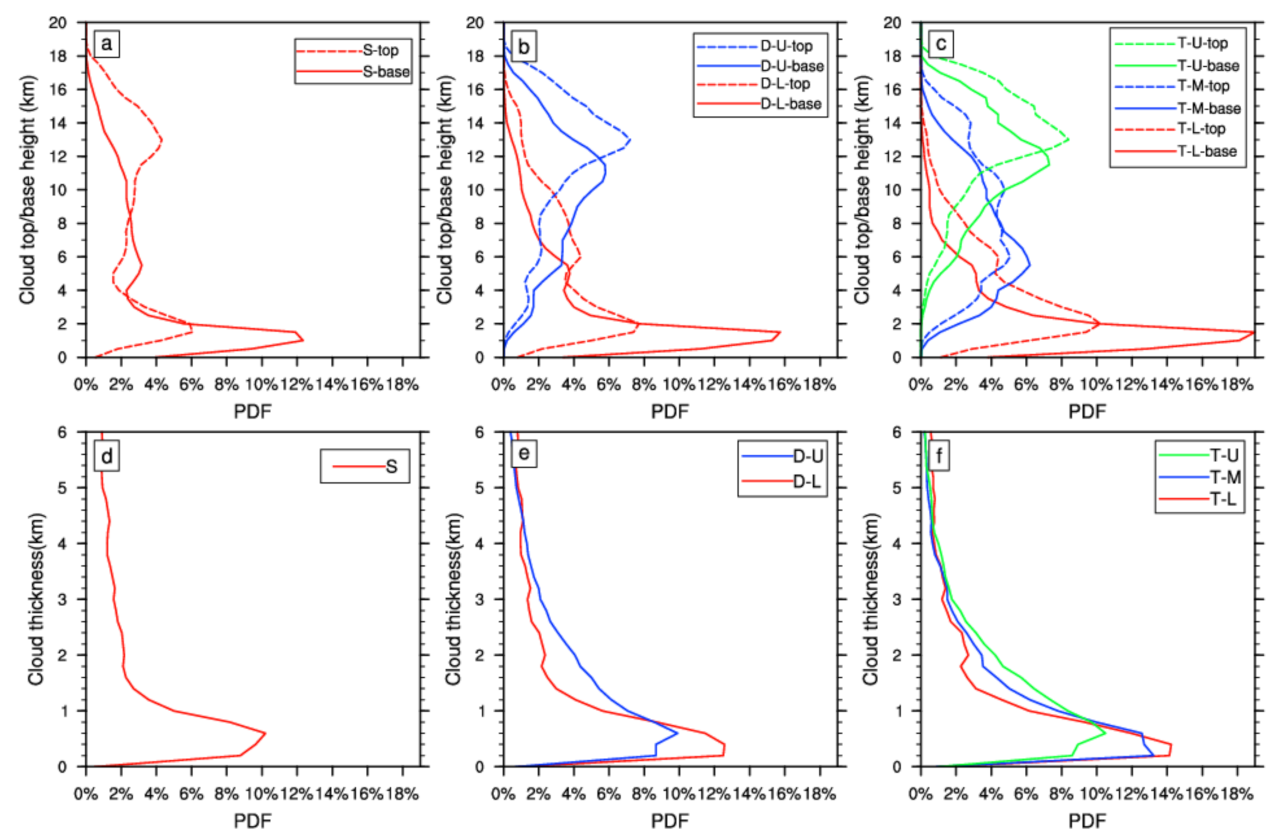
3.2. Cloud Height and Thickness

Cloud-top height (CTH), cloud-base height (CBH) and cloud thickness are important geometric parameters because they usually imply the mechanisms behind the formation of clouds. Because our analysis showed that <3% of the cloud systems had four or more layers, only the results for cloud systems with no more than three layers are reported here due to the distribution of samples. Figure 5 shows the probability distribution functions (PDFs) of CTH, CBH, and cloud thickness for these three kinds of cloud systems.
The CBH of single-layer clouds shows a single-peak distribution with a maximum frequency below 2 km, whereas the CTH has two focal crests at about 2 and 13 km (Figure 5a). This shows that single-layer clouds tend to form at lower levels, but extend to both lower and higher altitudes, indicating two primary single-layer modes: shallow and deep clouds. For multi-layer systems (Figure 5b,c), the CTH and CBH distribution patterns of the cloud layers are unimodal. The lower cloud layers in the double- and triple-layer systems have similar shapes. The CBHs of these two types of layers mainly occur below 2 km and their CTHs are mostly around 2–3 km. By contrast, the peaks of CBH and CTH for the upper layer in the double-layer systems are observed at about 11 and 13 km, much higher than the lower layer (Figure 5b). By comparison, the upper (middle) layers in triple-layer cloud systems are inclined to be elevated (depressed). Namely, the average CBH (CTH) values of the upper layer in double-layer systems are 9.6 (11.4) km, whereas the average CBH (CTH) values of the middle and upper layers in triple-layer systems are 7.3 (8.6) km and 11.3 (12.8) km, respectively.
The results for the distribution of cloud layer thickness (Figure 5d–f), which is derived from the difference between the CTH and CBH, show that all the different kinds of layer show a pronounced unimodal pattern, with a distinct maximum near 0.5 km. The PDFs drop sharply with the occurrence of geometrically thicker clouds and more than half of the clouds are <1 km thick. In general, the thicknesses of layers in certain cloud systems are similar, but, when considering the layers involved in different cloud systems, the cloud thickness usually shifts to smaller values for systems with more layers. Single-layer clouds have an average thickness of 3.4 km, the largest value among the three systems, followed by a mean value of 2.1 km for double-layer clouds. Triple-layer clouds have the smallest average thickness of about 1.5 km.

3.3. Comparison of Single-Layer Precipitating and Non-Precipitating Clouds

In scenarios with multiple cloud layers, it is difficult to determine which layer produces precipitation because the datasets used in this study only provide precipitation identification at the surface. We therefore performed the analyses with single-layer clouds, which clearly demonstrate the differences between precipitating and non-precipitating cloud layers and reveal the characteristics necessary for precipitation.

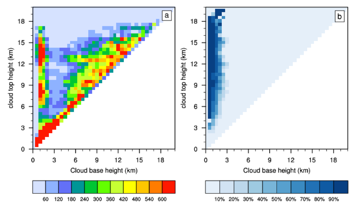
3.3.1. Macrophysical Properties

The number of samples and probability of precipitation (POP) in two-dimensional parameter space are presented for single-layer clouds to recognize the potential correlation between precipitation and cloud geometric parameters. The CBH and CTH groups show a noticeable mode along the major diagonal (Figure 6a), suggesting frequent appearances of geometrically thin clouds at various altitudes. The distribution of single-layer clouds is also concentrated in the left-hand area with CBH < 2 km and CTH 7–15 km (Figure 6a). This indicates the prevalence of thick layers extending from the near surface and associated with deep convection. There are considerable occurrences of higher clouds with a primary mode at a CBH of 7–14 km and a CTH of 8–15 km (Figure 6a), which is partly contributed by anvil and cirrus clouds detrained from deep convection systems. The POP is calculated as the number of precipitating pixels divided by the total number of cloud pixels at given intervals of CBH and CTH (Figure 6b). Samples with a high POP are relatively thick clouds located in the off-diagonal area, as suggested by the mode at a CBH of <3 km and a CTH of 4–18 km. A sufficient vertical extent of cloud is necessary for precipitation [52], however, compared with clouds with a low CBH, clouds with a high CBH are less likely to precipitate even though their thicknesses are the same. The POP shifts from >90% to <30% as the CBH increases to nearly 3 km. POPs > 80% usually coincide with CBHs lower than 1.5 km. In summary, warm season precipitation over the YHRV tends to occur in vigorously developed clouds with low bases and high tops.

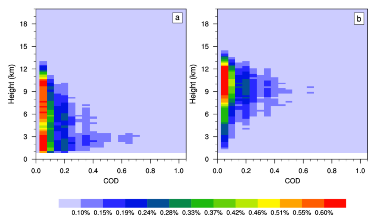
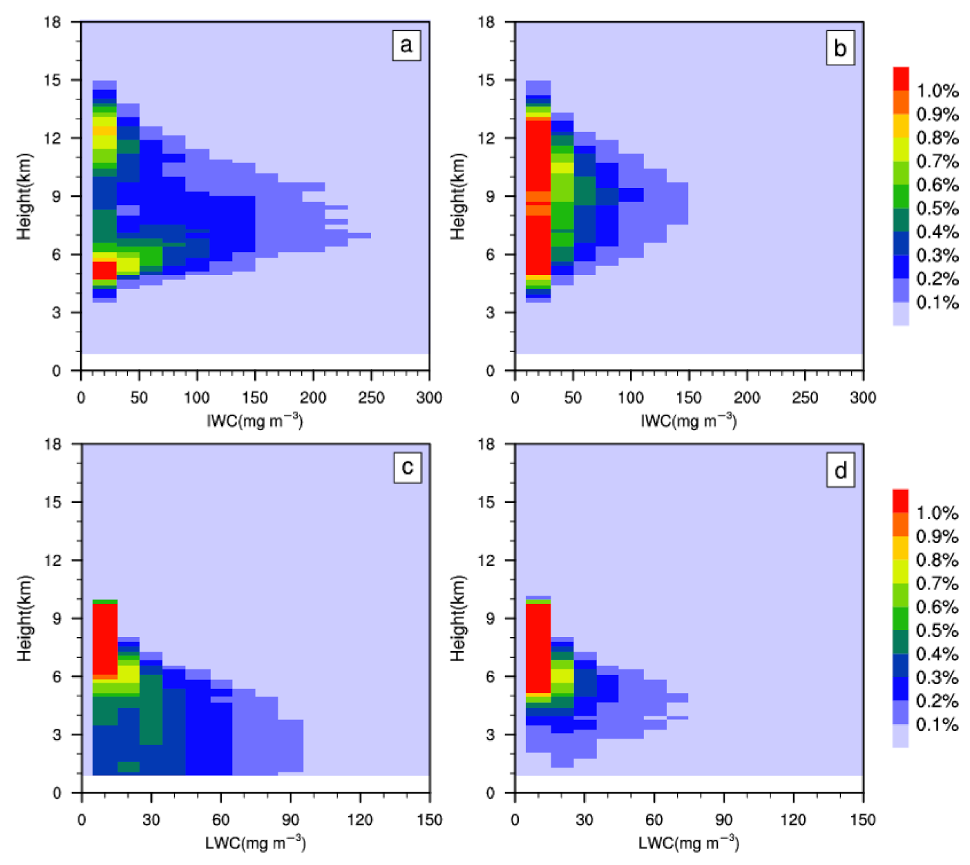
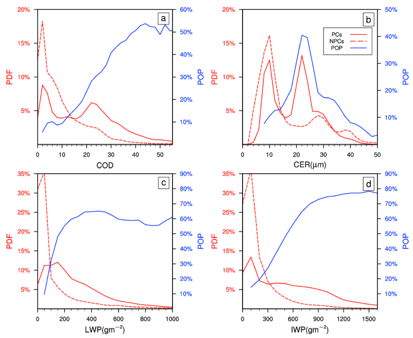
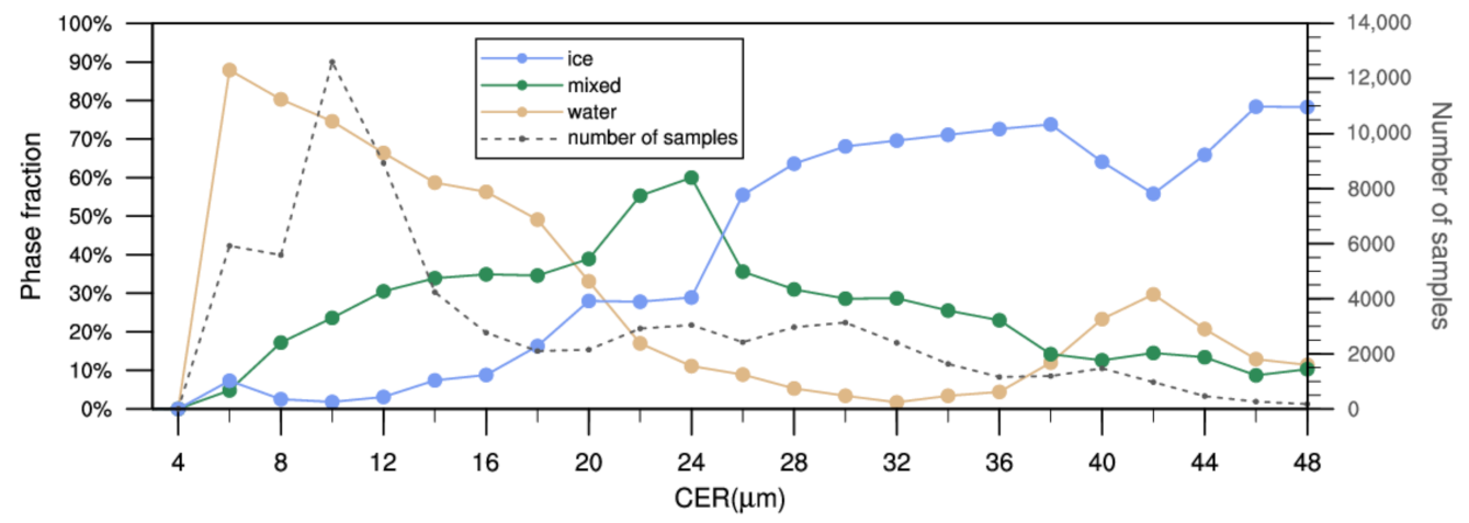
3.3.2. Microphysical Properties

A knowledge of the vertical structure of the microphysical properties has a fundamental role in improving our understanding of the microphysical mechanisms operating in clouds, as well as the simulation and prediction of numerical models. To explore the differences between PCs and NPCs, we calculated the NCFADs for the COD, LWC, and IWC (Figure 7 and Figure 8).
Figure 7 uses vertical slicing of the optical depth. The layered COD is in the range 0.1–0.4 and is <0.1 for both PCs and NPCs throughout the entire column. However, there are some differences. For PCs, the NCFAD distribution shows a trianglular shape, with large CODs at altitudes below 7 km, whereas large CODs of NPCs generally occur at heights of 6–12 km, showing the opposite pattern.
Figure 8 shows the NCFADs of the IWC and LWC to understand the differences in hydrometeor contents. The IWC is broadly found at heights above 5 km, whereas the LWC is mainly distributed at heights below 9 km. One notable feature of PCs is the presence of two IWC peaks (Figure 8a), one at 5–7 km and the other at 10–14 km. The higher peak of the IWC may imply the presence of deep convection. When compared with the values of the IWC for NPCs, PCs are characterized by a larger IWC, which can exceed 150 mg m−3. There is a greater proportion of samples with an IWC < 50 mg m−3 for NPCs (Figure 8b), suggesting a weaker updraft of NPCs according to Heymsfield et al. [53], who showed that the IWC increases with increasing vertical velocity. Similar structures of the LWC are observed for PCs and NPCs at heights above 6 km, where the LWC of each bin is usually <20 mg m−3. Below this level, the LWC of PCs tends to be more spread out and presents higher frequencies at lower altitudes than the LWC of NPCs (Figure 8c,d).
We also examined the statistical characteristics of the vertically integrated properties of clouds. Figure 9 shows PDFs of the COD, CER, LWP, and IWP for PCs and NPCs. The COD (Figure 9a) has a wider range of values for PCs, varying from 0 to >50. The CODs for PCs and NPCs show one and two focal peaks, respectively. The maximum frequency center of NPCs is in the range 0–5, whereas the peak frequencies of PCs are located at values of 3 and 22. These two kinds of cloud are well separated around a COD of about 20; the clouds with a COD < 20 are mostly NPCs, whereas those with a larger COD have a relatively high probability of being PCs. Given the nearly unimodal form of each distribution, the patterns of the LWP and IWP are similar (Figure 9c,d), and are highly centralized for the NPCs and more evenly distributed for the PCs. Although the LWP for PCs has a similar width to that of NPCs, the NPCs have larger proportion of smaller LWPs and a smaller proportion of larger LWPs than the PCs.
Similarly, the occurrence of high IWPs increases notably in PCs compared with NPCs. The IWP of PCs ranges up >1500 g m−2, whereas there is a narrower spread for NPCs, generally <900 g m−2. By contrast, the PDFs of the CER (Figure 9b) for PCs and NPCs, which display multi-peaked structures for both types of clouds, largely overlap with a similar range of 4–45 μm. There is almost no clear boundary in the CER to separate PCs from NPCs, except one dominant peak in the PCs at about 22 μm. With regard to the POP, the trends of the COD, LWP, and IWP are similar—that is, they all increase at first and then remain relatively stable. There is a low POP when the COD/LWP/IWP is small; the POP then increases monotonically until the COD/LWP/IWP increases to about 40/250 g m−2/900 g m−2, reaching a peak of about 50%/60%/75%. These results are consistent with the earlier concept model that PCs are typically associated with sufficient vertical extent and water, with ice particles in the upper part [52,54,55]. The value of 250 g m−2 for the LWP is the threshold recommended by the International Satellite Cloud Climatology Project to screen out PCs. However, the POP of CER has one dominant mode near 22 μm. The POP changes from an increasing to a decreasing trend as the CER increases continuously, in contrast with our perception that large particles fall more easily against updrafts.
Given that the frequency of occurrence of precipitation is related to the thermodynamic phase of clouds [56], and that ice crystals are generally larger than liquid droplets [32], the specific trend of the POP may be attributed to the transition of the cloud phase associated with the increase in the CER. Figure 10 shows the dependence of the cloud phase fraction on the CER, which is defined as the ratio of the number of columns with a specific phase to the total number of cloud columns in a given CER interval. The contribution of water, mixed, and ice clouds changes with the CER. Water clouds, reaching up to >50%, are the dominant form when the CER is <20 μm. There is a dramatic decrease in the fraction of water clouds with increasing CER. Mixed clouds show a relatively stable fraction, but contribute > 60% between 20 and 24 μm, which coincides with the peak POP in Figure 9b. The distribution of ice clouds is the opposite of the distribution of water clouds. Ice clouds hardly occur when the CER is in the range 4–18 mm, but they are often seen when the CER increases further. Overall, these features clearly show the transition of water clouds to mixed clouds and then ice clouds with increasing CER. Based on the statistical results for the POP of clouds with different phases, ice clouds hardly precipitate regardless of the value of CER. We therefore interpret the decreasing trend of POP in Figure 9b as a result of two factors: (1) ice clouds predominate when the CER is >26 μm; and (2) POP is significantly reduced in the ice cloud of YHRV.

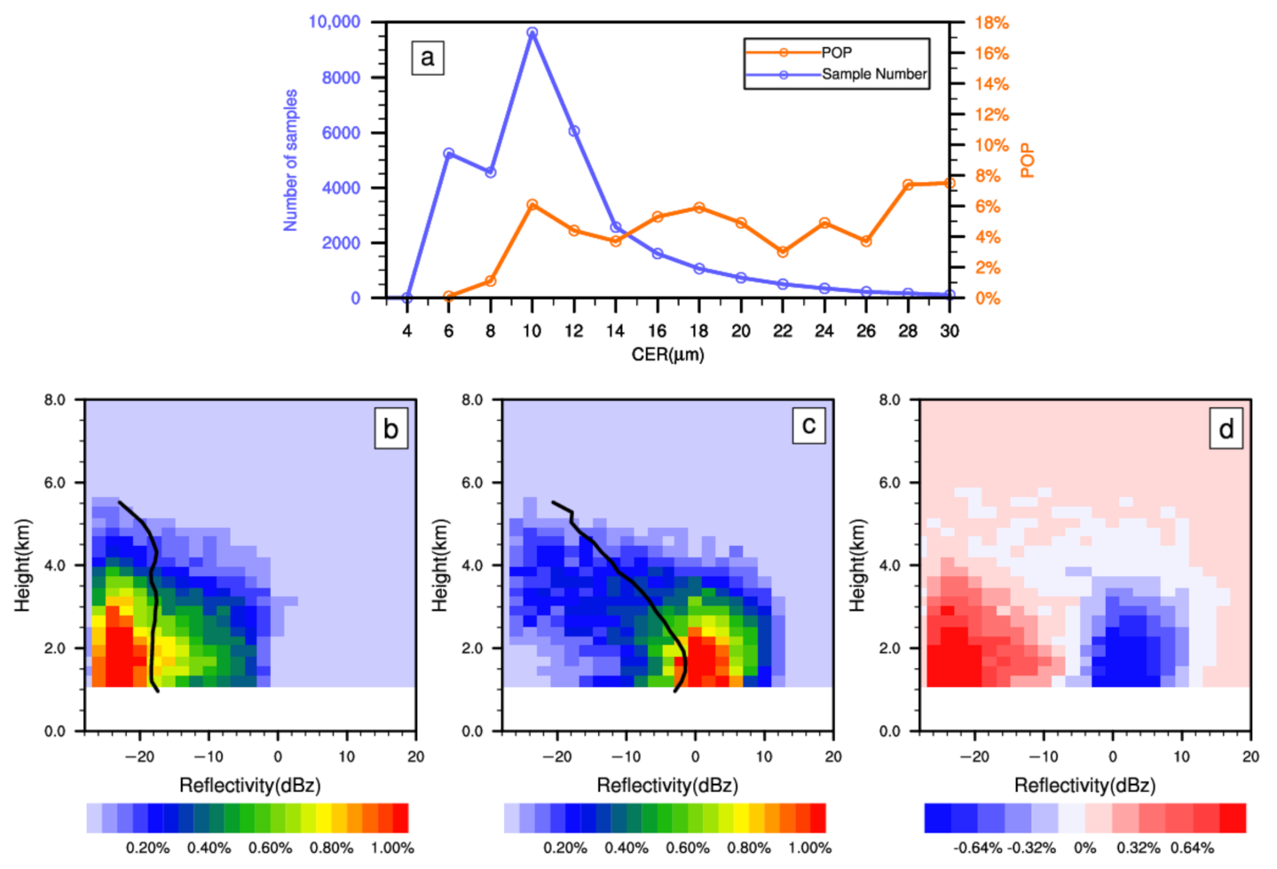
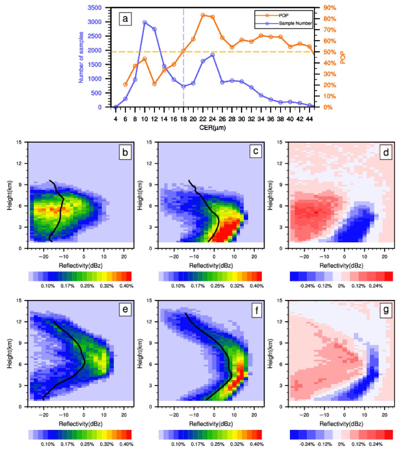
3.3.3. NCFADs of Radar Reflectivity

Our results show that precipitation is produced by water clouds and mixed-phase clouds. We therefore placed single-layer clouds into different categories according to the cloud phase to give a better understanding of precipitation. Figure 11 and Figure 12 show the microphysical differences between PCs and NPCs of water clouds and mixed-phase clouds, respectively.
Figure 11a shows that sample size of single-layer water clouds varies with the CER. Clouds are mainly found in the range of 4–30 μm and reach a peak size at 10 μm. The POP for all single-layer clouds has a unimodal pattern (Figure 10b), but the POP in Figure 11a shows relatively stable trend as the CER increases. In general, the POP of water clouds is <10%, indicative of the scarcity of precipitation from water clouds over the YHRV. We compared the NCFADs of reflectivity for the precipitating and non-precipitating water clouds. Figure 11b,c show that water clouds mainly occurred at altitudes < 6 km. For the NPCs, the maximum frequencies of reflectivity were broadly distributed below −20 dBZ and the maximum reflectivities at different heights were almost all <0 dBZ. Given that the radar reflectivity is proportional to the sixth power of the particle size, it can be regarded as a proxy of the size. The black solid line in Figure 11b, the profile of the mean reflectivity for NPCs, indicates that the radius of the hydrometeors is small because it remains around −18 dBZ between 1 and 5 km. However, the profile of PCs showed a steep gradient (Figure 11c), reflecting a clear downward growth of droplets by collision–coalescence processes. The highest frequencies of PCs were mainly found over the region with reflectivities ranging from −5 to 10 dBZ, which is assigned to drizzle and light rain modes [57]. Apart from the distinct slopes of these profiles, a high radar reflectivity is much more common for PCs (Figure 11d).
Compared with water clouds, mixed-phase clouds have a wider range of CER (Figure 12a). The CER shows a bimodal pattern for mixed-phase single-layer clouds, with two clear peak frequencies at 10 and 24 μm. The POP changes significantly with variation in the CER. As the CER increases, the POP gradually increases and reaches a peak of >80% at CERs between 22 and 24 μm. The POP then fluctuates slightly with further increases in the CER. The POP of mixed-phase clouds is much larger than that of water clouds, indicating the dominant contribution of precipitation from mixed-phase clouds. When a POP = 50% is taken as the critical value, mixed-phase clouds can be subdivided into two separate categories. The POP in the first category is usually <40% and the corresponding CER ranges from 4 to 18 μm. In the second category, in which the CER is >18 μm, the POP is >60%.
The key differences in the POP between the two mixed-phase cloud categories are associated with differences in the CER, which probably result from different cloud microphysical mechanisms [58]. Although both PCs and NPCs can reach an altitude of nearly 9 km in the first category (CER < 18 μm), they show notable differences. NPCs have reflectivities over a broad range above 4 km (Figure 12b), indicating the dispersion of particle sizes. The maximum frequency with reflectivities of −28 to −10 dBZ is mainly located at altitudes of 5–6 km. By contrast, PCs show a peak frequency at altitudes < 5 km, with reflectivities ranging from 0 to 10 dBZ (Figure 12c). Although the mean reflectivity changes slightly with height for NPCs, the profile of PCs tilts toward higher reflectivities with decreasing height to 4 km and then decrease gradually thereafter. Compared with the first category, the reflectivities of the category with CER > 18 μm are shifted to larger values for both NPCs and PCs, showing a distinct peak frequency around 10–15 dBZ.
An arc-like shape is observed for the NCFAD of PCs within the second category (Figure 12f). It resembles the structure in Figure 12c, but extends further along the vertical direction. The radar reflectivities are weak at high altitudes (Figure 12f), but generally increase as the height decreases above 6 km, suggesting the growth of ice particles due to the microphysical processes such as riming and aggregation [59]. High reflectivity dominates in middle layer, and the peak values are centered at about 4.5 km, indicating the location of the melting layer also known as the bright band. This sudden enhancement in reflectivity is probably associated with variations in the dielectric constant and fall velocities of particles as they pass through the melting layer [60]. Because the sample size of PCs in the second category is larger as a result of the higher POP, the vertical structure with the bright band indicates the dominant role of stratiform precipitation in the YHRV, which is consistent with the results from Yang et al. [35]. Below the melting layer, the reflectivity generally decreases downward, which can be attributed to the collapse of melting hydrometeors and the attenuation of signals through optically thick cloud systems [27,61,62]. The NPCs tend to have weaker reflectivities throughout the entire column. NPCs are broadly present at altitudes of 4–9 km and the peak occurrence frequencies are mainly around 0–15 dBZ (Figure 12e). Below 4 km, the reflectivities decrease sharply to less than −20 dBZ near the surface, indicative of strong evaporation and break-up of droplets falling out of clouds. Reflectivities exceeding 10 dBZ above 4 km are associated with the remaining hydrometeors suspended in clouds or falling as drops before reaching the surface [31].

4. Discussions

Ideally, it is meaningful to quantitatively assess the contribution of each precipitating category to surface precipitation, as well as the relationship between surface rain rates and cloud properties. However, due to the limitations of CPR products, precipitation intensity of each pixel is not available in our study area. Specifically, the algorithm of CPR makes use of the radar reflectivity near the surface of the earth and an estimate of path integrated attenuation determined from the surface reflection characteristics to determine precipitation incidence and intensity [44]. Since CPR echoes at the lowest two or three bins are contaminated by strong surface clutter, there is an almost blind zone from surface to nearly 1 km [47,63]. Precipitation intensity is only reported over open-water surfaces. Therefore, the rainfall datasets from meteorological stations covering YHRV are used for further study. Each CPR pixel is matched with an hourly rainfall of the closest time using the linear nearest distance method.
According to the approaches of Lu et al. [64], area fraction (AF) is used to quantitatively evaluate the observed sample proportion of each precipitation category, and contribution fraction (CF) is calculated to show the rainfall contribution from each category to total rainfall in the YHRV. In detail, a larger AF represents for larger occurrence frequency, and a larger CF indicates a larger contribution to total rainfall. Statistical results show that the contribution of each precipitating category are different, the AF (CF) is 6% (2%) for water PCs, 30.8% (19.5%) for mixed PCs with CER < 18 μm, and 63.2% (78.5%) for mixed PCs with CER ≥ 18 μm, respectively. In other words, the AF for water PCs is 6%, while the sample proportion of mixed PCs is 94%. The corresponding contribution to total precipitation of mixed PCs can reach 98%, while the CF for water PCs is only 2%.
The relationships between surface rain rates and cloud properties are investigated in Figure 13. Generally, surface rain rate of PCs increases from 1 mm/h gradually to nearly 4 mm/h with the increment of CER at first, and then shows a decreasing trend as CER increases further (Figure 13a). The heaviest precipitation falls in the range of 20–30 μm, consistent with the result presented by Cattani et al. [65]. However, no clear relationship is found between COD and precipitation intensity of PCs (Figure 13b), rain rates stay relatively stable with the COD spanning from 10 to 40, which needs to be further explored in future work. In Figure 13c, when LWP is low, rain rate increases as LWP increases. By contrast, a notable decrease in rain rate is shown for LWP > 500 g m−2. One possible reason could be that the descending trend is contributed by dissipating convections, the LWP of the dissipating stage clouds is larger than that in developing stage, whereas it is opposite for precipitation intensity [66]. In Figure 13d, rain rate of PCs obviously increases as IWP increases, associated with stronger updrafts and vigorous convection corresponding to larger IWP. In summary, we give a preliminary assessment of the impact of cloud properties on precipitation intensity by combining observations from satellites and ground-based stations. The precipitation mechanism and its relationship with cloud characteristics is fairly complicated and dynamic activity, the completion of an improved analysis requires more simultaneous in situ measurements as well as the validation from numerical models, which is beyond the scope of the present study.
It is also important to clarify some limitations of this study. Although the CloudSat product is by far make remarkable progress in observing cloud and precipitation, the sparse temporal sampling of CPR measurements may result in biases in our results due to its sun-synchronous orbit with only two overpasses at about 13:30 local time during the daytime and 01:30 local time during nighttime. However, according to Battaglia et al. [67], CloudSat CPR remains the only existing (until 2020) spaceborne radar with a frequency of W-band, which is the preferred cloud-sensing frequency with sufficient sensitivity to detect most hydrologically important clouds. There is currently no other appropriate instrument to provide supplementary observations of cloud internal structure in the study area, which can enable us to conduct a more comprehensive analysis. Additionally, as indicated by Liu et al. [68], the occurrence of precipitation and cloud averaged from both the day and night CloudSat data are close to the mean results derived from 9-year full day samples of Tropical Rainfall Measuring Mission (TRMM). Therefore, both day and night-time measurements are adopted in this study to minimize biases caused by low sampling as much as possible.
We use the products from 2007 to 2010 for analysis since the longer-term CPR data used in this study is not available. CloudSat was launched in 2006 to join the A-train constellation, but temporarily left A-train in 2011 as a result of a spacecraft battery failure and then returned to the A-train but behind Calipso on 15 May 2012. After that, the CPR is operated in the so-called “Daylight Only” mode. Therefore, the product during 2007–2010 would be continuous observations with good consistency in time and space with A-train. We reviewed related works from the literature when conducting this study. To our knowledge, there are many studies regulating the data interval within 2007 to 2010 [2,41,69,70]. In addition, large-scale processes do have impacts on clouds and precipitation. According to previous studies [64,71], the western North Pacific subtropical high (WNPSH) is the major atmospheric system controlling the East Asia summer monsoon behaviors. They showed that WNPSH has significant impacts on summer precipitation over Eastern China. Specifically, Zhang et al. [71] investigated temporal changes of WNPSH and the summer precipitation of eastern China during 1961–2010. They found that the correlation coefficient between the areal average summer precipitation and the WNPSH index is −0.46, significant at the 99% confidence level. From 2007 to 2010, both the WNPSH index and standardized regional precipitation anomaly are inside the range of ±1 standard deviation from the mean without significant abnormalities. Therefore, it is suggested that the large-scale circulation and precipitation during our study period are close to the annual average state and our conclusions are potentially representative.

5. Conclusions

By using five standard CloudSat products, which synthesize observations from CPR, CALIOP, and MODIS, we have illustrated cloud characteristics regarding the occurrence frequency, vertical arrangements and distinctions between NPCs and PCs over the YHRV during the warm season. The notable results can be summarized as follows:
Clouds are most likely to appear at altitudes of 7 km, with a cloud fraction > 21% over the YHRV during the warm season. Single-layer clouds are the most fundamental form, making up nearly 56% of the total frequency of clouds, followed by double-layer clouds with a frequency of 31%. Cloud systems with three or four layers are rare. Single- and multi-layer cloud systems have distinct geometrical features. Single-layer clouds are the dominant form of PCs.
The macrophysical properties show that warm season precipitation tends to be generated from clouds with a lower CBH and higher CTH; clouds with a low POP mainly correspond to clouds with a smaller geometric thickness. There is a clear difference between NPCs and PCs with regard to the internal structure of the microphysical properties, reflecting inherent difference in the dynamic and microphysical processes of clouds, such as updraft strength or the coalescence/break-up of water droplets. In addition to confirming several known features of PCs—such as sufficient vertical extent, abundant water, and the existence of ice particles—we quantitatively showed that the POP increases to 50%/60%/75% as the COD/LWP/IWP increases. The POP shows an increasing trend with increasing cloud effective radius (CER) when the CER was <22 μm, but a decreasing trend when the CER was >22 μm, which is in contrast with our perception that large particles fall more easily against updrafts. However, this can be attributed to the transition of the cloud phase from a water cloud to an ice cloud.
Clouds were categorized into two groups depending on their phase. The most striking feature was the scarcity of precipitation from water clouds, with a maximum POP of <10%. Only a few samples had a CER > 14 μm, which is regarded as the initial threshold for warm rain [72,73]. Since it is difficult for water cloud droplets to grow to the precipitating size, the phenomenon is probably driven by the relatively heavy aerosol loadings in this region [35]. According to Fu et al. [74], the frequency and intensity of summer precipitations in YHRV are associated with the aerosol concentration in the lower atmosphere. Given that the location of warm clouds is relatively lower, it is easier for aerosols to enter in, and then reduce particle sizes to suppress warm-rain processes through aerosol indirect effects [75,76]. Mixed clouds are more likely to precipitate over the YHRV than warm clouds, indicating their significant contribution to precipitation. More specifically, PCs are usually associated with the prevalence of reflectivities > 0 dBZ, as well as the significant downward growth of particles, potentially a result of processes such as aggregation or coalescence. NPCs, by contrast, are typically characterized by weaker reflectivity throughout the entire column with less variation, or strong evaporation below large reflectivities concentrated above 5 km.
The use of thresholds (CER = 18 μm) to distinguish two mixed-cloud categories yielded some differences. The vertical extent of the second category develops at higher altitudes (>12 km). Given the higher POP of the second category, these results imply that vigorous ice-phase microphysical processes are important for the occurrence of surface precipitation over the YHRV in the warm season, further confirming the role of sufficient vertical development for droplet growth.
This study is a preliminary comparison of PCs and NPCs over the YHRV and provides researchers with benchmarks to evaluate the treatability of clouds with weather modification technologies. There is an increasing socioeconomic demand for monitoring and managing atmospheric water to protect the regional ecology, including resolving droughts and preventing forest fire. Precipitation enhancement experiments should remain at the forefront of current research. Specific studies are required to explore the underlying physical regimes that induce the low probability of warm cloud precipitation, which will help to give a complete characterization of seedable clouds and inform the scientific conduction of weather modification activities.

Author Contributions

Y.Y. (Yuanjian Yang) proposed the study. X.Z. collected data and performed the analysis. X.Z. and Y.Y. (Yuanjian Yang) wrote the manuscript. Y.Y. (Ye Yuan), Y.C. and J.G. helped with the data preparation and participated in discussions of the results. All authors have read and agreed to the published version of the manuscript.

Funding

This work was Supported by the National Key Research and Development Program of China (2019YFC1510303) and National Natural Science Foundation of China (42175098).

Institutional Review Board Statement

Not applicable.

Informed Consent Statement

Not applicable.

Data Availability Statement

The satellite data used in this study were got from the CloudSat website http://www.CloudSat.cira.colostate.edu, accessed on 26 October 2021. The precipitation product is available online from http://data.cma.cn, accessed on 26 October 2021.

Acknowledgments

We would like to thank the NASA CloudSat team for sharing CPR product data in the CloudSat Data Processing Center. We are also grateful to the editors’ and referees’ efforts in improving the manuscript.

Conflicts of Interest

The authors declare no conflict of interest.

References

  1. Hartmann, D.L.; Ockert-Bell, M.E.; Michelsen, M.L. The Effect of Cloud Type on Earth’s Energy Balance: Global Analysis. J. Clim. 1992, 5, 1281–1304. [Google Scholar] [CrossRef] [Green Version]
  2. Eric, E.; Wandjie, B.B.; Lenouo, A.; Monkam, D.; Manatsa, D. African summer monsoon active and break spells cloud properties: Insight from CloudSat-CALIPSO. Atmos. Res. 2020, 237, 104842. [Google Scholar] [CrossRef]
  3. Sassen, K.; Wang, Z. The clouds of the middle troposphere: Composition, radiative impact, and global distribution. Surv. Geophys. 2011, 33, 677–691. [Google Scholar] [CrossRef]
  4. Turner, D.D.; Vogelmann, A.M.; Austin, R.T.; Barnard, J.C.; Cady-Pereira, K.; Chiu, J.C.; Clough, S.A.; Flynn, C.; Khaiyer, M.M.; Liljegren, J.; et al. Thin liquid water clouds: Their importance and our challenge. Bull. Am. Meteor. Soc. 2007, 88, 177–190. [Google Scholar] [CrossRef]
  5. Liu, D.; Liu, Q.; Liu, G.; Wei, J.; Deng, S.; Fu, Y. Multiple factors explaining the deficiency of cloud profiling radar on detecting oceanic warm clouds. J. Geophys. Res. Atmos. 2018, 123, 8135–8158. [Google Scholar] [CrossRef]
  6. Donovan, D.P.; Klein, B.H.; Henzing, J.S.; De Roode, S.R.; Siebesma, A.P. A depolarisation lidar-based method for the determination of liquid-cloud microphysical properties. Atmos. Meas. Tech. 2015, 8, 237–266. [Google Scholar] [CrossRef] [Green Version]
  7. Gultepe, I.; Isaac, G.A.; Strawbridge, K.B. Variability of cloud microphysical and optical parameters obtained from aircraft and satellite remote sensing measurements during RACE. Int. J. Climatol. 2001, 21, 507–525. [Google Scholar] [CrossRef]
  8. Boucher, O.; Randall, D.; Artaxo, P.; Bretherton, C.; Feingold, G.; Forster, P.; Kerminen, V.; Kondo, Y.; Liao, H.; Lohmann, U.; et al. Clouds and aerosols. In Climate Change 2013: The Physical Science Basis. Contribution of Working Group I to the Fifth Assessment Report of the Intergovernmental Panel on Climate Change; Stocker, T.F., Qin, D., Eds.; Cambridge University Press: New York, NY, USA, 2014; pp. 866–871. [Google Scholar]
  9. Hong, Y.; Liu, G.; Li, J.L. Assessing the radiative effects of global ice clouds based on CloudSat and CALIPSO measurements. J. Clim. 2016, 29, 7651–7674. [Google Scholar] [CrossRef]
  10. Miao, H.; Wang, X.; Liu, Y.; Wu, G. An evaluation of cloud vertical structure in three reanalyses against CloudSat/cloud—aerosol lidar and infrared pathfinder satellite observations. Atmos. Sci. Lett. 2019, 20, e906. [Google Scholar] [CrossRef] [Green Version]
  11. Daloz, A.S.; Nelson, E.; L’Ecuyer, T.; Rapp, A.D.; Sun, L. Assessing the Coupled Influences of Clouds on the Atmospheric Energy and Water Cycles in Reanalyses with A-Train Observations. J. Clim. 2018, 31, 8241–8264. [Google Scholar] [CrossRef]
  12. Sun, G.; Li, Y.; Li, S. The differences in cloud vertical structures between active and break spells of the East Asian summer monsoon based on CloudSat data. Atmos. Res. 2019, 224, 157–167. [Google Scholar] [CrossRef]
  13. Hang, Y.; L’Ecuyer, T.S.; Henderson, D.S.; Matus, A.V.; Wang, Z. Reassessing the effect of cloud type on Earth’s energy balance in the age of active spaceborne observations. Part II: Atmospheric heating. J. Clim. 2019, 32, 6219–6236. [Google Scholar] [CrossRef]
  14. Schumacher, C.; Zhang, M.H.; Ciesielski, P.E. Heating structures of the TRMM field campaigns. J. Atmos. Sci. 2007, 64, 2593–2610. [Google Scholar] [CrossRef]
  15. Lau, K.M.; Wu, H.T. Warm rain processes over tropical oceans and climate implications. Geophy. Res. Lett. 2004, 30. [Google Scholar] [CrossRef]
  16. Tao, W.K.; Takayabu, Y.N.; Lang, S.; Shige, S.; Olson, W.; Hou, A.; Skofronick, J.G.; Jiang, X.; Zhang, C.; Lau, W.; et al. TRMM latent heating retrieval: Applications and comparisons with field campaigns and large-scale analyses. Meteorol. Monogr. 2016, 56, 2.1–2.34. [Google Scholar] [CrossRef]
  17. Nelson, E.L.; L’Ecuyer, T.S. Global character of latent heat release in oceanic warm rain systems. J. Geophys. Res. Atmos. 2018, 123, 4797–4817. [Google Scholar] [CrossRef]
  18. Jakob, C.; Klein, S.A. The role of vertically varying cloud fraction in the parametrization of microphysical processes in the ECMWF model. Q. J. R. Meteorol. Soc. 1999, 125, 941–965. [Google Scholar] [CrossRef]
  19. Yan, Y.F.; Wang, X.C.; Liu, Y.M. Cloud vertical structures associated with precipitation magnitudes over the Tibetan Plateau and its neighboring regions. Atmos. Ocean. Sci. Lett. 2018, 11, 44–53. [Google Scholar] [CrossRef] [Green Version]
  20. Klein, S.A.; Zhang, Y.; Zelinka, M.D.; Pincus, R.; Boyle, J.; Gleckler, P.J. Are climate model simulations of clouds improving? An evaluation using the ISCCP simulator. J. Geophys. Res. Atmos. 2013, 118, 1329–1342. [Google Scholar] [CrossRef]
  21. Cesana, G.; Del Genio, A.D.; Chepfer, H. The cumulus and stratocumulus cloudsat-calipso dataset (casccad). Earth Syst. Sci. Data 2019, 11, 1745–1764. [Google Scholar] [CrossRef] [Green Version]
  22. Hong, Y.; Di Girolamo, L. Cloud phase characteristics over Southeast Asia from A-Train satellite observations. Atmos. Chem. Phys. 2020, 20, 8267–8291. [Google Scholar] [CrossRef]
  23. Stephens, G.L.; Vane, D.G.; Boain, R.J.; Mace, G.G.; Sassen, K.; Wang, Z.; Illingworth, A.J.; O’connor, E.J.; Rossow, W.B.; Durden, S.L.; et al. The CloudSat mission and the A-Train: A new dimension of space-based observations of clouds and precipitation. Bull. Am. Meteor. Soc. 2002, 83, 1771–1790. [Google Scholar] [CrossRef] [Green Version]
  24. Winker, D.M.; Pelon, J.R.; McCormick, M.P. The CALIPSO mission: Spaceborne lidar for observation of aerosols and clouds. Proc. SPIE Int. Soc. Opt. Eng. 2003, 4893, 1–11. [Google Scholar] [CrossRef] [Green Version]
  25. Stephens, G.L.; Vane, D.G.; Tanelli, S.; Im, E.; Durden, S.; Rokey, M.; Reinke, D.; Partain, P.; Mace, G.G.; Austin, R. CloudSat mission: Performance and early science after the first year of operation. J. Geophys. Res. Atmos. 2008, 113. [Google Scholar] [CrossRef]
  26. Luo, Y.; Zhang, R.; Wang, H. Comparing occurrences and vertical structures of hydrometeors between eastern China and the Indian monsoon region using CloudSat/CALIPSO data. J. Clim. 2009, 22, 1052–1064. [Google Scholar] [CrossRef]
  27. Das, S.K.; Golhait, R.B.; Uma, K.N. Clouds vertical properties over the Northern Hemisphere monsoon regions from CloudSat-CALIPSO measurements. Atmos. Res. 2017, 183, 73–83. [Google Scholar] [CrossRef]
  28. Kukulies, J.; Chen, D.; Wang, M. Temporal and spatial variations of convection and precipitation over the Tibetan Plateau based on recent satellite observations. Part I: Cloud climatology derived from CloudSat and CALIPSO. Int. J. Climatol. 2019, 39, 5396–5412. [Google Scholar] [CrossRef] [Green Version]
  29. Yu, L.; Fu, Y.; Yang, Y.; Pan, X.; Tan, R. Trumpet-shaped topography modulation of the frequency, vertical structures, and water path of cloud systems in the summertime over the southeastern Tibetan Plateau: A perspective of daytime—Nighttime differences. J. Geophys. Res. Atmos. 2020, 125, e2019JD031803. [Google Scholar] [CrossRef]
  30. Fu, Y.; Ma, Y.; Zhong, L.; Yang, Y.; Guo, X.; Wang, C.; Xu, X.; Yang, K.; Xu, X.; Liu, L.; et al. Land-surface processes and summer-cloud-precipitation characteristics in the Tibetan Plateau and their effects on downstream weather: A review and perspective. Natl. Sci. Rev. 2020, 7, 500–515. [Google Scholar] [CrossRef] [PubMed] [Green Version]
  31. Gao, W.; Sui, C.H.; Hu, Z. A study of macrophysical and microphysical properties of warm clouds over the Northern Hemisphere using CloudSat/CALIPSO data. J. Geophys. Res. Atmos. 2014, 119, 3268–3280. [Google Scholar] [CrossRef]
  32. Kikuchi, M.; Suzuki, K. Characterizing vertical particle structure of precipitating cloud system from multiplatform measurements of A-Train constellation. Geophys. Res. Lett. 2019, 46, 1040–1048. [Google Scholar] [CrossRef] [Green Version]
  33. Li, S.; Li, Y.; Sun, G.; Lu, Z. Macro- and Microphysical Characteristics of Precipitating and Non-Precipitating Stratocumulus Clouds over Eastern China. Atmosphere 2018, 9, 237. [Google Scholar] [CrossRef] [Green Version]
  34. Stephens, G.L.; Kummerow, C.D. The remote sensing of clouds and precipitation from space: A review. J. Atmos. Sci. 2007, 64, 3742–3765. [Google Scholar] [CrossRef]
  35. Yang, Y.; Wang, H.; Chen, F.; Zheng, X.; Fu, Y.; Zhou, S. TRMM-Based Optical and Microphysical Features of Precipitating Clouds in Summer Over the Yangtze—Huaihe River Valley, China. Pure Appl. Geophys. 2019, 176, 357–370. [Google Scholar] [CrossRef]
  36. Stein, T.H.M.; Parker, D.J.; Delanoe, J.; Dixon, N.S.; Hogan, R.J.; Knippertz, P.; Maidment, R.I.; Marsham, J.H. The vertical cloud structure of the West African monsoon: A 4 year climatology using CloudSat and CALIPSO. J. Geophys. Res. Space Phys. 2011, 116, D22205. [Google Scholar] [CrossRef] [Green Version]
  37. Marchand, R.; Mace, G. Level 2 GEOPROF Product Process Description and Interface Control Document. Available online: https://www.cloudsat.cira.colostate.edu/cloudsat-static/info/dl/2b-geoprof/2B-GEOPROF_PDICD.P1_R05.rev0__0.pdf (accessed on 26 October 2021).
  38. Ding, Y.; Liu, Q.; Lao, P. Characteristics of Oceanic Warm Cloud Layers within Multilevel Cloud Systems Derived by Satellite Measurements. Atmosphere 2019, 10, 465. [Google Scholar] [CrossRef] [Green Version]
  39. Polonsky, I.N.; Labonnote, L.C.; Cooper, S. Level 2 Cloud Optical Depth Product Process Description and Interface Control Document. Available online: https://www.cloudsat.cira.colostate.edu/cloudsat-static/info/dl/2b-tau/2B-TAU_PDICD.P_R04.20080220.pdf (accessed on 26 October 2021).
  40. Liu, Y.; Shupe, M.D.; Wang, Z.; Mace, G. Cloud vertical distribution from combined surface and space radar-lidar observations at two Arctic atmospheric observatories. Atmos. Chem. Phys. 2017, 17, 5973–5989. [Google Scholar] [CrossRef] [Green Version]
  41. Li, X.; Zheng, X.; Zhang, D.; Zhang, W.; Wang, F.; Deng, Y.; Zhu, W. Clouds over East Asia Observed with Collocated CloudSat and CALIPSO Measurements: Occurrence and Macrophysical Properties. Atmosphere 2018, 9, 168. [Google Scholar] [CrossRef] [Green Version]
  42. Wang, Z. CloudSat 2B-CLDCLASS-LIDAR Product Process Description and Interface Control Document. Available online: https://www.cloudsat.cira.colostate.edu/cloudsat-static/info/dl/2b-cldclass-lidar/2B-CLDCLASS-LIDAR_PDICD.P1_R05.rev0_.pdf (accessed on 26 October 2021).
  43. Leinonen, J. Level 2B CWC-RVOD Product Process Description and Interface Control Document. Available online: https://www.cloudsat.cira.colostate.edu/cloudsat-static/info/dl/2b-cwc-rvod/2B-CWC-RVOD_PDICD.P1_R05.rev0_.pdf (accessed on 26 October 2021).
  44. Haynes, J.M. CloudSat 2C-PRECIP-COLUMN Data Product Process Description and Interface Control Document. Available online: https://www.cloudsat.cira.colostate.edu/cloudsat-static/info/dl/2c-precip-column/2C-PRECIP-COLUMN_PDICD.P1_R05.rev1_.pdf (accessed on 26 October 2021).
  45. Hagihara, Y.; Okamoto, H.; Yoshida, R. Development of a combined CloudSat-CALIPSO cloud mask to show global cloud distribution. J. Geophys. Res. Atmos. 2010, 115. [Google Scholar] [CrossRef] [Green Version]
  46. Marchand, R.; Mace, G.G.; Ackerman, T.; Stephens, G. Hydrometeor detection using CloudSat—An Earth-orbiting 94-GHz cloud radar. J. Geophys. Res. Atmos. 2008, 25, 519–533. [Google Scholar] [CrossRef]
  47. Liu, D.; Liu, Q.; Qi, L.; Fu, Y. Oceanic single-layer warm clouds missed by the cloud profiling radar as inferred from modis and caliop measurements. J. Geophys. Res. Atmos. 2016, 121, 12947–12965. [Google Scholar] [CrossRef]
  48. Yuter, S.E.; Houze, R.A., Jr. Three-dimensional kinematic and microphysical evolution of Florida cumulonimbus. Part III: Vertical mass transport, mass divergence, and synthesis. Mon. Weather Rev. 1995, 123, 1964–1983. [Google Scholar] [CrossRef] [Green Version]
  49. Guo, J.; Liu, H.; Li, Z.; Rosenfeld, D.; Jiang, M.; Xu, W.; Jiang, J.H.; He, J.; Chen, D.; Min, M.; et al. Aerosol-induced changes in the vertical structure of precipitation: A perspective of TRMM precipitation radar. Atmos. Chem. Phys. 2018, 18, 13329–13343. [Google Scholar] [CrossRef] [Green Version]
  50. Luo, J.; Tian, W.; Pu, Z.; Zhang, P.; Shang, L.; Zhang, M.; Hu, J. Characteristics of stratosphere-troposphere exchange during the Meiyu season. J. Geophys. Res. Atmos. 2013, 118, 2058–2072. [Google Scholar] [CrossRef] [Green Version]
  51. Chen, X.; Zhang, F.; Zhao, K. Influence of monsoonal wind speed and moisture content on intensity and diurnal variations of the mei-yu season coastal rainfall over south China. J. Atmos. Sci. 2017, 74, 2835–2856. [Google Scholar] [CrossRef]
  52. Nauss, T.; Kokhanovsky, A.A. Discriminating raining from non-raining clouds at mid-latitudes using multispectral satellite data. Atmos. Chem. Phys. 2006, 6, 5031–5036. [Google Scholar] [CrossRef] [Green Version]
  53. Heymsfield, A.J.; Donner, L.J. A scheme for parameterizing ice-cloud water content in general circulation models. J. Atmos. Sci. 1990, 47, 1865–1877. [Google Scholar] [CrossRef] [Green Version]
  54. Thies, B.; Nauss, T.; Bendix, J. Discriminating raining from non-raining clouds at mid-latitudes using meteosat second generation daytime data. Atmos. Chem. Phys. 2008, 8, 2341–2349. [Google Scholar] [CrossRef] [Green Version]
  55. Chen, F.; Sheng, S.; Bao, Z.; Wen, H.; Hua, L.; Paul, N.J.; Fu, Y. Precipitation clouds delineation scheme in tropical cyclones and its validation using precipitation and cloud parameter datasets from TRMM. J. Appl. Meteorol. Clim. 2018, 57, 821–836. [Google Scholar] [CrossRef]
  56. Mülmenstädt, J.; Sourdeval, O.; Delanoë, J.; Quaas, J. Frequency of occurrence of rain from liquid-, mixed-, and ice-phase clouds derived from A-Train satellite retrievals. Geophys. Res. Lett. 2015, 42, 6502–6509. [Google Scholar] [CrossRef] [Green Version]
  57. Nakajima, T.Y.; Suzuki, K.; Stephens, G.L. Droplet growth in warm water clouds observed by the A-Train. Part II: A multisensor view. J. Atmos. Sci. 2010, 67, 1897–1907. [Google Scholar] [CrossRef]
  58. Kumjian, M.R.; Prat, O.P. The impact of raindrop collisional processes on the polarimetric radar variables. J. Atmos. Sci. 2014, 71, 3052–3067. [Google Scholar] [CrossRef]
  59. Houze, R.A., Jr. Cloud Dynamics, 2nd ed.; Academic Press: Cambridge, MA, USA, 2014; p. 58. [Google Scholar]
  60. Mubara, K.; Dawood, A.; Al Dosary, A. Global mapping of height of bright band. In Proceedings of the 2007 9th International Symposium on Signal Processing and Its Applications, Sharjah, United Arab Emirates, 12–15 February 2007. [Google Scholar] [CrossRef]
  61. Matrosov, S.Y. Potential for attenuation-based estimations of rainfall rate from CloudSat. Geophys. Res. Lett. 2007, 34, L05817. [Google Scholar] [CrossRef] [Green Version]
  62. Christensen, M.W.; Stephens, G.L.; Lebsock, M.D. Exposing biases in retrieved low cloud properties from CloudSat: A guide for evaluating observations and climate data. J. Geophys. Res. Atmos. 2013, 118, 12120–12131. [Google Scholar] [CrossRef]
  63. Mace, G.G.; Marchand, R.; Zhang, Q.; Stephens, G. Global hydrometeor occurrence as observed by CloudSat: Initial observations from summer 2006. Geophys. Res. Lett. 2007, 34, L09808. [Google Scholar] [CrossRef] [Green Version]
  64. Lu, D.; Yang, Y.; Fu, Y. Interannual variability of summer monsoon convective and stratiform precipitation in East Asia during 1998–2013. Int. J. Climatol. 2016, 36, 3507–3520. [Google Scholar] [CrossRef]
  65. Cattani, E.; Torricella, F.; Laviola, S.; Levizzani, V. On the statistical relationship between cloud optical and microphysical characteristics and rainfall intensity for convective storms over the Mediterranean. Nat. Hazards Earth Syst. Sci. 2009, 9, 2135–2142. [Google Scholar] [CrossRef] [Green Version]
  66. Zhang, A.; Fu, Y. Life cycle effects on the vertical structure of precipitation in East China measured by Himawari-8 and GPM DPR. Mon. Weather Rev. 2018, 146, 2183–2199. [Google Scholar] [CrossRef]
  67. Battaglia, A.; Kollias, P.; Dhillon, R.; Roy, R.; Tanelli, S.; Lamer, K.; Grecu, M.; Lebsock, M.; Watters, D.; Mroz, K.; et al. Spaceborne cloud and precipitation radars: Status, challenges, and ways forward. Rev. Geophys. 2020, 58, e2019RG000686. [Google Scholar] [CrossRef] [PubMed]
  68. Liu, C.; Zipser, E.J.; Mace, G.G.; Benson, S. Implications of the differences between daytime and nighttime CloudSat observations over the tropics. J. Geophys. Res. Atmos. 2008, 113, D00A04. [Google Scholar] [CrossRef] [Green Version]
  69. Peng, J.; Zhang, H.; Li, Z. Temporal and spatial variations of global deep cloud systems based on CloudSat and CALIPSO satellite observations. Adv. Atmos. Sci. 2014, 31, 593–603. [Google Scholar] [CrossRef]
  70. Oreopoulos, L.; Cho, N.; Lee, D. New insights about cloud vertical structure from CloudSat and CALIPSO observations. J. Geophys. Res. Atmos. 2017, 122, 9280–9300. [Google Scholar] [CrossRef]
  71. Zhang, Q.; Zheng, Y.; Singh, V.P.; Luo, M.; Xie, Z. Summer extreme precipitation in eastern China: Mechanisms and impacts. J. Geophys. Res. Atmos. 2017, 122, 2766–2778. [Google Scholar] [CrossRef]
  72. Rosenfeld, D.; Wang, H.; Rasch, P.J. The roles of cloud drop effective radius and LWP in determining rain properties in marine stratocumulus. Geophys. Res. Lett. 2012, 39, L13801. [Google Scholar] [CrossRef]
  73. Zhu, Y.; Rosenfeld, D.; Yu, X.; Li, Z. Separating aerosol microphysical effects and satellite measurement artifacts of the relationships between warm rain onset height and aerosol optical depth. J. Geophys. Res. Atmos. 2015, 120, 7726–7736. [Google Scholar] [CrossRef]
  74. Fu, Y.; Pan, X.; Yang, Y.; Chen, F.; Liu, P. Climatological characteristics of summer precipitation over East Asia measured by TRMM PR: A review. J. Meteorol. Res. 2017, 31, 142–159. [Google Scholar] [CrossRef]
  75. Guo, J.; Deng, M.; Fan, J.; Li, Z.; Chen, Q.; Zhai, P.; Dai, Z.; Li, X. Precipitation and air pollution at mountain and plain stations in northern China: Insights gained from observations and modeling. J. Geophys. Res. Atmos. 2014, 119, 4793–4807. [Google Scholar] [CrossRef]
  76. Yang, Y.; Zhao, C.; Wang, Y.; Zhao, X.; Sun, W.; Yang, J.; Ma, Z.; Fan, H. Multi-Source Data Based Investigation of Aerosol-Cloud Interaction Over the North China Plain and North of the Yangtze Plain. J. Geophys. Res. Atmos. 2021, 126, e2021JD035609. [Google Scholar] [CrossRef]
Figure 1. Location of the Yangtze–Huaihe River Valley (110–122° E, 27–35° N) in eastern China and its topography (color shading represents elevation).
Remotesensing 14 00152 g001
Figure 2. Spatial pattern of CloudSat orbit track for (a) granule 06522; (b) granule 11990; (c) granule 16468; (d) granule 22519, and the corresponding precipitation observations of 170 ground-based stations. The dots marked in peach are identified as precipitating pixels by 2C-PRECIP-COLUMN.
Remotesensing 14 00152 g002
Figure 3. Vertical distribution of the cloud fraction for May (green), June (blue), July (orange), August (pink), September (purple), and the whole warm season (black) during 2007–2010.
Remotesensing 14 00152 g003
Figure 4. Occurrence frequencies of single- and multi-layer clouds in all cloud samples. The frequencies shown in deep blue are the fraction of precipitating clouds in each cloud system. NPCs = non-precipitating clouds; PCs = precipitating clouds.
Remotesensing 14 00152 g004
Figure 5. Probability density functions (PDFs) of cloud-top height (solid lines), cloud-base height (dashed lines) and cloud thickness for (a,d) single-layer clouds, (b,e) double-layer clouds, and (c,f) triple-layer clouds. The letters in the legends indicate different cloud layers. S, D, and T denote single-, double-, and triple-layer clouds, respectively. U/M/L represent the upper/middle/lower layers in multi-layer cloud systems.
Remotesensing 14 00152 g005
Figure 6. (a) Sample amounts and (b) probability of precipitation in two-dimensional space consisting of the cloud-top height and cloud-base height for single-layer clouds.
Remotesensing 14 00152 g006
Figure 7. Normalized contoured frequency by altitude diagrams for the cloud optical depth of (a) precipitating clouds and (b) non-precipitating clouds.
Remotesensing 14 00152 g007
Figure 8. Normalized contoured frequency by altitude diagrams for the ice water content and liquid water content for (a,c) precipitating clouds and (b,d) non-precipitating clouds.
Remotesensing 14 00152 g008
Figure 9. PDFs (red curves) of (a) COD, (b) CER, (c) LWP, and (d) IWP for precipitating and non-precipitating clouds. The blue curves are the corresponding parameter-dependent variations of the probability of precipitation. PDF = probability density function; POP = probability of precipitation; COD = cloud optical depth; CER = cloud effective radius; LWP = liquid water path; IWP = ice water path.
Remotesensing 14 00152 g009
Figure 10. Variations of fraction of water, mixed, and ice clouds with the cloud effective radius. The gray dashed line represents the number of samples. CER = cloud effective radius.
Remotesensing 14 00152 g010
Figure 11. (a) Sample number (blue line) and probability of precipitation (orange line) as a function of the cloud effective radius. Normalized contoured frequency by altitude diagrams of radar reflectivity for single-layer water clouds for (b) non-precipitating clouds, (c) precipitating clouds, and (d) their differences (non-precipitating clouds minus precipitating clouds). The black lines in parts (b) and (c) are the mean vertical profile of reflectivity for non-precipitating clouds and precipitating clouds, respectively. CER = cloud effective radius; POP = probability of precipitation.
Remotesensing 14 00152 g011
Figure 12. (a) Sample number (blue dotted line) and probability of precipitation (orange dotted line) as a function of cloud effective radius. Normalized contoured frequency by altitude diagrams of radar reflectivity for single-layer mixed clouds grouped by cloud effective radius values of (bd) <18 μm and (e,f) ≥18 μm. (b,e) non-precipitating clouds, (c,f) precipitating clouds, and (d,g) the differences in the normalized contoured frequency by altitude diagram (non-precipitating clouds minus precipitating clouds). The black lines in parts (b,e) and (c,f) are the mean vertical profile of reflectivity for non-precipitating clouds and precipitating clouds, respectively. CER = cloud effective radius; POP = probability of precipitation.
Remotesensing 14 00152 g012
Figure 13. Variations of surface rain rate with (a) CER; (b) COD; (c) LWP; (d) IWP. COD = cloud optical depth; CER = cloud effective radius; LWP = liquid water path; IWP = ice water path.
Remotesensing 14 00152 g013
Publisher’s Note: MDPI stays neutral with regard to jurisdictional claims in published maps and institutional affiliations.

