Article

Reproducibility of Pansharpening Methods and Quality Indexes versus Data Formats

1
Department of Information Engineering, University of Florence, 50139 Florence, Italy
2
Institute of Applied Physics (IFAC-CNR), Research Area of Florence, 50019 Sesto F.no, Italy
3
Department of Information Engineering and Mathematics, University of Siena, 53100 Siena, Italy
*
Author to whom correspondence should be addressed.
Remote Sens. 2021, 13(21), 4399; https://doi.org/10.3390/rs13214399
Submission received: 10 September 2021 / Revised: 8 October 2021 / Accepted: 15 October 2021 / Published: 31 October 2021

Abstract

:
In this work, we investigate whether the performance of pansharpening methods depends on their input data format; in the case of spectral radiance, either in its original floating-point format or in an integer-packed fixed-point format. It is theoretically proven and experimentally demonstrated that methods based on multiresolution analysis are unaffected by the data format. Conversely, the format is crucial for methods based on component substitution, unless the intensity component is calculated by means of a multivariate linear regression between the upsampled bands and the lowpass-filtered Pan. Another concern related to data formats is whether quality measurements, carried out by means of normalized indexes depend on the format of the data on which they are calculated. We will focus on some of the most widely used with-reference indexes to provide a novel insight into their behaviors. Both theoretical analyses and computer simulations, carried out on GeoEye-1 and WorldView-2 datasets with the products of nine pansharpening methods, show that their performance does not depend on the data format for purely radiometric indexes, while it significantly depends on the data format, either floating-point or fixed-point, for a purely spectral index, like the spectral angle mapper. The dependence on the data format is weak for indexes that balance the spectral and radiometric similarity, like the family of indexes, Q2n, based on hypercomplex algebra.

Graphical Abstract

1. Scenario and Motivations

Among remote sensing image fusion techniques, panchromatic (Pan) sharpening, or pansharpening, of multispectral (MS) images has recently received considerable attention [1,2]. Pansharpening techniques take advantage of the complementary characteristics of spatial and spectral resolutions of MS and Pan data, originated by constraints on the signal-to-noise ratio (SNR) of broad and narrow bands, to synthesize a unique product that exhibits as many spectral bands as the original MS image, each with same spatial resolution as the Pan image.
After the MS bands have been interpolated and co-registered to the Pan image [3], spatial details are extracted from Pan and added to the MS bands according to the injection model. The detail extraction step may follow the spectral approach, originally known as component substitution (CS), or the spatial approach, which may rely on multiresolution analysis (MRA), either separable [4] or not [5]. The dual classes of spectral and spatial methods exhibit complementary features in terms of tolerance to spatial and spectral impairments, respectively [6,7].
The Pan image is preliminarily histogram-matched, that is, radiometrically transformed by a constant gain and offset, in such a way that its lowpass version exhibits mean and variance equal to those of the component that shall be replaced [8]. The injection model rules the combination of the lowpass MS image with the spatial detail of Pan. Such a model is stated between each of the resampled MS bands and a lowpass version of the Pan image having the same spatial frequency content as the MS bands; a contextual adaptivity is generally beneficial [9]. The multiplicative injection model with haze correction [10,11,12,13] is the key to improving the fusion performance by exploiting the imaging mechanism through the atmosphere. The injection model is crucial for multimodal fusion, where the enhancing and enhanced datasets are produced by different physical imaging mechanisms, like thermal sharpening [14] and optical and SAR data fusion [15]. In the latter case, since measures of spectral reflectance and radar reflectivity of the surface cannot be directly merged, the optical views are enhanced by means of noise-robust texture features extracted from the SAR image [16].
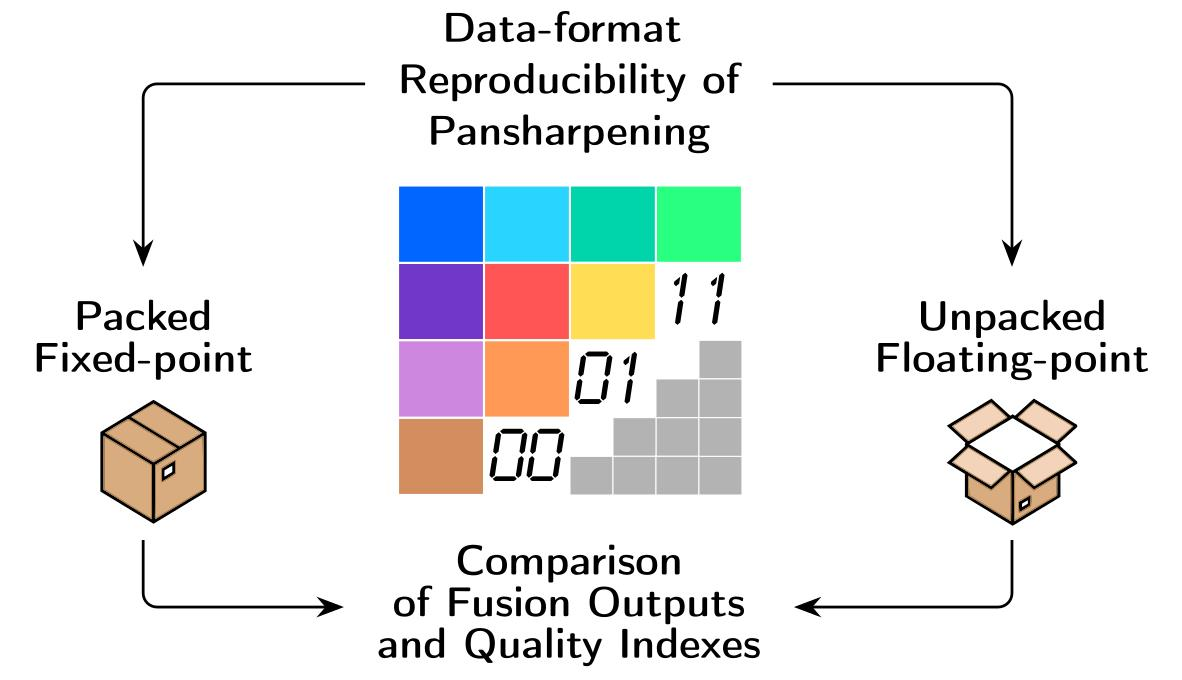
Remote sensing image data are generally available in packed fixed-point formats, together with floating-point gains and offsets, a pair for each band of each scene, that allow floating-point calibrated values to be recovered [17]. While the maximum value of each band of the scene is mapped onto the largest digital number (DN) of the fixed-point representation, offsets are generally set equal to the minimum value, such that the active range of floating-point values of the scene is exactly mapped onto the dynamic range of the DN representation. If the offsets are taken all equal to zero, the DN and the floating-point representations differ only by a scaling factor, which, however, may be different from one band to another in the same scene, thereby originating an alteration in the spectral content of the data.
A problem seldom investigated in the literature is whether it makes difference if fusion is accomplished in the packed DN format or in the original floating-point format. In this work, we are concerned with how the performance of pansharpening methods depends on their input data format. It is theoretically proven and experimentally demonstrated that MRA methods are unaffected by the data format, which instead is crucial for CS methods, unless their intensity component is calculated by means of a multivariate linear regression between the upsampled bands and the lowpass-filtered Pan, as it is accomplished by the most advanced CS methods, e.g., [18].
Quality assessment of the pansharpened images is another debated problem. Notwithstanding achievements over the last years [19,20,21,22,23,24,25], the problem is still open, being inherently ill-posed. A further source of uncertainty, which has been explicitly addressed very seldomly [26], is that also the measured quality may depend on the data format. The quality check often entails the shortcoming of performing fusion with both MS and Pan datasets degraded at spatial resolutions lower than those of the originals, in order to use non-degraded MS originals as quality references [27]. In this study, several widespread with-reference (dis)similarity indexes are reviewed and discussed in terms of the reproducibility of their output values towards the data format. We wish to stress that in the present context the term quality represents the fidelity to a hypothetically available reference, and has no relationship with the intrinsic quality of the data produced by the instrument, which mainly depends on the modulation transfer function (MTF) of the multiband system and on the SNR, due to a mixed noise model, both photon and electronic [28,29].
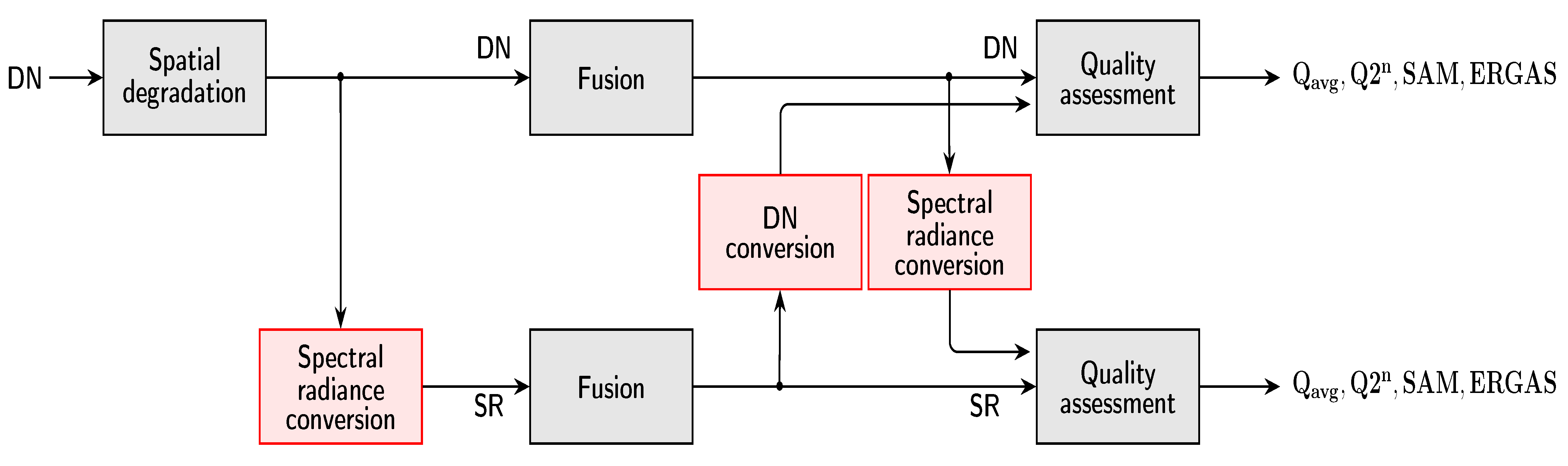
In an experimental setup, GeoEye-1 and WorldView-2 data are either fused in their packed 11-bits DN format or converted to spectral radiance before fusion is accomplished, by applying gain and offset metadata. In the former case, fusion results are converted to spectral radiance before quality is measured. In the latter case, fusion results are preliminarily converted to DNs. Results exactly match the theoretical investigations. For the majority of CS fusion methods, which do not feature a regression-based intensity calculation, results are better whenever they are obtained from floating-point data. Furthermore, the assessment of nine pansharpened products from as many algorithms, carried out both on floating-point and on packed fixed-point data, reveals that the quality evaluations may be misleading whenever they are performed on fixed-point DN formats.

2. Data Formats and Products

Remote sensing optical data, specifically MS and Pan, are available in spectral radiance format, that is radiance normalized to the width of the spectral interval of the imaging instrument, and in reflectance formats. The reflectance, which is implicitly spectral, ranges in [0,1] and can be defined either as top-of-atmosphere (TOA) reflectance or as surface reflectance, also called bottom-of-atmosphere (BOA) reflectance, if it is measured at sea level. The former is the reflectance as viewed by the satellite and is given by the TOA spectral radiance rescaled by the TOA spectral irradiance of the Sun. The latter represents the spectral signature of the imaged surface; its determination requires the estimation, through parametric modeling and/or measurements, of the upward and downward transmittances of the atmosphere and of the upward scattered radiance at TOA, also known as path radiance [30].
Besides the TOA spectral radiance, which is a level-one (L1) product, the TOA reflectance, another L1 product, is generally available for systems featuring a nadiral acquisition and a global Earth coverage, like ASTER, Landsat 7 ETM+, Landsat 8 OLI, and Sentinel-2. On the contrary, extremely high resolution (EHR) systems (IKONOS, QuickBird, GeoEye-1, WorldView-2/3/4, Pléiades 1AB) perform sparse acquisitions with maneuverable acquisition angles and may not have the TOA reflectance format available. The surface reflectance is a level-two (L2) product and is distributed for global-coverage systems (OLI, Sentinel-2), only where an instrument network is available for atmospheric measurements [31], though it has been recently shown that robust estimates of surface reflectance can be achieved through the same data that shall be atmospherically corrected [32].
In order to store and distribute fixed-point data (typically 8 to 16 bits per pixel per band), more compact and practical than floating-point data, the spectral radiance/reflectance values are rescaled to fill the 256 to 65,536 digital number (DN) counts of the binary representation. A negative bias may be introduced to force the minimum radiance/reflectance value in the zero DN. If p denotes the wordlength of the fixed point representation and L m a x ( L m i n ) the maximum (minimum) spectral radiance value, the conversion rule to DN is:
DN = L L m i n L m a x L m i n × ( 2 p 1 ) + 0.5 .
For each band, the reciprocal of the scaling factor, i.e. ( L m a x L m i n ) / ( 2 p 1 ) , and the bias changed of sign, i.e., L m i n , which are generally different for each band, are placed in the file header as gain and offset metadata and are used to restore calibrated floating-point values from the DNs, which are identical for the three formats, spectral radiance, and reflectances; only gains and offsets change. In some cases, the offsets are set equal to zero, for all bands, including Pan, regardless of the actual minimum, L m i n , which implies that the minimum DN may be greater than zero. This strategy is generally pursued when the wordlength of the packed DN is 11 bits or more. In the following of this study, we will show that such a choice is highly beneficial for the reproducibility of pansharpening methods and quality indexes.
We wish to remark that the packaging of floating-point data into DNs does not penalize the original precision of the calibrated data, which are obtained starting from the integer samples produced by the on-board analog-to-digital converter (ADC). Thus, the calibrated samples exhibit a finite number of floating-point values, which can be accommodated in a DN of suitable wordlength, comparable to that of the ADC; generally one bit less, because the ADC span is designed to encompass the dark signal, which is removed before calibration, and to leave an allowance to prevent saturation.
Eventually, for the kth spectral channel, the following relationships hold between the floating-point calibrated data, TOA spectral radiance, L TOA , TOA reflectance, ρ TOA , and surface reflectance, ρ BOA , and the packed fixed-point DN format that is distributed:
L k TOA = α k · DN k + β k
ρ k TOA = α k TOA · DN k + β k TOA
ρ k BOA = α k BOA · DN k + β k BOA
in which the DN k s are the same for the three formats, while the gains, α k , and the offsets, β k , are constant over the scene and variable from one band to another, including Pan. In the case of TOA reflectance, α k TOA and β k TOA are equal to α k and β k divided by the the solar irradiance, which cannot be assumed spatially constant if the scene is large. Therefore, α k TOA and β k TOA are not constant over the whole scene, but on the sub-scenes of a partition, e.g. in square blocks. Analogous considerations hold for α k BOA and β k BOA . Without loss of generality, hereafter we will consider only the TOA spectral radiance in Equation (2a), which will be simply referred to as spectral radiance (SR). 
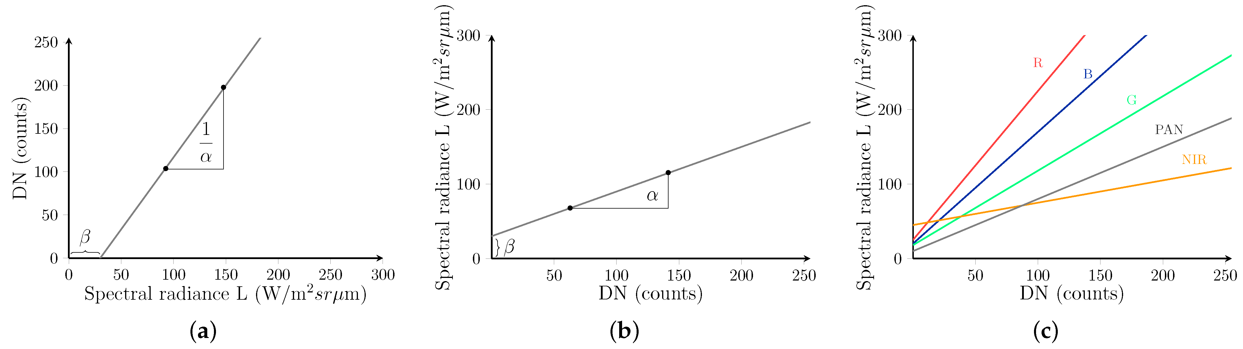
Figure 1a,b show the meaning of α and β : α is the slope and β the intercept of the inverse trans-characteristic that maps DN counts onto SR values. For the direct conversion in Figure 1a the slope is 1 / α and the intercept β / α . So, if gains and offsets are different for the bands of an MS image, including Pan, Figure 1c shows that the same DN value is mapped onto different values of SR depending on the band. Thus, there is a spectral alteration, a sort of miscalibration occurring if the DN counts are not converted back to physical units before their use. As it clearly appears from Figure 1c, such a miscalibration vanishes if gains and offsets are identical for each band, including Pan.

3. Basics of CS and MRA Pansharpening

Classical pansharpening methods can be divided into CS, MRA, and hybrid methods. The unique difference between CS and MRA is the way to extract the Pan details, either by processing the stack of bands along the spectral direction or in the spatial domain. Hybrid methods, e.g., [33,34], are the cascade of CS and MRA, either CS followed by MRA or, more seldom, MRA followed by CS. In the former case, they are equivalent to MRA that inherits the injection model from the CS; in the latter case, they behave like CS, with the injection model borrowed from MRA [8]. Therefore, at least for what concerns the present analysis, hybrid methods are not a third class with specific properties. The notation used in this paper will be firstly shown. Afterward, a brief review of CS and MRA will follow.

3.1. Notation

The math notation used is detailed in the following. Vectors are indicated in bold lowercase (e.g., x ) with the i-th element indicated as x i . 2-D and 3-D arrays are denoted in bold uppercase (e.g., X ). An MS image M = M k k = 1 , , N is a 3-D array composed by N spectral bands indexed by the subscript k. Accordingly, M k indicates the kth spectral band of M . The Pan image is a 2-D matrix indicated as P . The MS interpolated and pansharpened MS bands are denoted as M ˜ k and M ^ k , respectively. Unlike conventional matrix product and ratio, such operations are intended as product and ratio of terms of the same positions within the array.

3.2. CS

The class of CS, or spectral, methods is based on the projection of the MS image into another vector space, by assuming that the forward transformation splits the spatial structure and the spectral diversity into separate components. The problem may be stated as how to find the color space that is most suitable for fusion [35].
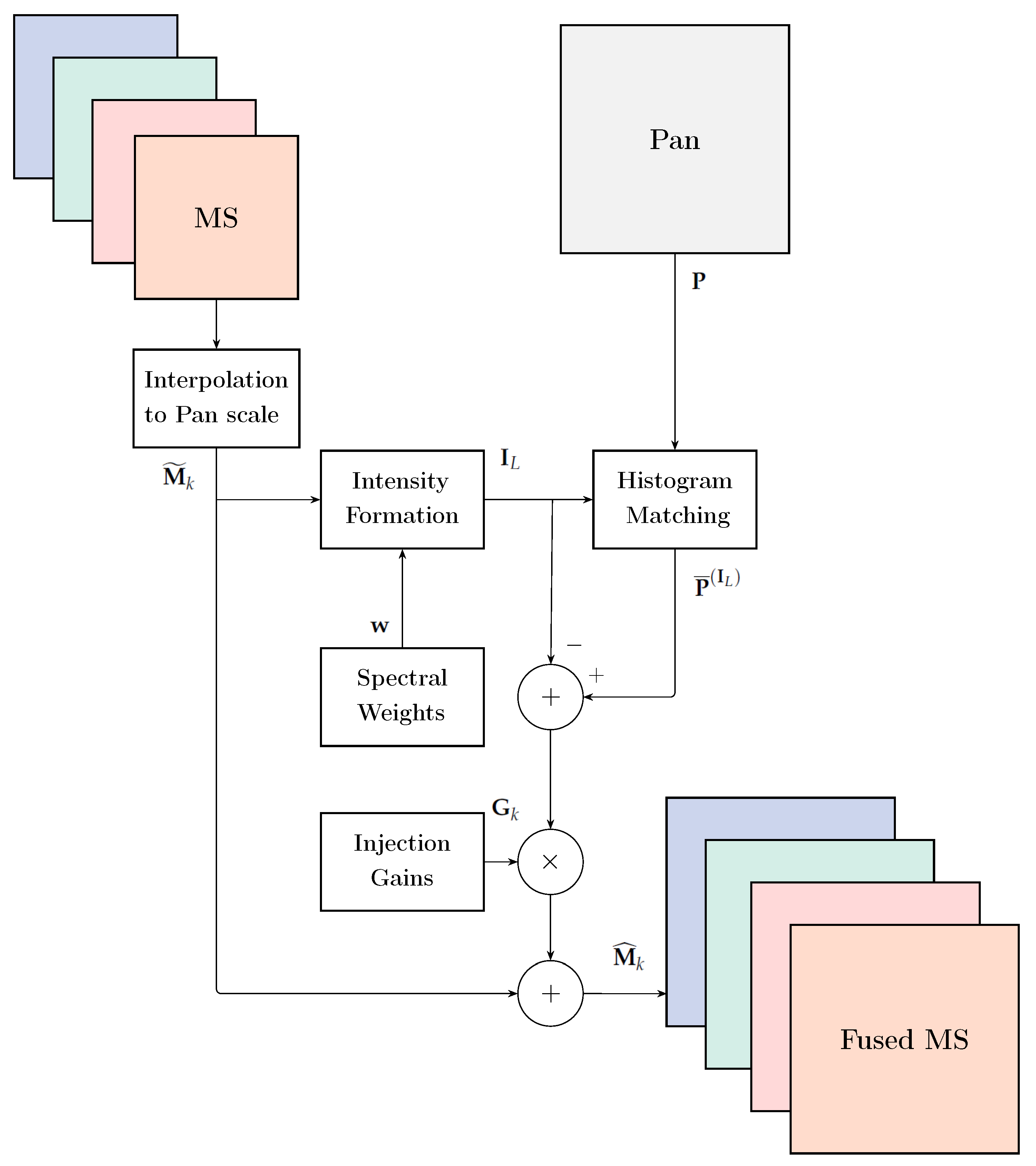
Under the hypothesis of substitution of a single component that is a linear combination of the input bands, the fusion process can be obtained without the explicit calculation of the forward and backward transformations, but through a proper injection scheme, thereby leading to the fast implementations of CS methods, whose general formulation is [1]:
M ^ k = M ˜ k + G k · P ¯ ( I L ) I L , k = 1 , , N
in which k is the band index, G = [ G 1 , , G k , , G N ] the 3-D array of injection gains, which in principle may be different for each pixel each band, while the intensity, I L , is defined as
I L = i = 1 N w i · M ˜ i
in which the weight vector w = [ w 1 , , w i , , w N ] is the 1-D array of spectral weights, corresponding to the first row of the forward transformation matrix [1]. The term P ¯ ( I L ) is P histogram-matched to I L
P ¯ ( I L ) ( P μ P ) · σ I L σ P L + μ I L
in which μ and σ denote mean and square root of variance, respectively, and P L is a lowpass version of P having the same spatial frequency content as I L [8]. Figure 2 shows the typical flowchart employed by CS methods.
The simplest CS fusion method is the Intensity-Hue-Saturation (IHS) [1], or better its generalization to an arbitrary number of bands, GIHS, which allows a fast implementation, given by Equation (3) with unitary injection gains, G k = 1 . The multiplicative or contrast-based injection model is a special case of Equation (3), in which space-varying injection gains, G , are defined such that
G k = M ˜ k I L , k = 1 , , N .
The resulting pansharpening method is described by
M ^ k = M ˜ k + M ˜ k I L · ( P ¯ ( I L ) I L ) = M ˜ k · P ¯ ( I L ) I L , k = 1 , , N
which, in the case of spectral weights all equal to 1 / N , is the widely known Brovey transform (BT) pansharpening method [1,36].
In Gram–Schmidt (GS) [37] spectral sharpening, the fusion process is described by Equation (3), where the injection gains are spatially uniform for each band, and thus denoted as g k k = 1 , , N . They are given by [8]:
g k = cov ( M ˜ k , I L ) var ( I L ) k = 1 , , N
in which cov X , Y indicates the covariance between X and Y , and var Y is the variance of Y . A multivariate linear regression has been exploited to model the relationship between the lowpass-filtered Pan, P L , and the interpolated MS bands [1,18],
P L = i = 1 N w ^ i · M ˜ i + b ^ + ϵ I ^ L + ϵ
in which I ^ L is the optimal intensity component and ϵ the least squares (LS) space-varying residue. The set of space-constant optimal weights, { w ^ k } k = 1 , , N , and b ^ , is calculated as the minimum MSE (MMSE) solution of Equation (9). A figure of merit of the matching achieved by the MMSE solution is given by the coefficient of determination (CD), namely R 2 , defined as
R 2 1 σ ϵ 2 σ P L 2
in which σ ϵ 2 and σ P L 2 denote the variance of the (zero-mean) LS residue, ϵ , and of the lowpass-filtered Pan image, respectively. Histogram-matching of Pan to the MMSE intensity component, I ^ L , should take into account that μ P = μ P L = μ I ^ L , from Equation (9). Thus, from the definition of CD in Equation (10)
P ¯ ( I ^ L ) = ( P μ P ) · R + μ P .
This brief review does not include a popular CS fusion method employing principal component analysis (PCA). The reason is that PCA is a particular case of the more general GS transformation, in which I L is equal to the maximum-variance first principal component, PC1, and the injection gains are those of GS, as in Equation (8), [1].

3.3. MRA

The 
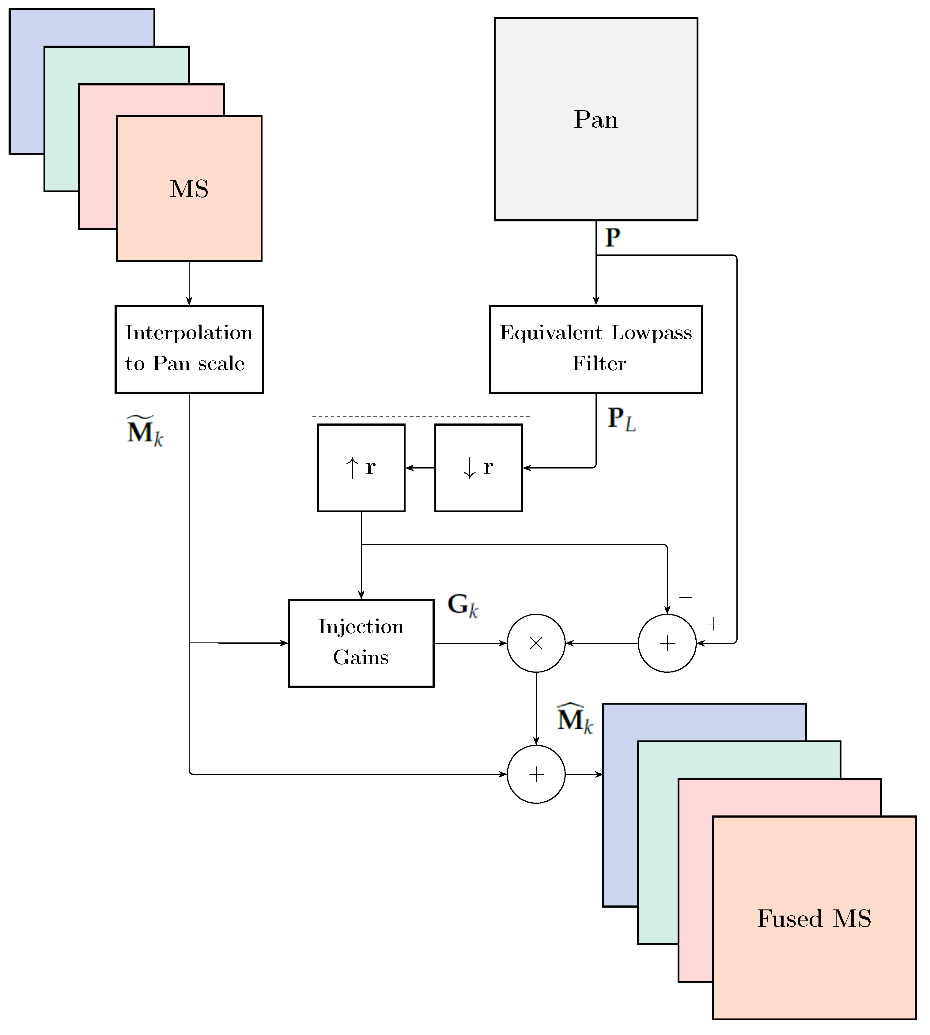
spatial approach relies on the injection of highpass spatial details of Pan into the resampled MS bands. The most general MRA-based fusion may be stated as:
M ^ k = M ˜ k + G k · P ¯ ( M ˜ k ) P ¯ L ( M ˜ k ) , k = 1 , , N .
in which the Pan image is preliminarily histogram-matched to the interpolated kth MS band [8]
P ¯ ( M ˜ k ) ( P μ P ) · σ M ˜ k σ P L + μ M ˜ k
and P ¯ L ( M ˜ k ) the lowpass-filtered version of P ¯ ( M ˜ k ) . It is noteworthy that according to either of Equations (5) and (13), histogram matching of P always implies the calculation of its lowpass version P L .
According to Equation (12) the different approaches and methods belonging to this class are uniquely characterized by the lowpass filter employed for obtaining the image P L , by the presence or absence of a decimator/interpolator pair [38] and by the set of space-varying injection gains, either spatially uniform, g k k = 1 , , N or space-varying, G k k = 1 , , N . The contrast-based version of MRA pansharpening is
M ^ k = M ˜ k + M ˜ k P ¯ L ( M ˜ k ) · P ¯ ( M ˜ k ) P ¯ L ( M ˜ k ) = M ˜ k · P ¯ ( M ˜ k ) P ¯ L ( M ˜ k ) , k = 1 , , N .
It is noteworthy that, unlike what happens for Equation (7), Equation (14) does not preserve the spectral angle of M ˜ k , because the multiplicative sharpening term depends on k, through Equation (13). Eventually, the projective injection gains derived from GS (Equation (8)) can be extended to MRA fusion as
g k = cov ( M ˜ k , P L ) var ( P L ) k = 1 , , N
whose space varying-version G k , with statistics calculated locally on a sliding window, coupled with a pyramid MRA constitutes a popular pansharpening method known as GLP-CBD [1,39]. Figure 3 shows the general flowchart of spatial, a.k.a. MRA, pansharpening methods.

4. Reproducibility of Results of Pansharpening Methods with the Data Format

Here, we derive the conditions that allow CS and MRA pansharpening methods to attain reproducibility with the input data format. In particular, we will refer to the case of SR, even though the proof is also valid for reflectance formats:
P S R = α P · P D N + β P M ˜ k S R = α k · M ˜ k D N + β k , k = 1 , , N
in which the superscripts SR and DN indicate that the quantity is expressed in SR units (floating-point) or in DN (fixed-point), respectively.
Upon these premises, we consider a pansharpening method to be reproducible vs. data-format if:
M ^ k S R = α k · M ^ k D N + β k , k = 1 , , N
or, equivalently, if the fusion process preserves the linear affine transformation of the data-format conversion.

4.1. CS

The analysis of data-format reproducibility of CS methods is more complicated than that of MRA methods because the spectral bands are combined together to produce the intensity component, unlike the band-to-band processing of MRA. Let us start from the general form of CS methods in Equation (3), considering the projective injection of coefficients of Equation (8) and the intensity component with spectral weights calculated as MMSE solution of Equation (9):
M ^ k S R = M ˜ k S R + g k S R · P ¯ ( I ^ L S R ) S R I ^ L S R , k = 1 , , N ,
in which
I ^ L S R = i = 1 N w ^ i S R · M ˜ i S R + b ^ S R .
From the LS solution of Equation (9), it is easily proven that the following relationships hold between spectral weights and bias terms in DN and in SR formats:
w ^ k S R = w ^ k D N · α P α k , k = 1 , , N b ^ S R = α P · b ^ D N + β P α P · i = 1 N w ^ i D N · β i α i R S R = R D N = R
It is noteworthy that the degree of matching achieved by the LS solution, given by Equation (10), is identical for the two formats. Substituting Equation (20) into Equation (19) yields the relationship between SR and DN intensity components:
I ^ L S R = i = 1 N w ^ i S R · M ˜ i S R + b ^ S R = i = 1 N w ^ i D N · α P α i · ( α i · M ˜ i D N + β i ) + α P · b ^ D N + β P α P · i = 1 N w ^ i D N · β i α i = α P · ( i = 1 N w ^ i D N · M ˜ i D N + b ^ D N ) + β P = α P · I ^ L D N + β P
Hence, the histogram-matching of Pan to I ^ L S R in Equation (11), becomes:
P ¯ ( I ^ L S R ) S R = ( P S R μ P S R ) · R + μ P S R = α P · ( P D N + β P / α P μ P D N β P / α P ) · R + μ P D N + β P = α P · P ¯ ( I ^ L D N ) D N + β P .
Furthermore, the SR and DN injections gains can be related as:
g k S R = cov ( M ˜ k S R , I ^ L S R ) var ( I ^ L S R ) = α k α P · cov ( M ˜ k D N , I ^ L D N ) var ( I ^ L D N ) = α k α P · g k D N .
Finally, substituting Equations (21)-(22)-(23) into Equation (18), we obtain:
M ^ k S R = M ˜ k S R + g k S R · P ¯ ( I ^ L S R ) S R I ^ L S R = α k · M ˜ k D N + β k + α k α P · g k D N · α P · P ¯ ( I ^ L D N ) D N I ^ L D N = α k · M ^ k D N + β k .
It is important to remark that Equation (24) holds only if the relationships of Equation (20) are satisfied, which implicitly happens to regression-based CS methods. The unitary injection gain (GIHS) does not affect the reproducibility of fusion if Equation (20) holds. Conversely, it is easily proven that, when the offsets are nonzero, the multiplicative injection model of Equation (6) is never reproducible also if Equation (9), and hence Equation (20), hold. In summary, for CS methods, the key to achieve data-format reproducibility lies in the relationships of Equation (20) between the spectral weights calculated in the different data formats, which is implicitly satisfied if the intensity component is calculated as in Equation (9).

4.2. MRA

Starting from Equation (12), we firstly focus on the detail term and thus set the band-dependent injection gains all equal to unity:
M ^ k S R = M ˜ k S R + P ¯ ( M ˜ k S R ) S R P ¯ L ( M k S R ) S R , k = 1 , , N .
Starting from Equation (16), the relationship between histogram-matched Pan, in either DN or SR format, can be written as:
P ¯ ( M ˜ k S R ) S R = ( P S R μ P S R ) · σ M ˜ k S R σ P L S R + μ M ˜ k S R = α P · ( P D N + β P / α p μ P D N β P / α P ) · α k α P · σ M ˜ k D N σ P L D N + α k · μ M ˜ k D N + β k = α k · P ¯ ( M ˜ k D N ) D N + β k
where we have used the following relationships for the mean and standard deviation:
μ P S R = α P · μ P D N + β P , σ P L S R = α P · σ P L D N μ M ˜ k S R = α k · μ M ˜ k D N + β k , σ M ˜ k S R = α k · σ M ˜ k S R , k = 1 , , N .
Finally, Equation (25) can be rewritten as:
M ^ k S R = α k · M ˜ k D N + β k + α k · P ¯ ( M ˜ k D N ) D N + β k / α k P ¯ L ( M ˜ k D N ) D N β k / α k = α k · M ^ k D N + β k , k = 1 , , N .
In the case of non-unitary injection gains, such as the projective and the multiplicative coefficients, it is easily proven that the former is independent of the format, analogously to Equation (23); the latter only if the offsets are zero. In summary, the key to data-format reproducibility of MRA methods lies in the band-by-band linear histogram matching operation of Equation (13), thanks to which the sharpening Pan inherits gain and offset from the MS band that shall be sharpened.

5. Reproducibility of Quality Indexes Varying with Data Formats

In this section, the most popular statistical similarity/dissimilarity indexes, suitable for multiband images, will be reviewed and their behavior for DN and calibrated data formats will be investigated.

5.1. SAM

Spectral angle mapper (SAM) was originally introduced for the discrimination of materials starting from their reflectance spectra [40]. Given two spectral vectors, v and v ^ , both having N components, in which v = { v 1 , v 2 , , v N } is the reference spectral pixel vector and v ^ = { v ^ 1 , v ^ 2 , , v ^ N } is the test spectral pixel vector, SAM denotes the absolute value of the spectral angle between the two vectors:
SAM ( v , v ^ ) arccos < v , v ^ > | | v | | 2 · | | v ^ | | 2 .
SAM is usually expressed in degrees and is equal to zero iff the test vector is spectrally identical to the reference vector, i.e., the two vectors are parallel and may differ only by their moduli. A global spectral dissimilarity, or distortion, index is obtained by averaging Equation (29) over the scene. From Equation (2) it is evident that whether Equation (29) is calculated with the two vectors in DN or SR, makes a difference. The angle measured in the two formats is identical if the offsets, β k , are all zero and the gains, α k , are the same for each band. Whenever this does not occur, the angle measured by Equation (29) is different for the two formats, which is a reasonable conclusion for a spectral distortion measure.

5.2. ERGAS

ERGAS, the French acronym for relative dimensionless global error in synthesis [41], is a normalized dissimilarity index that offers a global indication of the distortion towards the reference of a test multiband image, as produced by a pansharpening method:
ERGAS 100 d h d l 1 N k = 1 N RMSE ( k ) μ ( k ) 2
where d h / d l is the ratio between pixel sizes of Pan and MS, e.g., 1/4, μ ( k ) is the mean (average) of the kth band of the reference and N is the number of bands. Low values of ERGAS indicate high similarity between fused and reference MS data. Since ERGAS is nothing more than the cumulative normalized root mean square error (NRMSE), multiplied by the Pan-to-MS scale ratio and expressed in percentage, its value is insensitive to changes in the spectral gains, α k , of individual bands. Instead, the presence of nonzero band offsets, β k , produces lower values of the mean, μ ( k ) , and hence values of ERGAS higher than those with offsets that are all equal to zero.

5.3. Multivariate UIQI

Q 2 n is the multiband extension of the universal image quality index (UIQI) [42] and was introduced for quality assessment of pansharpened MS images [43]. Each pixel of an image with N spectral bands is accommodated into a hypercomplex (HC) number with one real part and N 1 imaginary parts.
Let z = z ( m , n ) and z ^ = z ^ ( m , n ) denote the HC representation of the reference and test spectral vectors at pixel ( m , n ) . Analogously to UIQI, namely, Q 2 0 = Q, Q 2 n may be written as the product of three terms:
Q 2 n = | σ z z ^ | σ z σ z ^ · 2 σ z σ z ^ σ z 2 + σ z ^ 2 · 2 | z ¯ | | z ^ ¯ | | z ¯ | 2 + | z ^ ¯ | 2
the first of which is the modulus of the HC correlation coefficient (HCCC) between z and z ^ . The second and third terms, respectively, measure contrast changes and mean bias on all bands simultaneously. Statistics are calculated on square blocks, typically, 32 × 32, and Q 2 n is averaged over the blocks of the whole image to yield the global score index. Q 2 n takes values in [0,1] and is equal to 1 iff z = z ^ for all pixels. From the definitions of mean, variance, and covariance of HC random variables, it can be proven that the covariance, and hence the HCCC, is sensitive to gains, α k , but only if such gains are not equal for all bands. The contrast-change term is always insensitive to offsets, but not to band-varying gains. In the presence of nonzero band offsets, β k , also the mean-bias term may change.
Analogously, it can be easily proven that the univariate index UIQI, often calculated on the individual bands and averaged to yield a unique quality index, is independent of any choice of gains, also different from one another, but is affected by the presence of offsets, also equal to one another.
In conclusion, while ERGAS and average UIQI are independent of gains, whichever they are, all the four indexes measure different values for the two formats, in the presence of offsets, also equal to one another.

6. Experimental Results and Discussion

6.1. Data Sets

Two test images, acquired by two different platforms, GeoEye-1 and WorldView-2, have been used in the simulations. In this section, besides describing the two datasets, we propose an index to measure the spectral alteration of the DN representation and present an analysis of the solution of the multivariate regression of Equation (9) for the two datasets.

6.1.1. Collazzone Dataset

The GeoEye-1 image has been acquired over the area of Collazzone, a rural locality in Central Italy, on 13 July 2010. The spatial sampling interval (SSI) is 2 m for MS and 0.5 m for Pan, resulting in a scale ratio equal to four. The MS image features four spectral bands: blue (B), green (G), red (R) and near infra-red (NIR). The image size is 512 × 512 pixels for MS and 2048 × 2048 for Pan. The radiometric resolution of the DN format is 11 bits; the conversion coefficients to the SR format, extracted from the metadata, are reported in Table 1. It is noteworthy that the offsets are all equal to zero.

6.1.2. Sydney Dataset

The WorldView-2 image, acquired on 21 August 2012, portrays the city of Sydney, Australia. The SSI is 2 m for MS and 0.5 m for Pan; hence, the scale ratio is still four. The MS image comprises eight bands: coastal (C), B, G, yellow (Y), R, red edge (RE), NIR1, and NIR2. The covered area is 1,048,576 m 2 , corresponding to MS and Pan image sizes of 512 × 512 and 2048 × 2048 pixels, respectively. The fixed-point representation of the data employs 11 bits. Table 2 shows the corresponding radiometric calibration coefficients obtained from the metadata file. Also in this case the offsets are identically equal to zero.

6.2. Spectral Imbalance Factor

The conversion to SR of DN counts in Equation (2a) has the effect of restoring the original spectral inter-relationships of the calibrated data that have been lost after integer packaging. In other words, the integer-valued samples may be spectrally altered, if the gains and/or offsets are not equal to one another. A measure of such a spectral alteration can be defined as spectral imbalance factor (SIF):
SIF % α m a x α m i n α m a x · exp β m a x β m i n β m a x + c × 100
where α m i n ( β m i n ) and α m a x ( β m a x ) are respectively the minimum and the maximum values of the gains (offsets) of the spectral bands, including Pan; c a machine tolerance to avoid zero-by-zero divisions. SIF% is zero iff the α k , including α P , are equal to one another and is independent of the offsets iff they are equal to one another, also if they are all zero. As reported in Table 1 and Table 2, SIF% is equal to 65.35% for the Collazzone dataset and 60.89% for the Sydney dataset. The presence of nonzero offsets would increase SIF%, as it appears from Equation (32). Note that, for both datasets, the minimum gain is that of the NIR channel (NIR2 for WorldView-2), the maximum gain is on the red channel for Collazzone and on the blue one for Sydney, which means that the red/blue bands have been the most compressed, in order to fit the 11-bit DN representation; the NIR/NIR2 bands, the least.

6.3. Analysis of the LS Intensity Component

The LS solution of the multivariate linear regression of Equation (9) is now discussed for the two test datasets. Table 3 and Table 4 report the MMSE spectral weights of each band and the bias coefficient, when it is included or not, for both the DN and the SR formats. All the experimental values match the theoretical investigations of Equation (20); in particular, the CD, also called R 2 , is identical for the two formats. The presence or absence of the bias term produces w ^ k somewhat different in the two cases, but this has a very limited impact on the degree of matching, measured by CD, which changes on the fourth decimal digit. This happens because in both the test images offsets are not present, i.e., they are identically zero. In the presence of nonzero offsets, the regression must include the bias term, which compensates for the offsets of the DN format, according to Equation (20). Note that the sum of the spectral weights slightly exceeds one, in all cases, less for GE-1 than for WV-2. This result is in agreement with the layout of spectral bands of the two instruments, since weights summing to one would indicate that the spectral width of Pan is equal to the total span of the accompanying MS bands.

6.4. Simulations

Nine pansharpening algorithms, including the plain interpolated MS image, without injection of details, denoted by EXP, have been selected from the Pansharpening Toolbox [39]. Figure 4 shows the flowchart of the experimental setup. The goal is twofold: (i) to determine the possible dependence of quality assessment metrics on the specific data format, in which they are evaluated; (ii) to check which pansharpening methods perform identically, regardless of the data format. After the original MS + Pan dataset has been spatially degraded, all fusion methods are run twice: once on the DN data and once on the DN data preliminarily converted to SR. In this way, two sets of fused images are made available, one in DN and one in SR. Each fused dataset is then converted to the other format: the output of the fusion process in DN is converted to SR and the output of fusion in SR is converted back to DN. This procedure allows reproducibility of methods and reproducibility of indexes to be evaluated in a unique simulation session. Thus, data-format reproducible pansharpening methods and data-format reproducible quality indexes are jointly identified.
Table 5 and Table 6 report the numerical results of the simulations performed on the two datasets. The organization of the tables requires some explications. Each table is composed of two subtables: the upper one reports the values of quality indexes calculated on data in DN format; the lower subtable reports the same quality metrics calculated in SR format. The cell in each table contains two values: the left term refers to fusion performed in DN; the right one to fusion in SR. In order to check whether a quality index is invariant towards the data format or not, it is sufficient to check whether the columns in the two subtables relative to the same index are identical or not.
The data-format reproducible quality/distortion indexes have been marked with a green bullet beside a down arrow, while the non-reproducible ones with a red bullet beside a down arrow. The upper and lower matching columns are highlighted in light green; the columns of non-reproducible indexes are highlighted in light red. Therefore, average UIQI and ERGAS are format-reproducible; multivariate UIQI and SAM are not. These results match the theoretical investigations, because the offsets are all zero. Otherwise, none of the indexes would be reproducible. Analogously, in order to check the data-format reproducibility of a pansharpening method, we need to look at rows instead of columns. For a given method, if the two values inside every cell of the row are identical to each other, the pansharpening method is data-format reproducible; otherwise, it is not. Data-format reproducible methods are marked with a green square beside a right arrow; non-reproducible methods with red square and arrow. We can verify that all MRA methods (ATWT and MTF-GLP) and some CS methods (GSA and BDSD) provide results invariant with the data format. Conversely, all first-generation CS pansharpening methods, such as GS, GIHS, BT, and PCA, provide different results depending on the input data format. The experimental results match the theoretical investigations presented in Section 4, within the limits that both the available test datasets have zero offsets. In the presence of nonzero offsets. Incidentally, since M ^ k = M ˜ k , EXP is, by its definition, format-reproducible. Note that, for methods that are not reproducible, results are always better whenever the algorithms are run on data in SR format.
The results of the fusion process at reduced resolution for each of the methods are shown in Figure 5 and Figure 6, for the datasets of Collazzone and Sydney, respectively. For merely visual convenience, fusion is carried out in DNs and the results are displayed in the same format. This fact is not surprising, because the earlier SPOT data (G, R, NIR) were originally distributed in a packed 8-bit format, in order to be directly mapped onto displaying devices, which usually have 8 bits per color channel.

7. Concluding Remarks

In this work, we have investigated how the performance of a pansharpening method depends on the input data format, either packed DNs of Equation (1) or SR, as well as any other floating-point calibrated format. It is theoretically proven and experimentally demonstrated that MRA methods are unaffected by the data format, which instead is crucial for CS methods, unless their intensity component is calculated by means of a multivariate linear regression between the interpolated bands and the lowpass-filtered Pan, as it is accomplished by the most advanced CS methods. For CS fusion methods that do not feature a regression-based intensity calculation, results are better whenever they are obtained from floating-point data. For this reason, whenever the data that are merged come from different platforms [44] and/or are related to different intervals of the electromagnetic spectrum [45], the use of floating-point formats is highly recommended. This study has also demonstrated the necessary non-reproducibility versus the data format of normalized spectral similarity indexes for multiband images. This is necessary because if an index yields the same values when it is calculated from data in packed fixed-point or floating-point formats, it will not necessarily be a spectral index. Conversely, normalized spatial/radiometric indexes are those and only those that do not depend on the format of the data that are compared, at least if the band offsets are all zero. Thus, spectral similarity should be measured on data that are represented as physical units, e.g., SR. Use of packed DNs may lead to misestimation of quality, because DN data are spectrally altered, and hence miscalibrated, if the gains are not equal to one another and the offsets are nonzero.
A viable escape to retain the advantages of a fixed-point processing, mandatory for most of dedicated hardware implementations, and avoid the drawbacks of the spectral distortion, originated by the packaging of floating-point calibrated data of Equation (1), could be:
  • convert the available packed DNs to floating-point SR, or any other physical format, by using Equation (2a);
  • convert the SR data obtained at the previous step back to DN by using Equation (1), in which L m a x is not the maximum of the individual band of the scene, but of the whole scene, and L m i n = 0 .
Thus, it is easily verified that the gains α k are identical to one another and the offsets β k are all zero. Hence, it turns out that the distortion factor SIF%, Equation (32), is identically zero. As a final remark, notwithstanding that remote sensing data fusion by means of extremely sophisticated machine learning (ML) tools, e.g., [46], has nowadays reached the state of the art [2], the behaviors of such methods can be hardly modeled and hence predicted because they are based on the outcome of a complex learning process and not on simple constitutive relations. Consequently, it is not easy to prove or foresee if an ML fusion method trained on packed DN data gives the same results as the same method trained on floating-point spectral radiance data. Only an experimental analysis, as carried out in Section 6, would be feasible for ML-based pansharpening methods, but in this case, the analysis and its outcome would not be reproducible, thereby invalidating its motivations. Therefore it is recommended that all the training data are used in floating-point format and fusion is accomplished and assessed in the same format.

Author Contributions

Conceptualization and methodology: A.A., B.A., L.A. and A.G.; validation and software: A.A. and A.G.; data curation: A.A. and B.A.; writing: A.A. and L.A. All authors have read and agreed to the published version of the manuscript.

Funding

This research was financially supported in part by the Ph.D Course in Information Engineering, Cycle XXXIV, of the University of Florence.

Data Availability Statement

Not applicable.

Conflicts of Interest

The authors declare no conflict of interest.

References

  1. Alparone, L.; Aiazzi, B.; Baronti, S.; Garzelli, A. Remote Sensing Image Fusion; CRC Press: Boca Raton, FL, USA, 2015. [Google Scholar]
  2. Vivone, G.; Dalla Mura, M.; Garzelli, A.; Restaino, R.; Scarpa, G.; Ulfarsson, M.; Alparone, L.; Chanussot, J. A new benchmark based on recent advances in multispectral pansharpening: Revisiting pansharpening with classical and emerging pansharpening methods. IEEE Geosci. Remote Sens. Mag. 2021, 9, 53–81. [Google Scholar] [CrossRef]
  3. Arienzo, A.; Alparone, L.; Aiazzi, B.; Garzelli, A. Automatic fine alignment of multispectral and panchromatic images. In Proceedings of the 2020 IEEE International Geoscience and Remote Sensing Symposium (IGARSS), Waikoloa, HI, USA, 26 September–2 October 2020; pp. 228–231. [Google Scholar]
  4. Aiazzi, B.; Alparone, L.; Argenti, F.; Baronti, S. Wavelet and pyramid techniques for multisensor data fusion: A performance comparison varying with scale ratios. In Proceedings of the SPIE Image Signal Processing Remote Sensing V, Florence, Italy, 20–24 September 1999; Serpico, S.B., Ed.; Volume 3871, pp. 251–262. [Google Scholar]
  5. Garzelli, A.; Nencini, F.; Alparone, L.; Baronti, S. Multiresolution fusion of multispectral and panchromatic images through the curvelet transform. In Proceedings of the 2005 IEEE International Geoscience and Remote Sensing Symposium (IGARSS), Seoul, Korea, 24–29 July 2005; pp. 2838–2841. [Google Scholar]
  6. Baronti, S.; Aiazzi, B.; Selva, M.; Garzelli, A.; Alparone, L. A theoretical analysis of the effects of aliasing and misregistration on pansharpened imagery. IEEE J. Sel. Top. Signal Process. 2011, 5, 446–453. [Google Scholar] [CrossRef]
  7. Aiazzi, B.; Alparone, L.; Baronti, S.; Carlà, R.; Garzelli, A.; Santurri, L. Sensitivity of pansharpening methods to temporal and instrumental changes between multispectral and panchromatic data sets. IEEE Trans. Geosci. Remote Sens. 2017, 55, 308–319. [Google Scholar] [CrossRef]
  8. Alparone, L.; Garzelli, A.; Vivone, G. Intersensor statistical matching for pansharpening: Theoretical issues and practical solutions. IEEE Trans. Geosci. Remote Sens. 2017, 55, 4682–4695. [Google Scholar] [CrossRef]
  9. Vivone, G.; Marano, S.; Chanussot, J. Pansharpening: Context-based generalized Laplacian pyramids by robust regression. IEEE Trans. Geosci. Remote Sens. 2020, 58, 6152–6167. [Google Scholar] [CrossRef]
  10. Li, H.; Jing, L. Improvement of a pansharpening method taking into account haze. IEEE J. Sel. Top. Appl. Earth Observ. Remote Sens. 2017, 10, 5039–5055. [Google Scholar] [CrossRef]
  11. Lolli, S.; Alparone, L.; Garzelli, A.; Vivone, G. Haze correction for contrast-based multispectral pansharpening. IEEE Geosci. Remote Sens. Lett. 2017, 14, 2255–2259. [Google Scholar] [CrossRef]
  12. Garzelli, A.; Aiazzi, B.; Alparone, L.; Lolli, S.; Vivone, G. Multispectral pansharpening with radiative transfer-based detail-injection modeling for preserving changes in vegetation cover. Remote Sens. 2018, 10, 1308. [Google Scholar] [CrossRef] [Green Version]
  13. Vivone, G.; Alparone, L.; Garzelli, A.; Lolli, S. Fast reproducible pansharpening based on instrument and acquisition modeling: AWLP revisited. Remote Sens. 2019, 11, 2315. [Google Scholar] [CrossRef] [Green Version]
  14. Addesso, P.; Longo, M.; Restaino, R.; Vivone, G. Sequential Bayesian methods for resolution enhancement of TIR image sequences. IEEE J. Sel. Top. Appl. Earth Observ. Remote Sens. 2015, 8, 233–243. [Google Scholar] [CrossRef]
  15. Aiazzi, B.; Alparone, L.; Arienzo, A.; Garzelli, A.; Zoppetti, C. Monitoring of changes in vegetation status through integration of time series of hyper-sharpened Sentinel-2 red-edge bands and information-theoretic textural features of Sentinel-1 SAR backscatter. In Image and Signal Processing for Remote Sensing XXV; Bruzzone, L., Ed.; International Society for Optics and Photonics: Bellingham, WA, USA, 2019; Volume 11155, p. 111550Z. [Google Scholar]
  16. Aiazzi, B.; Alparone, L.; Baronti, S. Information-theoretic heterogeneity measurement for SAR imagery. IEEE Trans. Geosci. Remote Sens. 2005, 43, 619–624. [Google Scholar] [CrossRef]
  17. Schowengerdt, R.A. Remote Sensing: Models and Methods for Image Processing, 2nd ed.; Academic Press: Orlando, FL, USA, 1997. [Google Scholar]
  18. Vivone, G. Robust band-dependent spatial-detail approaches for panchromatic sharpening. IEEE Trans. Geosci. Remote Sens. 2019, 57, 6421–6433. [Google Scholar] [CrossRef]
  19. Aiazzi, B.; Alparone, L.; Baronti, S.; Carlà, R. Assessment of pyramid-based multisensor image data fusion. In SPIE Image Signal Processing Remote Sensing IV; Serpico, S.B., Ed.; International Society for Optics and Photonics: Bellingham, WA, USA, 1998; Volume 3500, pp. 237–248. [Google Scholar]
  20. Du, Q.; Younan, N.H.; King, R.L.; Shah, V.P. On the performance evaluation of pan-sharpening techniques. IEEE Geosci. Remote Sens. Lett. 2007, 4, 518–522. [Google Scholar] [CrossRef]
  21. Aiazzi, B.; Alparone, L.; Baronti, S.; Carlà, R.; Garzelli, A.; Santurri, L. Full scale assessment of pansharpening methods and data products. In SPIE Image Signal Processing Remote Sensing XX; Bruzzone, L., Ed.; International Society for Optics and Photonics: Bellingham, WA, USA, 2014; Volume 9244, p. 924402. [Google Scholar]
  22. Carlà, R.; Santurri, L.; Aiazzi, B.; Baronti, S. Full-scale assessment of pansharpening through polynomial fitting of multiscale measurements. IEEE Trans. Geosci. Remote Sens. 2015, 53, 6344–6355. [Google Scholar] [CrossRef]
  23. Alparone, L.; Garzelli, A.; Vivone, G. Spatial consistency for full-scale assessment of pansharpening. In Proceedings of the 2018 IEEE International Geoscience and Remote Sensing Symposium (IGARSS), Valencia, Spain, 22–27 July 2018; pp. 5132–5134. [Google Scholar]
  24. Vivone, G.; Restaino, R.; Chanussot, J. A Bayesian procedure for full resolution quality assessment of pansharpened products. IEEE Trans. Geosci. Remote Sens. 2018, 56, 4820–4834. [Google Scholar] [CrossRef]
  25. Agudelo-Medina, O.; Benitez-Restrepo, H.; Vivone, G.; Bovik, A. Perceptual quality assessment of pan-sharpened images. Remote Sens. 2019, 11, 877. [Google Scholar] [CrossRef] [Green Version]
  26. Arienzo, A.; Alparone, L.; Aiazzi, B.; Baronti, S.; Garzelli, A. Reproducibility of spectral and radiometric normalized similarity indices for multiband images. In Proceedings of the 2019 IEEE International Geoscience and Remote Sensing Symposium (IGARSS), Yokohama, Japan, 28 July–2 August 2019; pp. 839–842. [Google Scholar]
  27. Palsson, F.; Sveinsson, J.R.; Ulfarsson, M.O.; Benediktsson, J.A. Quantitative quality evaluation of pansharpened imagery: Consistency versus synthesis. IEEE Trans. Geosci. Remote Sens. 2016, 54, 1247–1259. [Google Scholar] [CrossRef]
  28. Aiazzi, B.; Alparone, L.; Barducci, A.; Baronti, S.; Pippi, I. Estimating noise and information of multispectral imagery. Opt. Eng. 2002, 41, 656–668. [Google Scholar]
  29. Alparone, L.; Selva, M.; Capobianco, L.; Moretti, S.; Chiarantini, L.; Butera, F. Quality assessment of data products from a new generation airborne imaging spectrometer. In Proceedings of the 2009 IEEE International Geoscience and Remote Sensing Symposium (IGARSS), Cape Town, South Africa, 12–17 July 2009; Volume IV, pp. IV422–IV425. [Google Scholar]
  30. Pacifici, F.; Longbotham, N.; Emery, W.J. The importance of physical quantities for the analysis of multitemporal and multiangular optical very high spatial resolution images. IEEE Trans. Geosci. Remote Sens. 2014, 52, 6241–6256. [Google Scholar] [CrossRef]
  31. Lolli, S.; Di Girolamo, P. Principal component analysis approach to evaluate instrument performances in developing a cost-effective reliable instrument network for atmospheric measurements. J. Atmos. Ocean. Technol. 2015, 32, 1642–1649. [Google Scholar] [CrossRef]
  32. Bilal, M.; Nazeer, M.; Nichol, J.; Bleiweiss, M.; Qiu, Z.; Jakel, E.; Campbell, J.; Atique, L.; Huang, X.; Lolli, S. A simplified and robust surface reflectance estimation method (SREM) for use over diverse land surfaces using multi-sensor data. Remote Sens. 2019, 11, 1344. [Google Scholar] [CrossRef] [Green Version]
  33. Shah, V.P.; Younan, N.H.; King, R.L. An efficient pan-sharpening method via a combined adaptive-PCA approach and contourlets. IEEE Trans. Geosci. Remote Sens. 2008, 46, 1323–1335. [Google Scholar] [CrossRef]
  34. Licciardi, G.; Vivone, G.; Dalla Mura, M.; Restaino, R.; Chanussot, J. Multi-resolution analysis techniques and nonlinear PCA for hybrid pansharpening applications. Multidim. Syst. Signal Process. 2016, 27, 807–830. [Google Scholar] [CrossRef]
  35. Aiazzi, B.; Alparone, L.; Arienzo, A.; Garzelli, A.; Lolli, S. Fast multispectral pansharpening based on a hyper-ellipsoidal color space. In Image and Signal Processing for Remote Sensing XXV; Bruzzone, L., Ed.; International Society for Optics and Photonics: Bellingham, WA, USA, 2019; Volume 11155, p. 1115507. [Google Scholar]
  36. Gillespie, A.R.; Kahle, A.B.; Walker, R.E. Color enhancement of highly correlated images-II. Channel ratio and “Chromaticity” Transform techniques. Remote Sens. Environ. 1987, 22, 343–365. [Google Scholar] [CrossRef]
  37. Laben, C.A.; Brower, B.V. Process for Enhancing the Spatial Resolution of Multispectral Imagery Using Pan-Sharpening, 2000. U.S. Patent # 6,011,875, 4 January 2000. [Google Scholar]
  38. Aiazzi, B.; Alparone, L.; Baronti, S.; Garzelli, A.; Selva, M. Advantages of Laplacian pyramids over “à trous” wavelet transforms for pansharpening of multispectral images. In SPIE Image Signal Processing Remote Sensing XVIII; Bruzzone, L., Ed.; International Society for Optics and Photonics: Bellingham, WA, USA, 2012; Volume 8537, p. 853704. [Google Scholar]
  39. Vivone, G.; Alparone, L.; Chanussot, J.; Dalla Mura, M.; Garzelli, A.; Licciardi, G.A.; Restaino, R.; Wald, L. A critical comparison of pansharpening algorithms. In Proceedings of the 2014 IEEE International Geoscience and Remote Sensing Symposium (IGARSS), Quebec City, QC, Canada, 13–18 July 2014; pp. 191–194. [Google Scholar]
  40. Yuhas, R.H.; Goetz, A.F.H.; Boardman, J.W. Discrimination among semi-arid landscape endmembers using the Spectral Angle Mapper (SAM) algorithm. In Proceedings of the Summaries 3rd Annu. JPL Airborne Geosci. Workshop, Pasadena, CA, USA, 1–5 June 1992; pp. 147–149. [Google Scholar]
  41. Wald, L. Data Fusion: Definitions and Architectures—Fusion of Images of Different Spatial Resolutions; Les Presses de l’École des Mines: Paris, France, 2002. [Google Scholar]
  42. Wang, Z.; Bovik, A.C. A universal image quality index. IEEE Signal Process. Lett. 2002, 9, 81–84. [Google Scholar] [CrossRef]
  43. Garzelli, A.; Nencini, F. Hypercomplex quality assessment of multi-/hyper-spectral images. IEEE Geosci. Remote Sens. Lett. 2009, 6, 662–665. [Google Scholar] [CrossRef]
  44. Restaino, R.; Vivone, G.; Addesso, P.; Chanussot, J. Hyperspectral sharpening approaches using satellite multiplatform data. IEEE Trans. Geosci. Remote Sens. 2021, 59, 578–596. [Google Scholar] [CrossRef]
  45. Vivone, G.; Chanussot, J. Fusion of short-wave infrared and visible near-infrared WorldView-3 data. Inform. Fusion 2020, 61, 71–83. [Google Scholar] [CrossRef]
  46. Ma, J.; Yu, W.; Chen, C.; Liang, P.; Guo, X.; Jiang, J. Pan-GAN: An unsupervised pan-sharpening method for remote sensing image fusion. Inform. Fusion 2020, 62, 110–120. [Google Scholar] [CrossRef]
Figure 1. Forward and inverse trans-characteristics for data-format conversion: (a) packed fixed-point DN counts as a function of floating-point spectral radiance, Equation (1); (b) floating-point spectral radiance as a function of packed fixed-point DN counts, Equation (2a); (c) inverse trans-characteristic of all MS bands together, including Pan. If the wordlength of DN is p ( p = 8 in the present case), α and β are equal to ( L m a x L m i n ) / ( 2 p 1 ) and to L m i n , respectively. The intercept in (a) is equal to β / α = L m i n · ( 2 p 1 ) / ( L m a x L m i n ) .
Remotesensing 13 04399 g001
Figure 2. Flowchart of a general fusion method belonging to the CS class.
Remotesensing 13 04399 g002
Figure 3. Flowchart of a typical fusion method belonging to the MRA class. r denotes MS-to-Pan pixel size ratio, r decimation by r and r linear interpolation by r. The dotted block is optional and switches the à trous analysis into the pyramid analysis [38].
Remotesensing 13 04399 g003
Figure 4. Flowchart of fusion and assessment procedure for spectral radiance data in packed DN and floating-point formats.
Remotesensing 13 04399 g004
Figure 5. Fusion results at reduced resolution, using a true-color representation, for the Collazzone dataset: (a) Pan image; (b) reference; (c) expanded; (d) GS; (e) GSA; (f) GIHS; (g) PCA; (h) BT; (i) MTF-GLP; (j) BDSD; (k) ATWT.
Remotesensing 13 04399 g005
Figure 6. Fusion results at reduced resolution (512 × 512), in natural colors, for the WorldView-2 Sydney dataset: (a) Pan; (b) reference MS (REF); (c) expanded MS (EXP); (d) GS; (e) GSA; (f) GIHS; (g) PCA; (h) BT; (i) MTF-GLP; (j) BDSD; (k) ATWT.
Remotesensing 13 04399 g006
Table 1. Gains and offsets for conversion to SR of GeoEye-1—Collazzone.
GE-1PanBGRNIRSIF%
α k 0.01780.02500.01720.02770.009665.34%
β k 00000-
Table 2. Gains and offsets for conversion to SR of WorldView-2—Sydney.
WV-2PanCBGYRRENIR1NIR2SIF%
α k 0.13310.19650.23220.15420.13640.19230.11550.12380.090860.89%
β k 000000000-
Table 3. MMSE coefficients of the multivariate linear regression between interpolated MS bands and lowpass-filtered Pan, both in either DN or SR format, for the GeoEye-1 Collazzone image. The bias, b ^ , is either set equal to zero or left as a further variable to optimize.
GE-1BGRNIR b ^ w ^ k CD
w ^ k D N 0.06370.43980.46090.1557−17.52231.12000.9858
w ^ k D N −0.10100.54080.44740.1474-1.03460.9856
w ^ k S R 0.04530.45540.29560.2888−0.31171.08500.9858
w ^ k S R −0.07180.56000.28690.2734-1.04860.9856
Table 4. MMSE coefficients of the multivariate linear regression between interpolated MS bands and lowpass-filtered Pan, both in either DN or SR format, for the WorldView-2 Sydney image. The bias, b ^ , is either set equal to zero or left as a further variable to optimize.
WV-2CBGYRRENIR1NIR2 b ^ w ^ k CD
w ^ k D N 0.3643−0.02690.11270.23680.26360.13530.02250.1477−37.55501.25600.9857
w ^ k D N 0.11700.12450.09870.29340.22450.12510.02330.1506-1.15710.9855
w ^ k S R 0.2468−0.01540.09730.23110.18250.15600.02420.2166−4.99961.13900.9857
w ^ k S R 0.07920.07140.08520.28640.15550.14420.02510.2208-1.06780.9855
Table 5. Scores of GeoEye-1 Collazzone towards ground truth (REF) for nine fusion methods described in [39]. The upper subtable refers to assessments carried out on data in DN; the lower one in SR. Each entry of the table contains the values of a quality/distortion index relativ to fusion performed in either DN or SR. Reproducible indexes are highlighted in green; non-reproducible in red. Reproducible methods are marked by green squares; non-reproducible by red squares.
DNQavg ●↓Q4 ●↓SAM ●↓ERGAS ●↓
DN|SR
REF1100
EXP ■→0.7814 | 0.78140.7779 | 0.77792.3534 | 2.35343.1821 | 3.1821
GS ■→0.8456 | 0.85440.8182 | 0.82912.5814 | 2.89212.8376 | 2.8127
GSA ■→0.8595 | 0.85950.8673 | 0.86732.9923 | 2.99232.8786 | 2.8786
GIHS ■→0.8378 | 0.86940.8175 | 0.86542.8407 | 2.35802.9159 | 2.4197
PCA ■→0.8490 | 0.81400.8332 | 0.82412.6032 | 3.62553.0049 | 3.3031
BT ■→0.8670 | 0.86770.8599 | 0.86252.3534 | 2.35342.4315 | 2.4556
MTF-GLP ■→0.8625 | 0.86250.8625 | 0.86252.5338 | 2.53382.9208 | 2.9208
BDSD ■→0.8994 | 0.89940.9027 | 0.90272.5043 | 2.50432.1717 | 2.1717
ATWT ■→0.8723 | 0.87230.8688 | 0.86882.4686 | 2.46862.6631 | 2.6631
SRQavg Q4 SAM ERGAS 
DN|SR
EXP ■→0.7814 | 0.78140.7048 | 0.70482.9896 | 2.98963.1821 | 3.1821
GS ■→0.8456 | 0.85440.7377 | 0.74723.2935 | 3.60442.8376 | 2.8127
GSA ■→0.8595 | 0.85950.8021 | 0.80213.6930 | 3.69302.8786 | 2.8786
GIHS ■→0.8378 | 0.86940.7534 | 0.79983.6549 | 2.95162.9159 | 2.4197
PCA ■→0.8490 | 0.81400.7652 | 0.76353.4756 | 4.53393.0049 | 3.3031
BT ■→0.8670 | 0.86770.7862 | 0.79792.9896 | 2.98962.4315 | 2.4556
MTF-GLP ■→0.8625 | 0.86250.8001 | 0.80013.2838 | 3.28382.9208 | 2.9208
BDSD ■→0.8994 | 0.89940.8352 | 0.83523.0302 | 3.03022.1717 | 2.1717
ATWT ■→0.8723 | 0.87230.8033 | 0.80333.1489 | 3.14892.6631 | 2.6631
REF 1100
(): data-format (non-)reproducible quality index. (): data-format (non-)reproducible pansharpening method.
Table 6. Scores of WV-2 Sydney towards ground truth (REF) for nine fusion methods described in [39]. The upper subtable refers to assessments carried out on data in DN; the lower one in SR. Each entry of the table contains the values of a quality/distortion index relatively to fusion performed in either DN or SR. Reproducible indexes are highlighted in green; non-reproducible in red. Reproducible methods are marked by green squares; non-reproducible by red squares.
DNQavg ●↓Q8 ●↓SAM ●↓ERGAS ●↓
DN|SR
REF 1100
EXP ■→0.7077 | 0.70770.7000 | 0.70005.0636 | 5.06366.4271 | 6.4271
GS ■→0.8158 | 0.82880.7487 | 0.78617.2114 | 6.36894.8309 | 4.1664
GSA ■→0.8460 | 0.84600.8495 | 0.84954.5789 | 4.57893.3967 | 3.3967
GIHS ■→0.7750 | 0.82470.6760 | 0.78886.0590 | 4.99794.7732 | 3.5853
PCA ■→0.7912 | 0.82710.7138 | 0.74607.4372 | 6.13577.9097 | 5.9057
BT ■→0.8030 | 0.81670.6940 | 0.75545.0636 | 5.06364.2299 | 3.4069
MTF-GLP ■→0.8302 | 0.83020.8247 | 0.82475.0954 | 5.09544.0518 | 4.0518
BDSD ■→0.8439 | 0.84390.8430 | 0.84305.0104 | 5.01043.8416 | 3.8416
ATWT ■→0.8366 | 0.83660.8310 | 0.83104.9530 | 4.95303.8678 | 3.8678
SRQavg Q8 SAM ERGAS 
DN|SR
EXP ■→0.7077 | 0.70770.6906 | 0.69064.8254 | 4.82546.4271 | 6.4271
GS ■→0.8158 | 0.82880.7465 | 0.78356.0258 | 5.38414.8309 | 4.1664
GSA ■→0.8460 | 0.84600.8377 | 0.83774.0870 | 4.08703.3967 | 3.3967
GIHS ■→0.7750 | 0.82470.6735 | 0.78075.9163 | 4.60714.7732 | 3.5853
PCA ■→0.7912 | 0.82710.7100 | 0.74276.8330 | 5.44687.9097 | 5.9057
BT ■→0.8030 | 0.81670.6924 | 0.75034.8254 | 4.82544.2299 | 3.4069
MTF-GLP ■→0.8302 | 0.83020.8133 | 0.81334.3498 | 4.34984.0518 | 4.0518
BDSD ■→0.8439 | 0.84390.8371 | 0.83714.5094 | 4.50943.8416 | 3.8416
ATWT ■→0.8366 | 0.83660.8199 | 0.81994.2917 | 4.29173.8678 | 3.8678
REF 1100
(): data-format (non-)reproducible quality index. (): data-format (non-)reproducible pansharpening method.
Publisher’s Note: MDPI stays neutral with regard to jurisdictional claims in published maps and institutional affiliations.

