Integrity Monitoring of PPP-RTK Positioning; Part I: GNSS-Based IM Procedure

Abstract

Nowadays, integrity monitoring (IM) is required for diverse safety-related applications using intelligent transport systems (ITS). To ensure high availability for road transport users for in-lane positioning, a sub-meter horizontal protection level (HPL) is expected, which normally requires a much higher horizontal positioning precision of, e.g., a few centimeters. Precise point positioning-real-time kinematic (PPP-RTK) is a positioning method that could achieve high accuracy without long convergence time and strong dependency on nearby infrastructure. As the first part of a series of papers, this contribution proposes an IM strategy for multi-constellation PPP-RTK positioning based on global navigation satellite system (GNSS) signals. It analytically studies the form of the variance-covariance (V-C) matrix of ionosphere interpolation errors for both accuracy and integrity purposes, which considers the processing noise, the ionosphere activities and the network scale. In addition, this contribution analyzes the impacts of diverse factors on the size and convergence of the HPLs, including the user multipath environment, the ionosphere activity, the network scale and the horizontal probability of misleading information (PMI). It is found that the user multipath environment generally has the largest influence on the size of the converged HPLs, while the ionosphere interpolation and the multipath environments have joint impacts on the convergence of the HPL. Making use of 1 Hz data of Global Positioning System (GPS)/Galileo/Beidou Navigation Satellite System (BDS) signals on L1 and L5 frequencies, for small- to mid-scaled networks, under nominal multipath environments and for a horizontal PMI down to $2\times {10}^{-6}$, the ambiguity-float HPLs can converge to 1.5 m within or around 50 epochs under quiet to medium ionosphere activities. Under nominal multipath conditions for small- to mid-scaled networks, with the partial ambiguity resolution enabled, the HPLs can converge to 0.3 m within 10 epochs even under active ionosphere activities.

1. Introduction

Integrity monitoring is essential for intelligent transport systems (ITS) that have high safety and autonomy requirements. The so-called protection levels (PLs) conservatively bound the positioning errors (PEs) under the probability of misleading information (PMI). When the PL exceeds a predefined alert limit (AL) for the corresponding application, the positioning result is declared unavailable. In other words, low PLs tend to lead to high availability of the integrity monitoring (IM). For positioning services, users often face a much more conservative (higher) PL than the actual PE. For the dual-frequency multi-constellation (DFMC) satellite-based augmentation system (SBAS), a horizontal positioning accuracy at the sub-meter level would easily lead to horizontal protection level (HPL) above 5 m [1,2], and for the ambiguity-fixed real-time kinematic (RTK) positioning, a horizontal positioning accuracy at sub-cm to cm-level corresponds to HPL at about dm-level [3,4,5]. As such, one may expect a horizontal alert limit (HAL) of ten times (or even higher) the actual horizontal positioning accuracy.

For ground-based ITS services, e.g., autonomous driving, depending on the road width, the HAL is often expected to be at sub-meter level. To ensure a relatively good availability, this could imply an actual horizontal positioning accuracy of around centimeters without a long convergence time, which typically requires ambiguity resolution so that the high phase precision can be utilized. The short-baseline RTK can realize such a horizontal positioning accuracy. However, it needs ground infrastructure near the users and thus their flexibilities are reduced. The precise point positioning (PPP) that is independent of a nearby network can also realize a good horizontal accuracy of a few centimeters, provided that the users are willing to wait for tens of minutes until the filter converges [6]. The PPP-RTK, as first introduced by [7], combines the advantages of both the PPP and RTK. It delivers users with global navigation satellite system (GNSS)-related corrections using the state-space representation (SSR) [8]. With the ionospheric information additionally provided to the user, it is able to resolve the ambiguities in a shorter time compared to classical PPP, thus quickly reaching a horizontal accuracy of a few centimeters [9].

For DFMC positioning, the IM procedure was defined for aeronautical users with the advanced receiver autonomous integrity monitoring (ARAIM) algorithm [10,11,12,13,14] and the algorithm used for the DFMC SBAS [15]. For ground-based positioning, different IM methods were also discussed for positioning techniques, such as the PPP [16,17,18] and the RTK [4,5]. For PPP-RTK, a method was proposed to detect mismodeled biases in the network corrections in [19], which could be used to validate the network corrections as part of the fault detection and exclusion (FDE) procedure. In this study, a general IM procedure is proposed for the undifferenced and uncombined PPP-RTK, aiming to achieve user HPL under different conditions. The proposed IM strategy has special focuses on the following issues:

• The form of the variance-covariance (V-C) matrix of the ionospheric interpolation errors for both the accuracy and integrity purposes, with the influences of the processing noise, the ionosphere activities and the network scale considered.
• In IM, the importance to correctly introduce the V-C matrix of the network corrections into the user processing is investigated.
• Analyze the impacts of different factors on the size and the convergence of the HPL, including:
  • network scale
  • ionosphere activities
  • horizontal PMI
  • multipath environments at the user

The paper starts with the introduction to the general PPP-RTK processing strategy. Its IM procedure is then proposed, for both the network and the user sides. Test results are presented afterward for the network corrections, the user processing and the HPLs. Discussions and conclusions are given at the end. Note that this paper is the first part of a series of papers considering dual-frequency Global Positioning System (GPS)/Galileo/Beidou Navigation Satellite System (BDS) signals. The second part will discuss the augmentation of the low earth orbit (LEO) satellites in PPP-RTK positioning and integrity monitoring.

2. Processing Strategy

In this section, network and user processing will be introduced for PPP-RTK in the undifferenced and uncombined form. With undifferenced and uncombined parameters remaining in the observation equations, one has the chance to apply diverse temporal and spatial constraints to strengthen the model in the undifferenced and uncombined PPP-RTK [20]. Furthermore, not restricted to the number of frequencies, the model is convenient to be extended to multi-frequency processing. In the next subsections, the network and the user processing strategies are presented.

2.1. Network Processing

With all parameters remaining in the undifferenced and uncombined observations, rank deficiencies could exist, e.g., between the receiver and satellite hardware biases, between the receiver and satellite clocks, between the phase hardware biases and the phase ambiguities and several other parameters as explained in [21]. To solve the rank deficiencies between parameters in the undifferenced and uncombined observations model, new estimable parameters are formed based on the $S$-system theory [22,23]. Having the satellite and receiver hardware biases, the zenith tropospheric delays (ZTDs) and the ambiguities linked in time, L1/L5 DFMC phase ($\mathsf{\Delta }{\phi }_{r,j}^s$) and code ($\mathsf{\Delta }{p}_{r,j}^s$) observed-minus-computed (O-C) terms for network station $r$, satellite $s$ and frequency $j$ can be expressed as follows at time point $t_i$:

$$\mathrm{E}\left(\mathsf{\Delta }{\phi }_{r,j}^s\left(t_i\right)\right)={\left(g_r^s\left(t_i\right)\right)}^{\mathrm{T}}\mathsf{\Delta }{\tau }_r\left(t_i\right)+d{\tilde{t}}_r\left(t_i\right)-d{\tilde{t}}^s\left(t_i\right)-{\mu }_j{\tilde{\iota }}_r^s\left(t_i\right)+{\tilde{\delta }}_{r,j}\left(t_i\right)-{\tilde{\delta }}_{,j}^s\left(t_i\right)+{\lambda }_j{\tilde{N}}_{r,j}^s\left(t_i\right),$$

(1)

$$\mathrm{E}\left(\mathsf{\Delta }{p}_{r,j}^s\left(t_i\right)\right)={\left(g_r^s\left(t_i\right)\right)}^{\mathrm{T}}\mathsf{\Delta }{\tau }_r\left(t_i\right)+d{\tilde{t}}_r\left(t_i\right)-d{\tilde{t}}^s\left(t_i\right)+{\mu }_j{\tilde{\iota }}_r^s\left(t_i\right)+{\tilde{d}}_{r,j}\left(t_i\right)-{\tilde{d}}_{,j}^s\left(t_i\right),$$

(2)

where $\mathrm{E}(·)$ denotes the expectation operator. The estimable parameters are given in

Table 1. Estimable parameters in the undifferenced and uncombined network processing. The ZTDs, hardware biases and ambiguities are linked in time.

Estimable Parameter	Formulation
$d{\tilde{t}}_r\left(t_i\right)$	$d{t}_{1r}\left(t_i\right)+d_{1r,\mathrm{IF}}\left(t_1\right)$, $r\ne 1$
$d{\tilde{t}}^s\left(t_i\right)$	$d{t}^s\left(t_i\right)+d_{,\mathrm{IF}}^s\left(t_1\right)-d{t}_1\left(t_i\right)-d_{1,\mathrm{IF}}\left(t_1\right)$
${\tilde{\iota }}_r^s\left(t_i\right)$	${\iota }_r^s\left(t_i\right)+d_{r,\mathrm{GF}}\left(t_1\right)-d_{,\mathrm{GF}}^s\left(t_1\right)$
${\tilde{\delta }}_{r,j}\left(t_i\right)$	${\delta }_{r,j}\left(t_i\right)-{\delta }_{1,j}\left(t_1\right)+{\mu }_j{d}_{1r,\mathrm{GF}}\left(t_1\right)-d_{1r,\mathrm{IF}}\left(t_1\right)+{\lambda }_j{N}_{1r,j}^1\left(t_i\right)$, $r\ne 1$
	${\delta }_{1,j}\left(t_i\right)-{\delta }_{1,j}\left(t_1\right)$, $r=1$, $i>1$
${\tilde{\delta }}_{,j}^s\left(t_i\right)$	${\delta }_{,j}^s\left(t_i\right)+{\mu }_j\left(d_{,\mathrm{GF}}^s\left(t_1\right)-d_{1,\mathrm{GF}}\left(t_1\right)\right)-d_{,\mathrm{IF}}^s\left(t_1\right)+d_{1,\mathrm{IF}}\left(t_1\right)-{\delta }_{1,j}\left(t_1\right)-{\lambda }_j{N}_{1,j}^s\left(t_i\right)$
${\tilde{d}}_{r,j}\left(t_i\right)$	$d_{r,j}\left(t_i\right)-d_{r,j}\left(t_1\right)$, $i>1$
${\tilde{d}}_{,j}^s\left(t_i\right)$	$d_{,j}^s\left(t_i\right)-d_{,j}^s\left(t_1\right)$, $i>1$
${\tilde{N}}_{r,j}^s\left(t_i\right)$	$N_{1r,j}^s\left(t_i\right)-N_{1r,j}^1\left(t_i\right)$, $r\ne 1$, $s\ne 1$

[20,21]. The parameters denoted with a tilde sign above the different symbols are newly formed parameters based on the original ones, i.e., the receiver clock offset $d{t}_r$ (for each constellation), the satellite clock offset $d{t}^s$, the ambiguity $N_{r,j}^s$, the ionospheric delay ${\iota }_r^s$ on L1, the phase (${\delta }_{,j}^s$) and code satellite biases ($d_{,j}^s$), the phase (${\delta }_{r,j}$) and code receiver biases ($d_{r,j}$) (for each constellation). $\mathsf{\Delta }{\tau }_r$ represents the ZTD increment of receiver $r$. $g_r^s$ denotes the tropospheric mapping function, e.g., the Ifadis mapping function [24] as used in this study. The coefficient ${\mu }_j$ is equal to $f_1^2/f_j^2$ with $f_j$ denoting the frequency $j$. ${\lambda }_j$ represents the corresponding wavelength. All parameters are given in meters except for the ambiguities that are given in cycles. The subscripts, superscripts and terms that are frequently used in this paper are explained in

Table 2. Subscript, superscripts and frequently used terms.

Parameter	Explanation
Subscript
$r$	Receiver $r$$(r=1$: reference receiver)
$j$	Frequency $j$
Superscript
$s$	Satellite $s$ ($s=1$: reference satellite)
Frequently used terms
$f_j$	Frequency $j$.
${\lambda }_j$	Wavelength of the phase observation on frequency $j$.
${\mu }_j$	$f_1^2/f_j^2$

. The hardware biases and the ZTDs are assumed to be linked in time using a random-walk noise. The ambiguities are constrained as constants before a cycle slip is detected. The subscripts IF and GF denote the ionosphere-free (IF) and geometry-free (GF) combinations of the dual-frequency contents in ($·$) with:

$${(·)}_{\mathrm{IF}}=\frac{{\mu }_5{(·)}_{,1}-{\mu }_1{(·)}_{,5}}{{\mu }_5-{\mu }_1}$$

(3)

$${(·)}_{\mathrm{GF}}=\frac{{(·)}_{,5}-{(·)}_{,1}}{{\mu }_5-{\mu }_1}$$

(4)

For multi-constellation processing, the original hardware biases ($d_{r,j}$, ${\delta }_{r,j}$) distinguishes between different constellations, which leads to different $d{\tilde{t}}_r$, ${\tilde{\delta }}_{r,j}$ and ${\tilde{d}}_{r,j}$ for each constellation $g$. For the reason of simplicity, the subscript $g$ is omitted in the context of this paper.

After obtaining the float ambiguities and their V-C matrix from the least-squares adjustment of the network processing, the ambiguities can be resolved to integers using the least-squares ambiguity decorrelation adjustment (LAMBDA) method [25,26]. In addition to passing a predefined threshold for the formal ambiguity success rate (ASR), a validation method, such as the ratio test of the ambiguity residuals of the best and the second-best candidates, is performed to guarantee the correct ambiguity fixing. In this study, partial ambiguity resolution (PAR) [27] is performed with the integer least-squares (ILS) method having the predefined threshold for the ASR set to 99.99%, and the threshold for the radio test is set to 3 as in [28,29]. The PAR and its ratio test are performed constellation by constellation. In case that the ratio test does not pass, the decorrelated ambiguity with the largest formal standard deviation is removed from the subset until no ambiguity is left.

After processing the network, if the bandwidth allows, the network is supposed to provide users with the following parameters for each satellite:

• The estimated satellite clocks: $\widehat{d}{\tilde{t}}^s\left(t_i\right)$
• The estimated satellite phase biases: ${\widehat{\tilde{\delta }}}_{,j}^s\left(t_i\right)$
• The estimated ionospheric delays of all network stations: ${\widehat{\tilde{\iota }}}_r^s\left(t_i\right)$
• The entire V-C matrix of all the above parameters for each constellation, including one V-C matrix for the purpose of accuracy and continuity $Q_{\mathrm{n}}\left(t_i\right)$, and another V-C matrix for the purpose of integrity $Q_{\breve{\mathrm{n}}}\left(t_i\right)$. In case the bandwidth is limited, it is possible to omit this part and consider only the spatial correlation for the ionosphere interpolation, provided that the network solutions are converged and have high precision at the between-satellite level. This will be discussed in Section 4.1.

In addition, for the user ionosphere interpolation that will be explained in the following subsection, the coordinates of all network stations are expected to be pre-implemented in the user algorithm.

2.2. User Processing

In this section, the user processing will be split into two parts. The first part explains the prediction of the user ionospheric delays based on the estimated ionospheric delays of the network stations and the approximated user coordinates. The second part combines the network corrections, which enables the user positioning.

2.2.1. Interpolation of the User Ionospheric Delays

To enable fast integer ambiguity resolution at the user side, it is essential to provide users with necessary information on the ionosphere. Different interpolation methods were discussed in [30] and were shown to be comparable. In this study, the estimable user ionospheric delays will be interpolated at the user location adopting the least-squares collocation [31] and the best linear unbiased prediction (BLUP) [32].

Applying the least-squares collocation method as in [9], a vector of the mean ionospheric delay $\overline{\iota }\left(t_i\right)$ for different satellites is estimated together with a vector of between-receiver GF code bias $d_{u^{\prime }r,\mathrm{GF}}\left(t_1\right)$, where $u^{\prime }$ denotes the selected reference network station for the interpolation. The estimation is performed for each constellation. The corresponding observation equations for each constellation can be expressed as:

$$\mathrm{E}\underset{{\widehat{y}}_{\iota }\left(t_i\right)}{\underbrace{\left(\begin{array}{c}\widehat{\tilde{\iota }}\left(t_i\right)\\ {\widehat{d}}_{u^{\prime }r,\mathrm{GF}}\left(t_{1|i-1}\right)\end{array}\right)}}=\underset{A_{\iota }}{\underbrace{\left(\begin{array}{c}\begin{array}{cc}{e}_n\otimes I_m& C_n\otimes e_m\\ 0_{\left(n-1\right)\times m}& I_{n-1}\end{array}\end{array}\right)}}\left(\begin{array}{c}\begin{array}{c}\overline{\iota }\left(t_i\right)\\ d_{u^{\prime }r,\mathrm{GF}}\left(t_1\right)\end{array}\end{array}\right),$$

(5)

where $n$ denotes the number of the network stations and $m$ denotes the number of satellites in the corresponding constellation. $e_n$ and $I_m$ represents vector of ones with length $n$ and identity matrix with the size $m\times m$, respectively. $C_n$ is the identity matrix $I_n$ with the $u^{\prime }$-th column removed. The observation vector $\widehat{\tilde{\iota }}$ contains the estimated ionospheric delays (see Table 1) of all network stations and satellites in the corresponding constellation. ${\widehat{d}}_{u^{\prime }r,\mathrm{GF}}\left(t_{1|i-1}\right)$ denotes the ${\widehat{d}}_{u^{\prime }r,\mathrm{GF}}\left(t_1\right)$ estimated at the previous epoch.

The V-C matrix of $\widehat{\tilde{\iota }}$, denoted as $Q_{{\iota }_{\mathrm{obs}}}$, contains both the V-C matrix of the estimated ionospheric delays due to the measurement errors in the network processing ($Q_{\widehat{\tilde{\iota }}}$) and the V-C matrix of the ionospheric signals $Q_{ij}$ related to their spatial correlations:

$$Q_{{\iota }_{\mathrm{obs}}}\left(t_i\right)=Q_{\widehat{\tilde{\iota }}}\left(t_i\right)+Q_{ij},$$

(6)

The element in $Q_{ij}$ for the $\left(i,j\right)$-th station-pair and satellite $s$, denoted as $q_{ij}^s$, is constructed based on Gaussian function [33] as:

$$q_{ij}^s={\sigma }_{l0}^2\exp \left(-{\left(\frac{l_{ij}}{l_0}\right)}^2\right),$$

(7)

where $l_{ij}$ denotes the inter-station distance between stations $i$ and $j$. $l_0$ is an applicable inter-station distance. ${\sigma }_{l0}$ is the standard deviation of the ionospheric signal. In this study, ${\sigma }_{l0}$ is set as follows to guarantee a standard deviation of the between-station ionospheric signals of ${\sigma }_{{\iota }_{ij,1\mathrm{km}}}$ at 1 km with:

$${\sigma }_{l0}=\frac{{\sigma }_{{\iota }_{ij,1\mathrm{km}}}}{\sqrt{2-2\exp \left(-\frac{1}{l_0^2}\right)}}$$

(8)

Taking, for example, a hypothetical network with the largest inter-station distance of 300 km as example, Figure 1a shows variation of the correlation coefficient with the inter-station distance. $l_0$ is set to 100 km. From Figure 1a it can be observed that the correlation for stations of more than 200 km apart would decrease to nearly zero. The solid lines in Figure 1b show the formal standard deviations of the between-station ionospheric signals for different ${\sigma }_{{\iota }_{ij,1\mathrm{km}}}$, i.e., under different ionosphere activities. The dashed lines illustrate a linear increase of the formal standard deviations with ${\sigma }_{{\iota }_{ij,1\mathrm{km}}}$ for reason of comparison. It can be observed that for distances within 50 km, the standard deviations grow approximately linearly with the inter-station distance. For inter-station distances larger than 200 km, the ionospheric delays of the two stations are considered almost independent, so that the standard deviation does not grow with the increase in the inter-station distance anymore.

Based on Equations (6) and (7), the estimates of the unknowns $\widehat{\overline{\iota }}\left(t_i\right)$ and ${\widehat{d}}_{u^{\prime }r,\mathrm{GF}}\left(t_1\right)$ can be obtained with the least-squares adjustment with:

$$\underset{{\widehat{x}}_{\iota }\left(t_i\right)}{\underbrace{\left(\begin{array}{c}\begin{array}{c}\widehat{\overline{\iota }}\left(t_i\right)\\ {\widehat{d}}_{u^{\prime }r,\mathrm{GF}}\left(t_1\right)\end{array}\end{array}\right)}}=\underset{S_{\iota }\left(t_i\right)}{\underbrace{{\left(A_{\iota }^{\mathrm{T}}{Q}_{\iota }^{-1}\left(t_i\right)A_{\iota }\right)}^{-1}{A}_{\iota }^{\mathrm{T}}{Q}_{\iota }^{-1}\left(t_i\right)}}{\widehat{y}}_{\iota }\left(t_i\right),$$

(9)

where,

$$Q_{\iota }\left(t_i\right)=\mathrm{blkdiag}\left(Q_{{\iota }_{\mathrm{obs}}}\left(t_i\right),Q_{\widehat{d},\mathrm{GF}}\left(t_{1|i-1}\right)\right),$$

(10)

where the V-C matrix $Q_{\widehat{d},\mathrm{GF}}\left(t_{1|i-1}\right)$ is equal to that of the estimated ${\widehat{d}}_{u^{\prime }r,\mathrm{GF}}\left(t_1\right)$ obtained from the previous epoch. $\mathrm{blkdiag}(·)$ forms the block diagonal matrix.

With ${\widehat{x}}_{\iota }\left(t_i\right)={\left(\widehat{\overline{\iota }}\left(t_i\right),{\widehat{d}}_{u^{\prime }r,\mathrm{GF}}\left(t_1\right)\right)}^{\mathrm{T}}$ estimated, the user ionospheric delay vector ${\widehat{\tilde{\iota }}}_u\left(t_i\right)$ (with the subscript $u$ indicating the user) can be predicted with the BLUP [9,32]:

$$\begin{gathered} {\widehat{\tilde{\iota }}}_u\left(t_i\right)=\widehat{\overline{\iota }}\left(t_i\right)+Q_{idu}^{\mathrm{T}}{Q}_{\iota }^{-1}\left(t_i\right)\left({\widehat{y}}_{\iota }\left(t_i\right)-A_{\iota }{\widehat{x}}_{\iota }\left(t_i\right)\right) \\ =\left(I_m,0_{m\times \left(n-1\right)}\right)S_{\iota }\left(t_i\right){\widehat{y}}_{\iota }\left(t_i\right)+Q_{idu}^{\mathrm{T}}{Q}_{\iota }^{-1}\left(t_i\right)\left(I_{m+n-1}-A_{\iota }{S}_{\iota }\left(t_i\right)\right){\widehat{y}}_{\iota }\left(t_i\right) \\ =\underset{F_{{\iota }_u}\left(t_i\right)}{\underbrace{\left(\left(I_m,0_{m\times \left(n-1\right)}\right)S_{\iota }\left(t_i\right)+Q_{idu}^{\mathrm{T}}{Q}_{\iota }^{-1}\left(t_i\right)\left(I_{m+n-1}-A_{\iota }{S}_{\iota }\left(t_i\right)\right)\right)}}{\widehat{y}}_{\iota }\left(t_i\right), \end{gathered}$$

(11)

where the vector $Q_{idu}$ equals ${\left(Q_{iu}^{\mathrm{T}},0_{m\times \left(n-1\right)}\right)}^{\mathrm{T}}$ with the geometry-dependent $Q_{iu}$ calculated from Equation (7). The matrix $F_{{\iota }_u}$ projects ${\widehat{y}}_{\iota }$ from the domain of the network ionospheric delays to that of the user ionospheric delays.

To calculate the V-C matrix of the user ionospheric delays, one needs to consider both the influences of the processing noise and the variation of the true ionospheric signals. To better explain this, the errors of the interpolated user ionospheric delays ($d{\widehat{\tilde{\iota }}}_u$) are expressed as follows, i.e., with the predicted values ${\widehat{\tilde{\iota }}}_u$ and the true values ${\tilde{\iota }}_u$:

$$\begin{array}{ll}d{\widehat{\tilde{\iota }}}_u\left(t_i\right)& ={\widehat{\tilde{\iota }}}_u\left(t_i\right)-{\tilde{\iota }}_u\left(t_i\right)\\ & =F_{{\iota }_u}\left(t_i\right){\widehat{y}}_{\iota }\left(t_i\right)-{\tilde{\iota }}_u\left(t_i\right)\hfill \\ & =F_{{\iota }_u}\left(t_i\right)\left({\widehat{y}}_{\iota }\left(t_i\right)-y_{\iota }\left(t_i\right)\right)+F_{{\iota }_u}\left(t_i\right)y_{\iota }\left(t_i\right)-{\tilde{\iota }}_u\left(t_i\right)\hfill \\ & =F_{{\iota }_u}\left(t_i\right)\left({\widehat{y}}_{\iota }\left(t_i\right)-y_{\iota }\left(t_i\right)\right)+\left(F_{{\iota }_u}\left(t_i\right),-I_m\right)\left(\begin{array}{c}{y}_{\iota }\left(t_i\right)\\ {\tilde{\iota }}_u\left(t_i\right)\end{array}\right)\hfill \\ & =F_{{\iota }_u}\left(t_i\right)\left({\widehat{y}}_{\iota }\left(t_i\right)-y_{\iota }\left(t_i\right)\right)+\left(F_{{\iota }_u}^{\iota }\left(t_i\right),F_{{\iota }_u}^d\left(t_i\right),-I_m\right)\left(\left(\begin{array}{c}{\iota }_r\left(t_i\right)\\ 0\\ {\iota }_u\left(t_i\right)\end{array}\right)+\left(\begin{array}{c}{d}_{r,\mathrm{GF}}\left(t_1\right)\\ d_{u^{\prime }r,\mathrm{GF}}\left(t_1\right)\\ d_{u,\mathrm{GF}}\left(t_1\right)\end{array}\right)\right),\hfill \end{array}$$

(12)

where the former term on the right side of Equation (12) corresponds to the noise of the observables, and the latter term corresponds to the interpolation error caused by the ionospheric signals. ${\iota }_r$ and ${\iota }_u$ are vectors of the true ionospheric delays of the network stations and the user, respectively. $F_{{\iota }_u}^{\iota }$ and $F_{{\iota }_u}^d$ refer to columns corresponding to the network ionospheric delays and the hardware biases in $F_{{\iota }_u}$, respectively. After the BLUP, we have:

$$\mathrm{E}\left(\left(F_{{\iota }_u}^{\iota }\left(t_i\right),F_{{\iota }_u}^d\left(t_i\right),-I_m\right)\left(\begin{array}{c}{d}_{r,\mathrm{GF}}\left(t_1\right)\\ d_{u^{\prime }r,\mathrm{GF}}\left(t_1\right)\\ d_{u,\mathrm{GF}}\left(t_1\right)\end{array}\right)\right)=-d_{u^{\prime }u,\mathrm{GF}}\left(t_1\right),$$

(13)

where $d_{u^{\prime }u,\mathrm{GF}}\left(t_1\right)$ will be estimated at the user side (see Section 2.2.2). As such, the V-C matrix of ${\widehat{\tilde{\iota }}}_u\left(t_i\right)$ can be simplified as:

$$Q_{{\widehat{\tilde{\iota }}}_u}\left(t_i\right)=F_{{\iota }_u}\left(t_i\right)\mathrm{blkdiag}\left(Q_{\widehat{\tilde{\iota }}}\left(t_i\right),Q_{\widehat{d},\mathrm{GF}}\left(t_{1|i-1}\right)\right)F_{{\iota }_u}^{\mathrm{T}}\left(t_i\right)+\left(F_{{\iota }_u}^{\iota }\left(t_i\right),-I_m\right)Q_{iu}{\left(F_{{\iota }_u}^{\iota }\left(t_i\right),-I_m\right)}^{\mathrm{T}}$$

(14)

2.2.2. Combined Network Corrections for User Positioning

With the satellite clocks and phase biases provided by the network and the ionospheric delays interpolated at the user, the O-C terms of the user processing, the phase and code observations can be expressed as:

$$\mathrm{E}\left(\mathsf{\Delta }{\phi }_{u,j}^s\left(t_i\right)+\underset{{\widehat{\omega }}_{u,j}^s\left(t_i\right)}{\underbrace{d{\widehat{\tilde{t}}}^s\left(t_i\right)+{\widehat{\tilde{\delta }}}_{,j}^s\left(t_i\right)+{\mu }_j{\widehat{\tilde{\iota }}}_u^s\left(t_i\right)}}\right)={\left(G^s\left(t_i\right)\right)}^{\mathrm{T}}\mathsf{\Delta }{x}_u\left(t_i\right)+{\left(g^s\left(t_i\right)\right)}^{\mathrm{T}}\mathsf{\Delta }{\tau }_u\left(t_i\right)+d{\tilde{\tilde{t}}}_u\left(t_i\right)+{\tilde{\tilde{\delta }}}_{u,j}\left(t_i\right)+{\lambda }_j{\tilde{N}}_{u,j}^s\left(t_i\right)$$

(15)

$$\mathrm{E}\left(\mathsf{\Delta }{p}_{u,j}^s\left(t_i\right)+\underset{{\widehat{\alpha }}_{u,j}^s\left(t_i\right)}{\underbrace{d{\widehat{\tilde{t}}}^s\left(t_i\right)-{\mu }_j{\widehat{\tilde{\iota }}}_u^s\left(t_i\right)}}\right)={\left(G^s\left(t_i\right)\right)}^{\mathrm{T}}\mathsf{\Delta }{x}_u\left(t_i\right)+{\left(g^s\left(t_i\right)\right)}^{\mathrm{T}}\mathsf{\Delta }{\tau }_u\left(t_i\right)+d{\tilde{\tilde{t}}}_u\left(t_i\right)+{\mu }_j{\tilde{\tilde{d}}}_{u,\mathrm{GF}}\left(t_i\right),$$

(16)

with

$$d{\tilde{\tilde{t}}}_u\left(t_i\right)=d{\tilde{t}}_u\left(t_i\right)+{\tilde{d}}_{u,\mathrm{IF}}\left(t_i\right),$$

(17)

$${\tilde{\tilde{d}}}_{u,\mathrm{GF}}\left(t_i\right)=d_{u,\mathrm{GF}}\left(t_i\right)-d_{u^{\prime },\mathrm{GF}}\left(t_1\right),$$

(18)

$${\tilde{\tilde{\delta }}}_{u,j}\left(t_i\right)={\tilde{\delta }}_{u,j}\left(t_i\right)-{\tilde{d}}_{u,\mathrm{IF}}\left(t_i\right)-{\mu }_j{d}_{u^{\prime }u,\mathrm{GF}}\left(t_1\right),$$

(19)

where $G^s$ denotes the satellite-to-user unit vector and $\mathsf{\Delta }{x}_u$ represents the 3-dimensional (3D) user positional increment. The satellite code biases are assumed constant during the visible time at the user location when a satellite passes by, so that ${\tilde{d}}_{,j}^s$ are not further estimated by the user anymore. Note that for multi-constellation processing $d{\tilde{\tilde{t}}}_u$, ${\tilde{\tilde{d}}}_{u,\mathrm{GF}}$ and ${\tilde{\tilde{\delta }}}_{u,j}$ distinguish between different constellations.

Based on Equations (14)–(16), the V-C matrix of the combined network corrections for each constellation can be formulated as:

$$Q_{\mathrm{c}}\left(t_i\right)=F_{\mathrm{c}}\left(t_i\right)\mathrm{blkdiag}\left(Q_{\mathrm{n}}\left(t_i\right),Q_{\widehat{d},\mathrm{GF}}\left(t_{1|i-1}\right)\right)F_{\mathrm{c}}^{\mathrm{T}}\left(t_i\right)+\mu {\mu }^{\mathrm{T}}\otimes \left(\left(F_{{\iota }_u}^{\iota }\left(t_i\right),-I_m\right)Q_{iu}{\left(F_{{\iota }_u}^{\iota }\left(t_i\right),-I_m\right)}^{\mathrm{T}}\right),$$

(20)

where $Q_{\mathrm{n}}$ is the V-C matrix of the estimates of the satellite clocks, satellite phase biases (on both frequencies) and the ionospheric delays for all network stations. $\otimes$ performs the Kronecker product. The transformation matrices $F_{\mathrm{c}}$ and $\mu$ are formulated as:

$$F_{\mathrm{c}}\left(t_i\right)=\left(\begin{array}{cccc}{I}_m& I_m& 0& F_{{\iota }_u}\left(t_i\right)\\ I_m& 0& I_m& {\mu }_5{F}_{{\iota }_u}\left(t_i\right)\\ I_m& 0& 0& -F_{{\iota }_u}\left(t_i\right)\\ I_m& 0& 0& -{\mu }_5{F}_{{\iota }_u}\left(t_i\right)\end{array}\right),$$

(21)

$$\mu ={\left(1,{\mu }_5,-1,-{\mu }_5\right)}^{\mathrm{T}}.$$

(22)

As explained in [34], due to the high correlations between the different network correction terms, the network corrections in the combined form, i.e., ${\widehat{\omega }}_{u,j}^s$ and ${\widehat{\alpha }}_{u,j}^s$, should exhibit a better precision than those in the single terms. In addition, as explained in [35], the network corrections play an active role at the between-satellite level for the user positioning. As such, the high correlations between the network corrections for different satellites need to be considered by delivering the V-C matrix of the combined network corrections. Similar to network processing, PAR is enabled using the LAMBDA method, with an ASR threshold set to 99.99% and a ratio threshold set to 3. The ambiguity resolution is performed for all constellations.

3. IM Strategy of the PPP-RTK User Solutions

In this section, the IM strategy is given for PPP-RTK users. The following sub-sections explain the overbounding parameters to be considered, the FDE procedure and the way to compute HPLs.

3.1. Overbounding Parameters

Based on Equations (15) and (16), in this study, the following errors in the user O-C terms are considered in the user positioning and its IM:

• The combined network correction errors for the phase (${\widehat{\omega }}_{u,j}^s$) and the code O-C terms (${\widehat{\alpha }}_{u,j}^s$);
• The observation noise and multipath effects.

Similar to the ARAIM algorithm [10], the standard deviation of different errors can be expressed in two forms, i.e., one for the integrity purpose ($\breve{\sigma }$) and one for the accuracy and continuity purpose ($\sigma$). The former one is supposed to be the overbounding standard deviation of a Gaussian distribution. With the help of an optional overbounding bias of the observation errors from a hypothetical zero mean, here denoted as the maximum nominal bias ($\breve{b}$), a cumulative distribution function (CDF) can be formed to bound the CDF of the empirical errors. Different methods were developed to enable an efficient search of $\breve{\sigma }$ and $\breve{b}$ [36,37]. Different from $\breve{\sigma }$, the $\sigma$ for accuracy and continuity purposes is less conservative, and will be used for the FDE procedure and the computation of the network and the user solutions.

In this study, the orbital errors are not considered in the IM based on the assumption that precise orbits are used, and the network and the user are using consistent orbital products. Considering the orbital heights of the GNSS satellites and the network scale of up to a few hundreds of kilometers considered in this study (see Section 4.1), the influences of the residual orbital errors on the user positions can be ignored.

3.1.1. Noise and Multipath

For phase and code measurements, respectively, the overbounding standard deviation (${\breve{\sigma }}_{\mathrm{air},u,\phi /p,j}^s$) and bias (${\breve{b}}_{\mathrm{air},u,\phi /p,j}^s$) for the noise and multipath are assumed to be elevation- and frequency-dependent, and are modeled here as [38]:

$${\breve{\sigma }}_{\mathrm{air},u,\phi /p,j}^s\left(t_i\right)={\breve{\sigma }}_{u0,\phi /p,j}\times \left(1+{\beta }_u\times \exp \left(-\frac{{\theta }_u^s\left(t_i\right)}{{10}^{°}}\right)\right),$$

(23)

$${\breve{b}}_{\mathrm{air},u,\phi /p,j}^s\left(t_i\right)={\breve{b}}_{u0,\phi /p,j}\times \left(1+{\beta }_u\times \exp \left(-\frac{{\theta }_u^s\left(t_i\right)}{{10}^{°}}\right)\right),$$

(24)

where ${\breve{\sigma }}_{u0,\phi /p,j}$ and ${\breve{b}}_{u0,\phi /p,j}$ are the zenith-referenced overbounding standard deviation and bias for the phase ($\phi$)/code ($p$) noise and multipath on frequency $j$. These values are highly related to the user measurement environment, and could be differently defined for different constellations. The coefficient ${\beta }_u$ is often set to 10 in the GNSS processing [39,40], but could be flexibly optimized based on the user measurement environment. Correspondingly, the standard deviation for accuracy and continuity purpose, denoted as ${\sigma }_{\mathrm{air},u,\phi /p,j}^s$, uses the same elevation-dependent function but a less conservative zenith-referenced standard deviation (${\sigma }_{u0,\phi /p,j}$), which should reflect the actual but not the overbounding noise/multipath behaviors.

3.1.2. Network Correction Errors (Computed at the Network Part)

The overbounding parameters of the network corrections are discussed in two parts, i.e., the part computed at the network side before the user ionospheric interpolation, and the part computed at the user side for the ionospheric interpolation.

As the network observation errors contain mainly the noise and multipath, it is possible to compute the overbounding V-C matrix of the network corrections ($Q_{\breve{\mathrm{n}}}$) based on linear transformations from the observation- to the position-domain:

$$Q_{\breve{\mathrm{n}}}\left(t_i\right)=F_{\mathrm{n}}\left(t_i\right)S_{\breve{x}}\left(t_i\right)Q_{\check{y}}\left(t_i\right)S_{\breve{x}}^{\mathrm{T}}\left(t_i\right)F_{\mathrm{n}}^{\mathrm{T}}\left(t_i\right),$$

(25)

with the projection matrix $S_{\breve{x}}\left(t_i\right)$ expressed as:

$$S_{\breve{x}}\left(t_i\right)={\left(A_{\mathrm{n}}^{\mathrm{T}}\left(t_i\right)Q_{\breve{y}}^{-1}\left(t_i\right)A_{\mathrm{n}}\left(t_i\right)\right)}^{-1}{A}^{\mathrm{T}}\left(t_i\right)Q_{\breve{y}}^{-1}\left(t_i\right),$$

(26)

where $A_{\mathrm{n}}$ is the design matrix for the network processing, considering both the observation equations and the temporal constraints. $F_{\mathrm{n}}$ selects the single network correction terms from the entire unknown vector. $Q_{\breve{y}}\left(t_i\right)$ is given as:

$$Q_{\breve{y}}\left(t_i\right)=\mathrm{blkdiag}\left(Q_{{\breve{y}}_n}\left(t_i\right),{\mathsf{\Phi }}_{i-1|i}{Q}_{\check{x}}\left(t_{i-1}\right){\mathsf{\Phi }}_{i-1|i}^{\mathrm{T}}+Q_{\breve{q}}\right),$$

(27)

where $Q_{{\breve{y}}_n}$ is the overbounding V-C matrix of the network observations, defined with the zenith-referenced overbounding standard deviations for noise and multipath at the network stations. ${\mathsf{\Phi }}_{i-1|i}$ updates the temporally linked parameters from the previous to the current epoch. $Q_{\breve{x}}\left(t_{i-1}\right)$ represents the overbounding V-C matrix of the unknowns of the previous epoch. $Q_{\breve{q}}$ is the overbounding variance matrix of the system noise for the temporal constraints as mentioned in Section 2.1.

Correspondingly, the V-C matrix of the network corrections for continuity and accuracy purpose, denoted as $Q_{\mathrm{n}}$, can be constructed based on nominal but not overbounding zenith-referenced standard deviations for noise and multipath.

One could also consider proper overbounding biases in the noise and multipath, which propagates with time [5]. For network corrections, however, this is not suggested due to the following reasons:

• The network corrections are highly correlated with each other, while the overbounding bias broadcast for each correction parameter does not consider these correlations. This would lead to an overall too pessimistic overbounding bias for the user positioning results.
• As the temporally constrained parameters are highly correlated with the network corrections, the time-propagated bias reduces slowly with time. To correctly compute the time-propagated biases at $t_i$, one needs to save and consider the bias projection matrices from $i-1$ different starting epochs to the previous epoch, and perform $i-1$ matrix multiplications to build the projection matrices from all these starting epochs to the current epoch (to be explained in Section 3.3). This is memory-consuming.
• The biases would further propagate with time during the ionospheric interpolation, which increases the burden at the user side. Furthermore, this requires the user to save all the network correction biases and projection matrices, which is not realistic.

As such, at the network side, it is suggested to consider only the overbounding standard deviations from the beginning of the network processing, i.e., at the level of the network observations. As the network stations are located in selected and good measurement environments, this is supposed to be doable. Significant miss-modeled biases are to be excluded in the FDE procedure (Section 3.2).

3.1.3. Network Correction Errors (Computed at the User Part)

Having the ionosphere interpolation performed at the user side, the matrix $F_{{\iota }_u}$ containing all the interpolation coefficients can be obtained through Equation (11). The overbounding V-C matrix of the combined network corrections $Q_{\breve{\mathrm{c}}}$ (for each constellation) can be expressed as:

$$Q_{\breve{\mathrm{c}}}\left(t_i\right)=F_{\mathrm{c}}\left(t_i\right)\mathrm{blkdiag}\left(Q_{\breve{\mathrm{n}}}\left(t_i\right),Q_{\breve{d},\mathrm{GF}}\left(t_{1|i-1}\right)\right)F_{\mathrm{c}}^{\mathrm{T}}\left(t_i\right)+\mu {\mu }^{\mathrm{T}}\otimes \left(\left(F_{{\iota }_u}^{\iota }\left(t_i\right),-I_m\right){\breve{Q}}_{iu}{\left(F_{{\iota }_u}^{\iota }\left(t_i\right),-I_m\right)}^{\mathrm{T}}\right)$$

(28)

where the term ${\breve{Q}}_{iu}$ can be reformulated as:

$${\breve{Q}}_{iu}=Q_{iu}\times \frac{{\breve{\sigma }}_{l0}^2}{{\sigma }_{l0}^2}$$

(29)

for which ${\breve{\sigma }}_{l0}$ is calculated based on the overbounding between-station standard deviation of the ionospheric signals ${\breve{\sigma }}_{{\iota }_{ij,1\mathrm{km}}}$ at an inter-station distance of 1 km (see Equation (8)). $Q_{\breve{d},\mathrm{GF}}\left(t_{1|i-1}\right)$ is the overbounding V-C matrix of $d_{u^{\prime }r,\mathrm{GF}}\left(t_1\right)$ calculated at the previous epoch.

3.1.4. Total Observation Errors

Having calculated the overbounding parameters of the network corrections ($Q_{\breve{\mathrm{c}}}$), the overbounding parameters for the user noise and multipath are added to form the final overbounding parameters of the user O-C terms:

$$Q_{\breve{\mathrm{o}}}\left(t_i\right)=Q_{\breve{\mathrm{c}}}\left(t_i\right)+Q_{\mathrm{air},\breve{u}}\left(t_i\right)$$

(30)

$${\breve{b}}_{\mathrm{o}}\left(t_i\right)={\breve{b}}_{\mathrm{air},u}\left(t_i\right)$$

(31)

where $Q_{\mathrm{air},\breve{u}}$ and ${\breve{b}}_{\mathrm{air},u}$ are the overbounding V-C matrix and bias of the user noise/multipath, respectively. Correspondingly, the user V-C matrix for continuity and accuracy purposes is expressed as:

$$Q_{\mathrm{o}}\left(t_i\right)=Q_{\mathrm{c}}\left(t_i\right)+Q_{\mathrm{air},u}\left(t_i\right)$$

(32)

where $Q_{\mathrm{air},u}$ represents the V-C matrix for the noise/multipath for accuracy and continuity purposes.

3.2. FDE Procedure

Both the network and the user processing go through the epoch-wise GF detection-identification-adaption (DIA) procedure [41], which can be treated as a preprocessing step to screen large outliers. Before user processing, the network corrections are suggested to be validated for mismodeled biases using, e.g., the method proposed in [19].

In addition, the ${\chi }^2$-test can be performed for both the ambiguity-float and -fixed solutions at the network and the user side. The following condition needs to be fulfilled before producing the final solutions:

$$\mathsf{\Delta }{y}^T\left(Q_y^{-1}-Q_y^{-1}A{Q}_x^{-1}{A}^{\mathrm{T}}{Q}_y^{-1}\right)\mathsf{\Delta }y\le {\left({\chi }_{f,\left(1-P_{\mathrm{FA}}\right)}^2\right)}^{-1}$$

(33)

where $\mathsf{\Delta }y$ denotes the O-C term and the updated dynamic parameters from the last epoch, $Q_y$ is its V-C matrix and $A$ is the design matrix. ${\left({\chi }_{f,\left(1-P_{\mathrm{FA}}\right)}^2\right)}^{-1}$ denotes the inverse CDF of the ${\chi }^2$ distribution with the degrees of freedom $f$ and the probability of false alert $P_{\mathrm{FA}}$. In case the test fails, the observations with the largest weighted residual in the vector $\left(\frac{\mathsf{\Delta }{r}_1}{{\sigma }_{\mathsf{\Delta }{r}_1}},\cdots ,\frac{\mathsf{\Delta }{r}_l}{{\sigma }_{\mathsf{\Delta }{r}_l}}\right)$ will be excluded, where $\mathsf{\Delta }{r}_i$ and ${\sigma }_{\mathsf{\Delta }{r}_i}$ represent the $i$-th residual and its standard deviation, respectively. $l$ denotes the number of the residual elements.

3.3. Computation of the HPL

In the DFMC SBAS, the HPL is computed along the semi-major axis of the formal error ellipse. Considering the fact that the formal V-C matrix of the user coordinates, which is only related to the observation model, does not cover the actual user positional behaviors due to the existence of the biases in multipath, the HPL is computed with ${\mathrm{PL}}_q$ ($q=1,2$) in the two horizontal directions (east, north).

$$\mathrm{HPL}=\sqrt{{\mathrm{PL}}_1^2+{\mathrm{PL}}_2^2}$$

(34)

where ${\mathrm{PL}}_q$can be computed as in the DFMC SBAS, additionally having an overbounding bias term ${\breve{b}}_q$ considered:

$${\mathrm{PL}}_q\left(t_i\right)=C^{-1}\left(\frac{{\mathrm{PMI}}_{\mathrm{H}}}{2\times 2}\right){\breve{\sigma }}_q\left(t_i\right)+{\breve{b}}_q\left(t_i\right)$$

(35)

The ${\mathrm{PMI}}_{\mathrm{H}}$ is assumed to be equally allocated in the two horizontal directions. ${\breve{\sigma }}_q$ is the overbounding standard deviation of the $q$-th positional element, which is derived as the square root of the $q$-th diagonal component of the corresponding V-C matrix of the user estimates $Q_{{\check{x}}_{\mathrm{u}}}$:

$$Q_{{\check{x}}_{\mathrm{u}}}\left(t_i\right)={\left(A_u^{\mathrm{T}}\left(t_i\right){\underset{Q_{\breve{\mathrm{u}}}\left(t_i\right)}{\underbrace{\mathrm{diag}\left(Q_{\breve{\mathrm{o}}}\left(t_i\right),{\mathsf{\Phi }}_{u,i-1|i}{Q}_{{\breve{x}}_{\mathrm{u}}}\left(t_{i-1}\right){\mathsf{\Phi }}_{u,i-1|i}^{\mathrm{T}}+Q_{{\check{q}}_u}\right)}}}^{-1}{A}_u\left(t_i\right)\right)}^{-1}$$

(36)

where $Q_{{\check{q}}_u}$ is the overbounding variance matrix for the system noise of the temporally constrained parameters at the user side and $A_u$ is the user design matrix also considering the temporal constraints. ${\mathsf{\Phi }}_{u,i-1|i}$ updates the temporally constrained user parameters from the previous to the current epoch. ${\breve{b}}_q$ is the overbounding bias projected into the position domain for the $q$-th positional element. As the bias propagates with time within the user filter, ${\breve{b}}_q$ can be expressed as [5]:

$${\breve{b}}_q\left(t_i\right)=\Vert F_q\left(t_i\right)\left(F_{b_{\mathrm{u}},1}\left(t_i\right),\cdots ,F_{b_{\mathrm{u}},i}\left(t_i\right)\right)\Vert \left(\begin{array}{c}{\breve{b}}_{\mathrm{o}}\left(t_1\right)\\ ⋮\\ {\breve{b}}_{\mathrm{o}}\left(t_i\right)\end{array}\right)$$

(37)

with

$$F_{b_{\mathrm{u}},p}\left(t_i\right)=\left({\displaystyle \prod }_{j=p+1}^i\left(S_{{\breve{x}}_{\mathrm{u}}}^{\mathrm{KF}}\left(t_j\right){\mathsf{\Phi }}_{u,j-1|j}\right)\right)S_{{\breve{x}}_{\mathrm{u}}}^y\left(t_p\right),p=1,\cdots ,i$$

(38)

$$S_{{\breve{x}}_{\mathrm{u}}}=\left(S_{{\breve{x}}_{\mathrm{u}}}^y,S_{{\breve{x}}_{\mathrm{u}}}^{\mathrm{KF}}\right)=Q_{{\check{x}}_{\mathrm{u}}}^{-1}{A}_u^{\mathrm{T}}{Q}_{\breve{\mathrm{u}}}^{-1}$$

(39)

where $S_{{\breve{x}}_{\mathrm{u}}}^y$ and $S_{{\breve{x}}_{\mathrm{u}}}^{\mathrm{KF}}$ refer to the columns in $S_{{\breve{x}}_{\mathrm{u}}}$ corresponding to the observations and the temporal constraints, respectively. $F_q$ selects the $q$-th positional element from the unknown vector. In the case of $i=1$, $F_{b_{\mathrm{u}},p}\left(t_i\right)$ in Equation (38) is equal to $S_{{\breve{x}}_{\mathrm{u}}}\left(t_i\right)$.

4. Test Results

In this section, the influences of different factors on the network corrections, the user solutions as well as the final HPLs are discussed for three examples of networks of different sizes. As shown in Figure 2, Networks 1–3 are located around Beijing (China) with the minimal inter-station distances ranging from 42 to 168 km, and with the maximal inter-station distances ranging from 140 to 563 km (see

Table 3. Details of the networks used in the tests.

Network	Grid Length in Latitude and Longitude ($\mathbf{°}$)	Min. Inter-Station Distance (km)	Max. Inter-Station Distance (km)
1	0.5	42	140
2	1.2	101	337
3	2	168	563

).

The satellite geometry on 26 June 2021, was used employing the L1/L5 signals of GPS IIF satellites, and signals on the same frequencies from Galileo (E1, E5a) satellites and Beidou Navigation Satellite System (BDS)-3 (B1C, B2a) satellites for the network and user processing. The sampling interval of the observations is 1 s, and the elevation mask is set to 10 degrees. For continuity and accuracy purposes, the zenith-referenced standard deviations of the phase and code observations are set to 0.001 and 0.1 m, respectively. For the ionosphere interpolation, the ${\sigma }_{{\iota }_{ij,1\mathrm{km}}}$ (see Equation (8)) is tested for 1.5 and 5 mm considering different ionosphere activities. At the user side, the zenith-referenced standard deviations of the phase and code observations are set to 0.003 and 0.3 m, respectively. The standard deviations of these parameters and of the system noise for temporal links are given in

Table 4. Test values for parameters used for continuity and accuracy purposes.

Parameter	Explanation	Test Value
${\sigma }_{n0,\phi }$	Standard deviation of the zenith-referenced phase observations for network stations	0.001 m
${\sigma }_{n0,p}$	Standard deviation of the zenith-referenced code observations for network stations	0.1 m
${\sigma }_{u0,\phi }$	Standard deviation of the zenith-referenced phase observations for users	0.003 m
${\sigma }_{u0,p}$	Standard deviation of the zenith-referenced code observations for users	0.3 m
${\sigma }_{{\iota }_{ij,1\mathrm{km}}}$	Standard deviation of between-station ionospheric signals at 1 km	1.5 mm, 5 mm
$\mathsf{\Delta }{\tau }_r$, $\mathsf{\Delta }{\tau }_u$	Spectral density of system noise for ZTDs assumed as random walk (RW) process	0.0001 $\mathrm{m}/\sqrt{\mathrm{s}}$
${\tilde{d}}_{r,j}$, ${\tilde{\delta }}_{r,j}$, ${\tilde{\tilde{\delta }}}_{u,j}$, ${\tilde{\tilde{d}}}_{u,\mathrm{GF}}$	Spectral density of system noise for receiver hardware biases assumed as RW process	0.01 $\mathrm{m}/\sqrt{\mathrm{s}}$
${\tilde{d}}_{,j}^s$, ${\tilde{\delta }}_{,j}^s$	Spectral density of system noise for satellite hardware biases (network) assumed as RW process	0.0001 $\mathrm{m}/\sqrt{\mathrm{s}}$
${\tilde{N}}_{r,j}^s$, ${\tilde{N}}_{u,j}^s$	Spectral density of system noise for ambiguities	0 cycle$/\sqrt{\mathrm{s}}$

. They will be applied in the tests in Section 4.1 and Section 4.2. The parameters tested for integrity purpose will be introduced in Section 4.3. In the following contexts, “ambiguity-fixed” refers to the scenario with the PAR enabled, but not the case that full ambiguity resolution (FAR) is achieved. Note that for ambiguity resolution and the calculation of the ionosphere interpolation coefficients $F_{{\iota }_u}$ (see Equation (11)), the standard deviations for accuracy and continuity purposes are used.

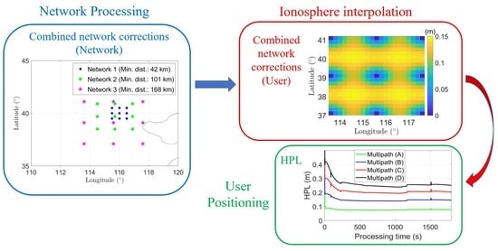
In the following subsections, the results of (i) network processing, (ii) user processing and (iii) HPLs are presented and discussed.

4.1. Network Processing

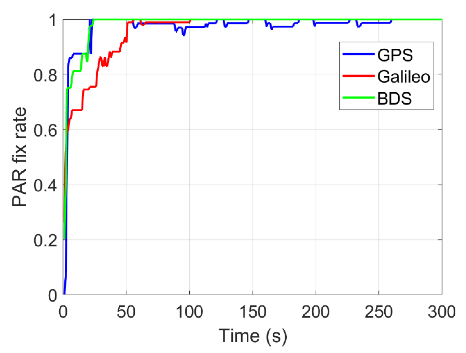
For each of the three networks mentioned before, the observations are simulated with the noise, hardware biases and the ZTDs as defined in Table 4. Figure 3 shows the fix rate of the PAR for the three constellations using Network 1. It can be observed that after about 5 min, FAR can be achieved for all three constellations. They remained resolved most of the time afterward.

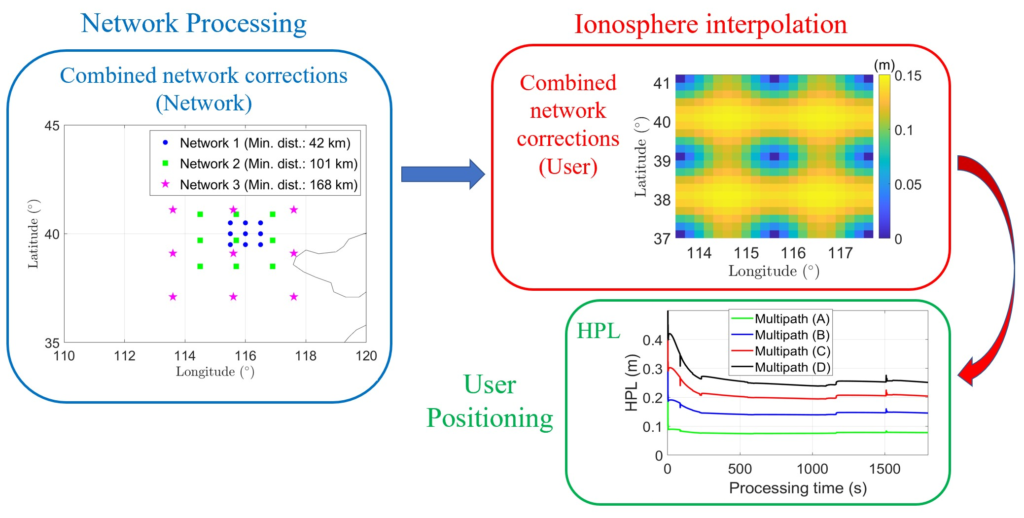
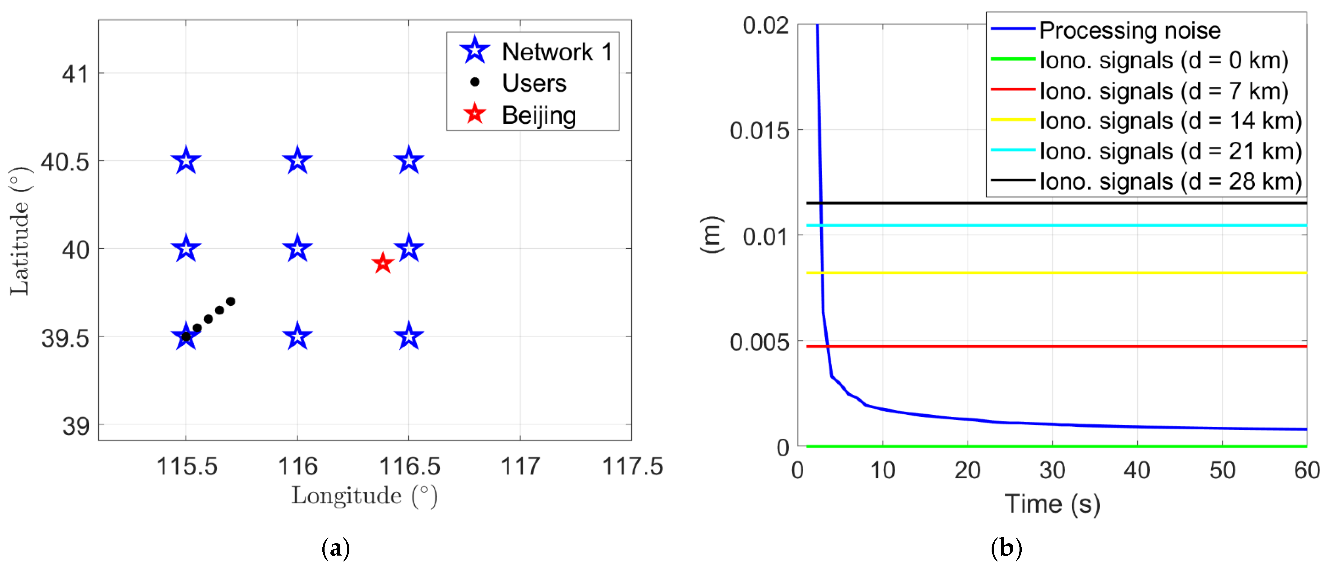
As mentioned in Section 2.2.2, the combined network corrections take an effective role at the between-satellite level in the user processing. Taking Network 1 as an example, the formal standard deviations of the between-satellite phase corrections on L1, for the satellite pair C26 and C29, are shown in Figure 4b with the user ionospheric delays predicted as explained in Section 2.2.1. The blue line corresponds to the errors induced only by the processing noise (the first part of the right side of Equation (14)), while the other colored lines correspond to the errors induced by the spatial correlation of the ionospheric signals (the second part of the right side of Equation (14)). The prediction matrices $F_{{\iota }_u}$ are also calculated differently considering only these two types of errors. The user is assumed to be located at different spots with an increasing inter-station distance to the bottom left network station, as shown in Figure 4a. Distance-dependent biases induced by ionospheric delays were proposed by [42,43]. Under a nominal ionospheric condition of 10 total electron content units (TECU), one may expect an ionospheric gradient of 1.5 mm/km for an elevation mask of 10 degrees. Assuming a Gaussian distribution of the ionospheric signals, the standard deviation of the differential ionospheric delays over 1 km baseline (${\sigma }_{{\iota }_{ij,1\mathrm{km}}}$), which corresponds to about 68% percentile of the differential ionospheric delays over 1 km, is set to 1.5 mm here for nominal conditions and was used in Figure 4b.

From Figure 4b it can be observed that with the PAR enabled, the standard deviation of the between-satellite network corrections induced by the processing noise (see the blue line) converges quickly to a very small value, i.e., below 1 mm; they become ignorable compared to that induced by the ionosphere interpolation. This implies that in case of limited bandwidth of the data transfer between the network and the user, the V-C matrix of the network corrections can be omitted after the convergence of the network solutions. In such a case, only the spatial correlation of the ionospheric signals will be considered for the ionosphere interpolation and for the V-C matrix of the network corrections.

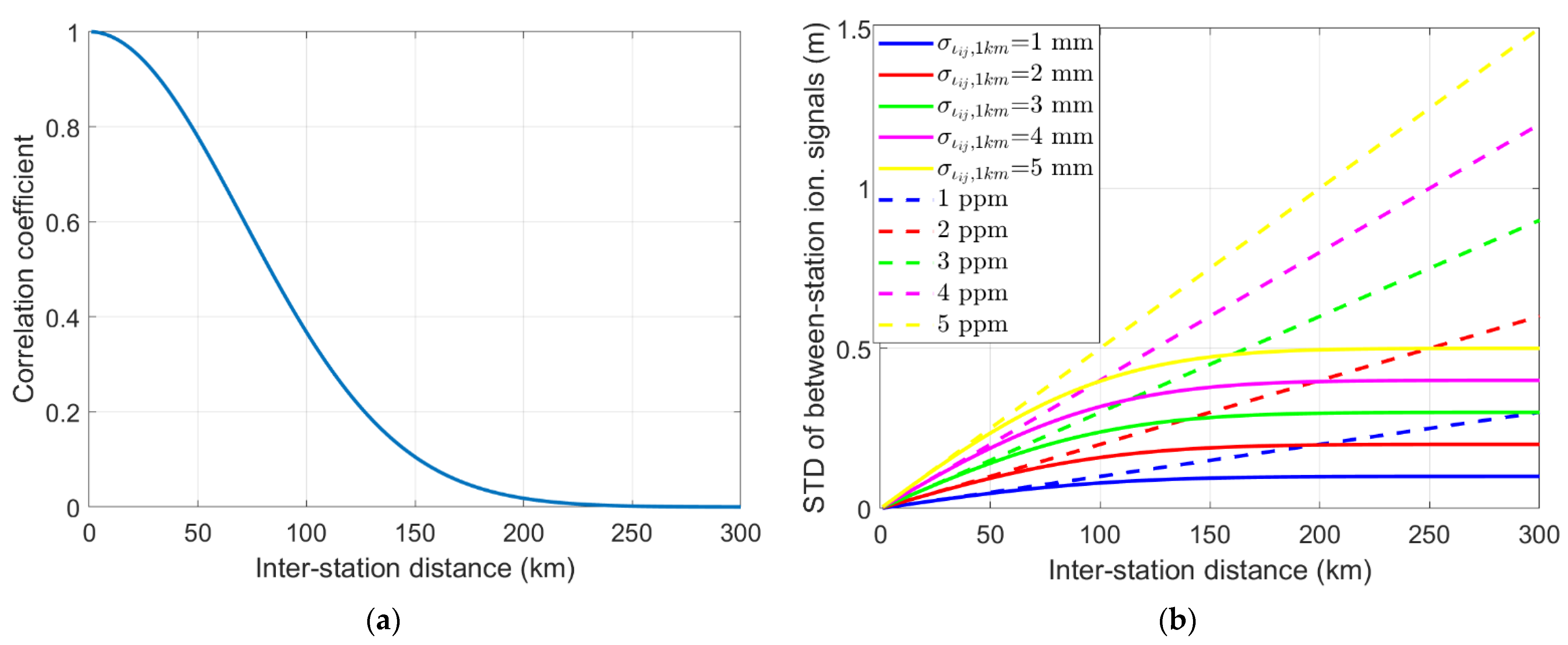
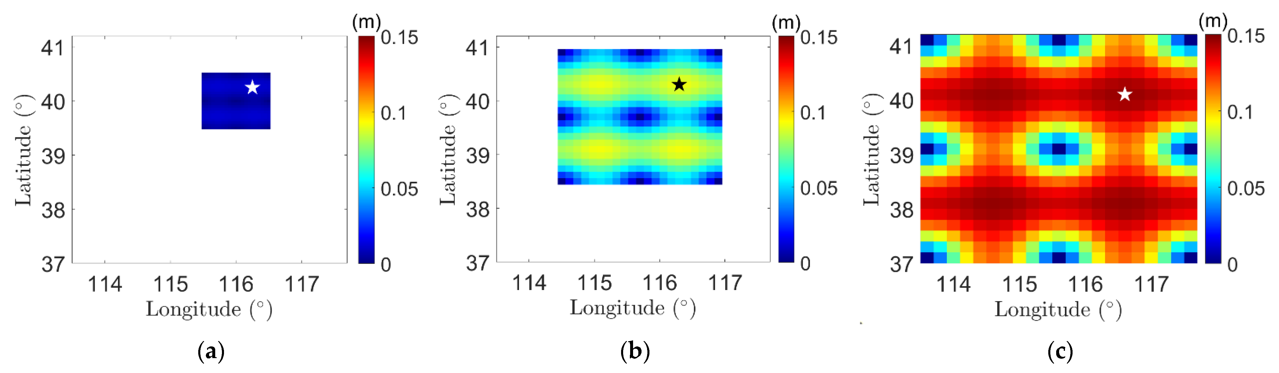
Figure 5 shows the colormaps of the precision of the between-satellite network corrections of C26 and C29 on L1 phase using Networks 1–3 after a convergence time of 60 s. Both the processing noise and spatial ionospheric signals are considered. The ${\sigma }_{{\iota }_{ij,1\mathrm{km}}}$ is set to 1.5 mm. It can be seen that the density of the network stations (see Figure 2) is an essential factor impacting the precision of the user ionosphere interpolation, and thus for that of the network corrections. Small inter-station distances of, e.g., about 40 km for Network 1 leads to a standard deviation of the between-satellite network corrections of around 1 cm on L1 phase, while the value increases to over 1 dm for an inter-station distance of about 170 km in Network 3. This would slow down the ambiguity resolution at the user side, and will be further explained in the next sub-section. For each network, one of the worst locations for the ionosphere interpolation (see the stars) is selected to evaluate the user positioning results and the IM. The distance from the star to the nearest network station amounts to about 35, 84 and 140 km, respectively, in the three networks.

4.2. User Processing

With the satellite clocks, satellite phase biases provided by the network and the ionospheric delays interpolated with the help of those of the network stations, the user can resolve the ambiguities and thus achieve high positioning precision. In this section, the observations of the worst-location users (see the stars in Figure 5) are simulated with the noise, the temporally linked ZTDs and hardware biases as defined in Table 4. Spatially correlated ionospheric signals are simulated for both the network stations and the user according to Equation (7). The interpolated ionospheric signals of the network stations are considered in the network corrections in addition to the processing noise.

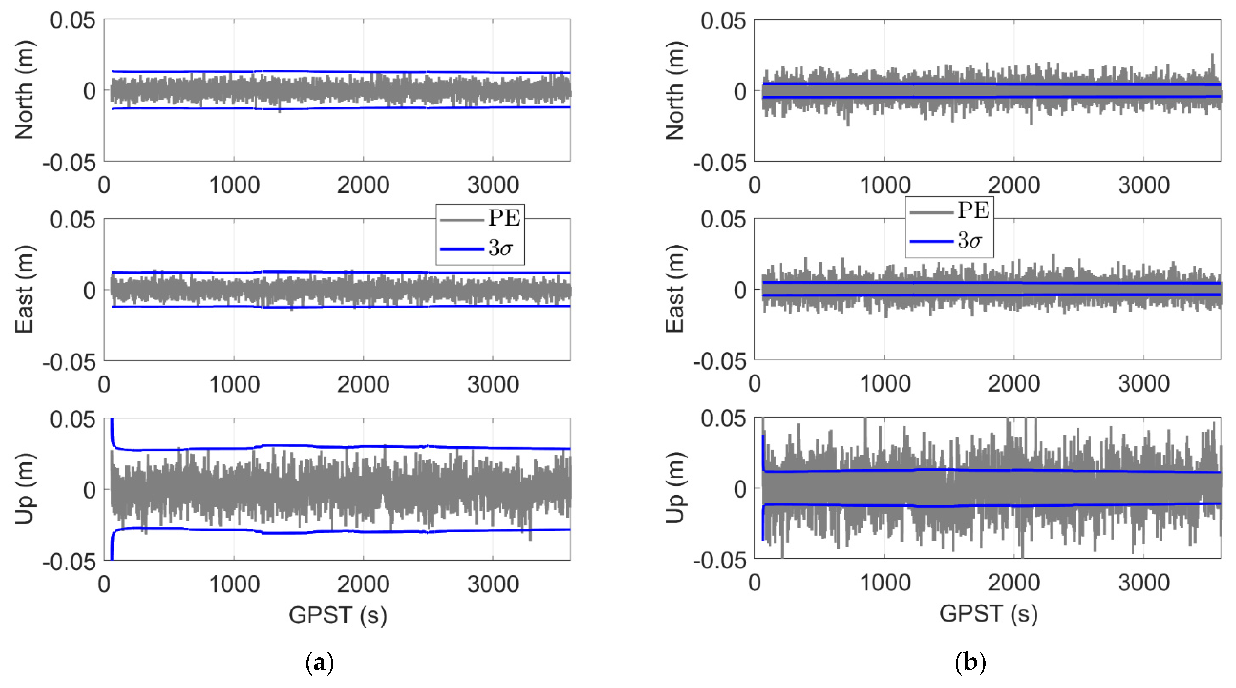
The blue lines in Figure 6 show three times the formal standard deviations of the user positions for Network 1, and the gray lines illustrate the corresponding PEs. The user processing starts 60 s after the network processing to allow for convergence of the network corrections, i.e., at 00:01:00 in GPST on 26 June 2021. FAR is achieved almost in the entire test period. The two panels of Figure 6 distinguish between two cases:

Option A: The V-C matrix of the network corrections, i.e., $Q_{\mathrm{c}}$ (see Equation (20)) is considered in the user processing.

Option B: The V-C matrix of the network corrections is not considered in the user processing.

From Figure 6a for Option A and Figure 6b for Option B it can be observed that applying the V-C matrix of the network corrections is not only helpful to reduce the PEs, but is also essential to obtain the correct formal standard deviations of the user positioning results. The blue lines in Figure 6b are shown to be too optimistic to bound about 99.7% of the PEs, which is expected for Gaussian noise. As shown in

Table 5. Statistics of the positioning results under different options for user at the worst location in Network 1.

Options	RMS of the PEs (m)			Percentage of the PEs Bounded by 3$\mathit{\sigma }$ (%)
	North	East	Up	North	East	Up
A	0.004	0.004	0.010	99.8	99.7	99.7
B	0.007	0.006	0.015	51.2	49.8	56.2

, while Option B could still deliver positioning results at an acceptable level, incorrect formal standard deviations of the user positioning results would directly lead to under-estimated PLs, which cannot bound the PEs under a given ${\mathrm{PMI}}_{\mathrm{H}}$ as expected.

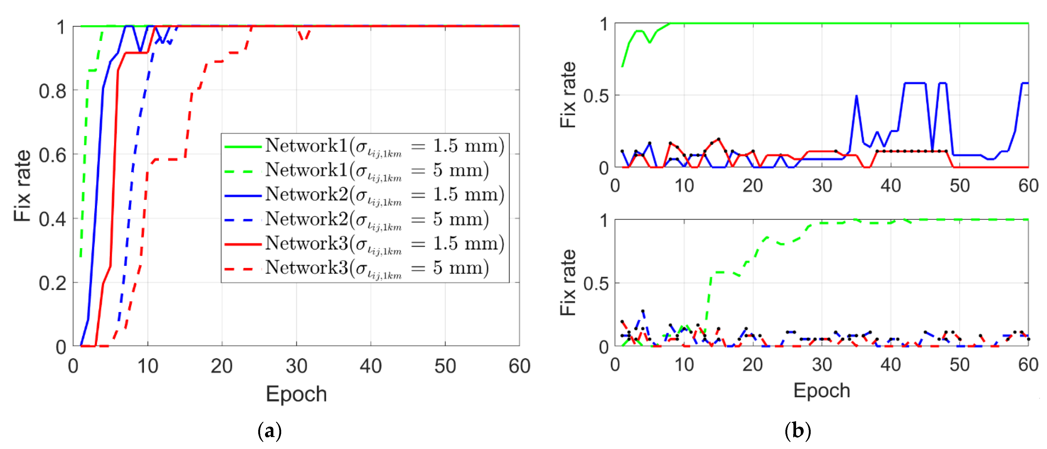
As discussed in the last subsection, the precision of the network corrections at the between-satellite level is mainly related to the user ionosphere interpolation. For different ionosphere activities and networks of different sizes, the user could experience different times to reach the FAR. Figure 7a shows the ambiguity fix rate for the three networks assuming a ${\sigma }_{{\iota }_{ij,1\mathrm{km}}}$ of 1.5 mm under nominal conditions, and 5 mm under more active ionosphere conditions. Compared to the instantaneous FAR for the small network under quiet ionospheric condition (see the solid green line in Figure 7a, the FAR is delayed by tens of epochs for Network 3 with a ${\sigma }_{{\iota }_{ij,1\mathrm{km}}}$ of 5 mm. When not considering the V-C matrix of the network corrections, for the purpose of visualization, the cases with a ${\sigma }_{{\iota }_{ij,1\mathrm{km}}}$ of 1.5 and 5 mm are illustrated in the top and bottom panels of Figure 7b, respectively. It can be seen that the FAR can still be achieved for the small network but over a longer period of time (see green lines), while for larger networks the results of the ambiguity resolution are shown to be bad. For Networks 2 (blue lines) and 3 (red lines), one does not only face a lower fix rate, but one also needs to deal with wrong fixing (see the black dots). Thus, correctly applying the V-C matrix of the network corrections is important for medium- to large-scale networks, or under active ionospheric conditions.

4.3. Horizontal Protection Level

For purpose of integrity at the user end, overbounding parameters are tested for a range of values as given in

Table 6. Overbounding parameters tested for integrity purpose.

Parameter	Explanation	Test Values
${\check{\sigma }}_{n0,\phi }$	Overbounding standard deviation of the zenith-referenced phase observations for network stations	0.005 m
${\check{\sigma }}_{n0,p}$	Overbounding standard deviation of the zenith-referenced code observations for network stations	0.5 m
${\check{\sigma }}_{u0,\phi }$	Overbounding standard deviation of the zenith-referenced phase observations for user	0.005–0.02 m
${\check{\sigma }}_{u0,p}$	Overbounding standard deviation of the zenith-referenced code observations for user	0.5–2 m
${\check{b}}_{u0,\phi }$	Overbounding bias of the zenith-referenced phase observations for user	0.01–0.04 cycles
${\check{b}}_{u0,p}$	Overbounding bias of the zenith-referenced code observations for user	0.2–0.8 m
${\check{\sigma }}_{{\iota }_{ij,1\mathrm{km}}}$	Overbounding standard deviation of between-station ionospheric signals at an inter-station distance of 1 km	5–20 mm
$\mathsf{\Delta }{\breve{\tau }}_r$, $\mathsf{\Delta }{\breve{\tau }}_u$	Overbounding spectral density of system noise for ZTDs	0.01 $\mathrm{m}/\sqrt{\mathrm{s}}$
${\mathrm{PMI}}_{\mathrm{H}}$	PMI in the horizontal direction	$2\times {10}^{-6}$–$2\times {10}^{-3}$

:

• The overbounding zenith-referenced standard deviations are of 5 mm and 0.5 m for the phase and code observations in the network processing, considering the fact that network stations are usually located at selected good measurement environments. One way to obtain the zenith-referenced overbounding parameters is given in [4] as an example at the between-receiver level, using ambiguity-fixed double-difference residuals for short baselines at the beginning.
• The overbounding standard deviation of the system noise for the temporally linked ZTDs is increased to 0.01 $\mathrm{m}/\sqrt{\mathrm{s}}$ to adapt to fast weather changes. The value could vary with the known weather, e.g., set to a looser value on rainy days.
• A range of overbounding standard deviations and biases are tested for the user observation noise/multipath, which are aimed to adapt to different complexities of the user multipath environment. They will be divided into different categories later in this section.
• For the ionosphere activities, [44] showed that the vertical overbounding standard deviation for the between-station ionospheric gradients are mostly below 4 mm/km in Switzerland over 15 years, with the maximum value of about 12 mm/km. Based on the modified single-layer model (SLM) [45], the slant ionospheric delay at an elevation angle of 10 degrees could be about 2.37 times that in the vertical direction. As such, the ${\breve{\sigma }}_{{\iota }_{ij,1\mathrm{km}}}$ is tested from 5 to 20 mm covering most non-extreme ionospheric conditions, while the extreme cases are supposed to be detected and excluded in the FDE process.

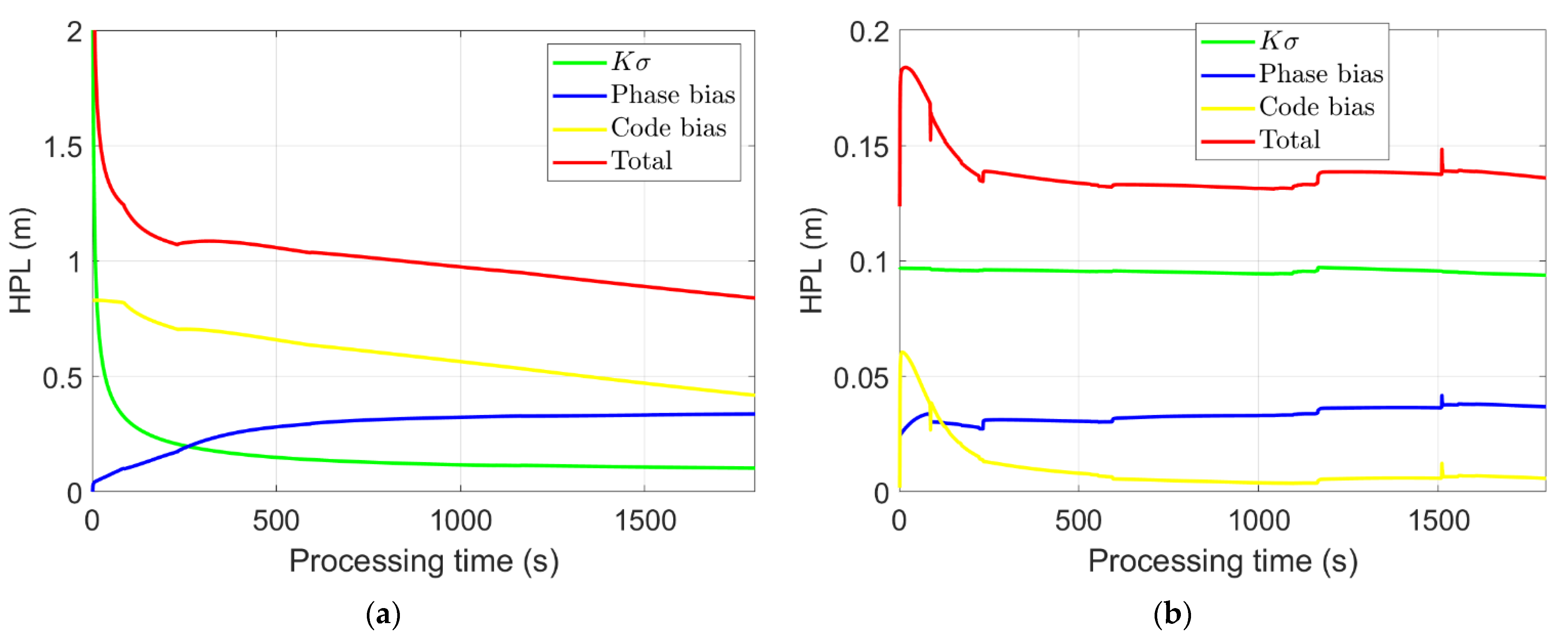
Figure 8 shows the contributions of different factors in computing the HPLs. In this example, assuming a nominal ionospheric condition, the worst-location user in Network 1 (see the star in Figure 5a) is used with ${\breve{\sigma }}_{{\iota }_{ij,1\mathrm{km}}}$ set to 10 mm. The overbounding standard deviations of the zenith-referenced phase and code noise/multipath (${\check{\sigma }}_{u0,\phi }$ and ${\check{\sigma }}_{u0,p}$) are set to 0.01 m and 1 m, respectively, and the corresponding overbounding biases (${\check{b}}_{u0,\phi }$ and ${\check{b}}_{u0,p}$) are set to 0.02 cycles and 0.4 m, respectively. For ionosphere interpolation, the ${\sigma }_{{\iota }_{ij,1\mathrm{km}}}$ for accuracy and continuity purpose is set to 1.5 mm. The ${\mathrm{PMI}}_{\mathrm{H}}$ is set to $2\times {10}^{-4}$. The green lines ($K\sigma$) represent the HPL contribution of the noise at the network and the user side (see the term $C^{-1}\left(\frac{{\mathrm{PMI}}_{\mathrm{H}}}{2\times 2}\right){\breve{\sigma }}_q\left(t_i\right)$ in Equation (35)), while the blue and yellow lines denote the HPL contributions of the biases originated from the phase and code multipath (see the term ${\breve{b}}_q\left(t_i\right)$ in Equation (35)). The red lines are the total HPLs.

From Figure 8 it can be observed that the float HPL is generally at meter level in the first half-hour, with the highest contribution coming from the code bias. With the PAR enabled, the FAR is achieved in almost the entire test period. The ambiguity-fixed HPL is at the dm-level, for which the diverse noise contribution plays a dominant role in our example. When the PAR is enabled, the phase bias has a higher contribution than the code bias due to the higher weighting of phase observations than that of code.

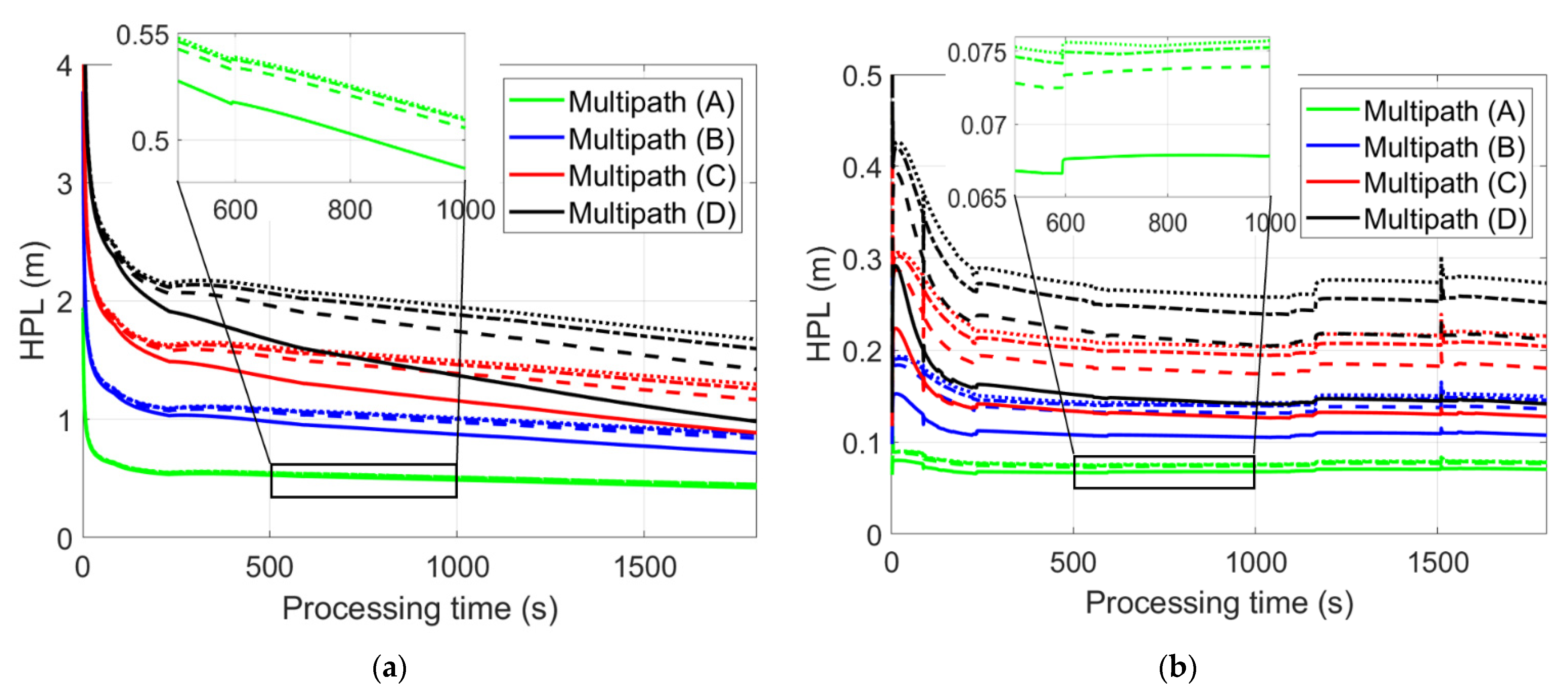
Different multipath and ionosphere conditions may lead to different HPL results. Here we categorize the user multipath environments into four categories based on different overbounding standard deviations (${\check{\sigma }}_{u0,\phi }$ and ${\check{\sigma }}_{u0,p}$) and biases (${\check{b}}_{u0,\phi }$ and ${\check{b}}_{u0,p}$) as shown in

Table 7. Overbounding parameters used for different categories of the multipath environments and ionosphere conditions.

Multipath Environment					Ionosphere Condition
Category	${\stackrel{\mathbf{ˇ}}{\mathit{\sigma }}}_{\mathit{u}\mathbf{0}\mathbf{,}\mathit{\phi }}$ (m)	${\stackrel{\mathbf{ˇ}}{\mathit{\sigma }}}_{\mathit{u}\mathbf{0}\mathbf{,}\mathit{p}}$ (m)	${\stackrel{\mathbf{ˇ}}{\mathit{b}}}_{\mathit{u}\mathbf{0}\mathbf{,}\mathit{\phi }}$ (cycle)	${\stackrel{\mathbf{ˇ}}{\mathit{b}}}_{\mathit{u}\mathbf{0}\mathbf{,}\mathit{p}}$ (m)	${\stackrel{\mathbf{ˇ}}{\mathit{\sigma }}}_{{\mathit{\iota }}_{\mathit{i}\mathit{j}\mathbf{,}\mathbf{1}\mathbf{k}\mathbf{m}}}$ (mm)	${\mathit{\sigma }}_{{\mathit{\iota }}_{\mathit{i}\mathit{j}\mathbf{,}\mathbf{1}\mathbf{k}\mathbf{m}}}$ (mm)
A	0.005	0.5	0.01	0.2	5	1.5
B	0.01	1	0.02	0.4	10	1.5
C	0.015	1.5	0.03	0.6	15	5
D	0.02	2	0.04	0.8	20	5

. Similarly, the ionosphere conditions are divided into four categories using different ${\check{\sigma }}_{{\iota }_{ij,1\mathrm{km}}}$. For ${\check{\sigma }}_{{\iota }_{ij,1\mathrm{km}}}\le$ 10 mm, the ${\sigma }_{{\iota }_{ij,1\mathrm{km}}}$ for accuracy and continuity purpose is set to 1.5 mm. For larger ${\check{\sigma }}_{{\iota }_{ij,1\mathrm{km}}}$, ${\sigma }_{{\iota }_{ij,1\mathrm{km}}}$ is set to 5 mm.

Figure 9 shows the HPLs of the worst-location user in Network 1 under different multipath environments and ionosphere conditions. The green lines of different types (multipath scenarios) are almost overwritten by each other and are zoomed in for better visualization for the processing time between 500 and 1000 s as examples. The solid, dashed, dashed-dotted and dotted lines represent the ionospheric conditions A, B, C and D, respectively. PAR is enabled in the right panel, and FAR is achieved most of the time. It can be observed that the multipath environments have significant influences on the HPLs, where increasing the complexity of the ionosphere condition further delays the convergence of the HPL, especially for complicated multipath environments. Figure 9 also shows that fixing ambiguities is essential to reduce the HPL from meters to decimeters.

Decreasing the ${\mathrm{PMI}}_{\mathrm{H}}$ would lead to a larger value in $C^{-1}\left(\frac{{\mathrm{PMI}}_{\mathrm{H}}}{2\times 2}\right)$ (see Equation (35)) and thus increase the HPL. As shown in Figure 10a, showing some examples for the multipath/ionosphere scenarios, the differences in ${\mathrm{PMI}}_{\mathrm{H}}$ (see the different line styles explained in the figure caption) does not lead to significant differences in the ambiguity-float HPLs due to the dominant behavior of the code biases. Again, the green lines of different types (multipath/ionosphere scenarios) are almost overwritten by each other and are zoomed in for better visualization for the processing time between 500 and 1000 s as examples. In the ambiguity-fixed scenario (Figure 10b), where the noise plays the dominant role, the differences caused by ${\mathrm{PMI}}_{\mathrm{H}}$ become more apparent, especially for complicated multipath/ionosphere conditions (D) with weak observation model and large ${\breve{\sigma }}_q$.

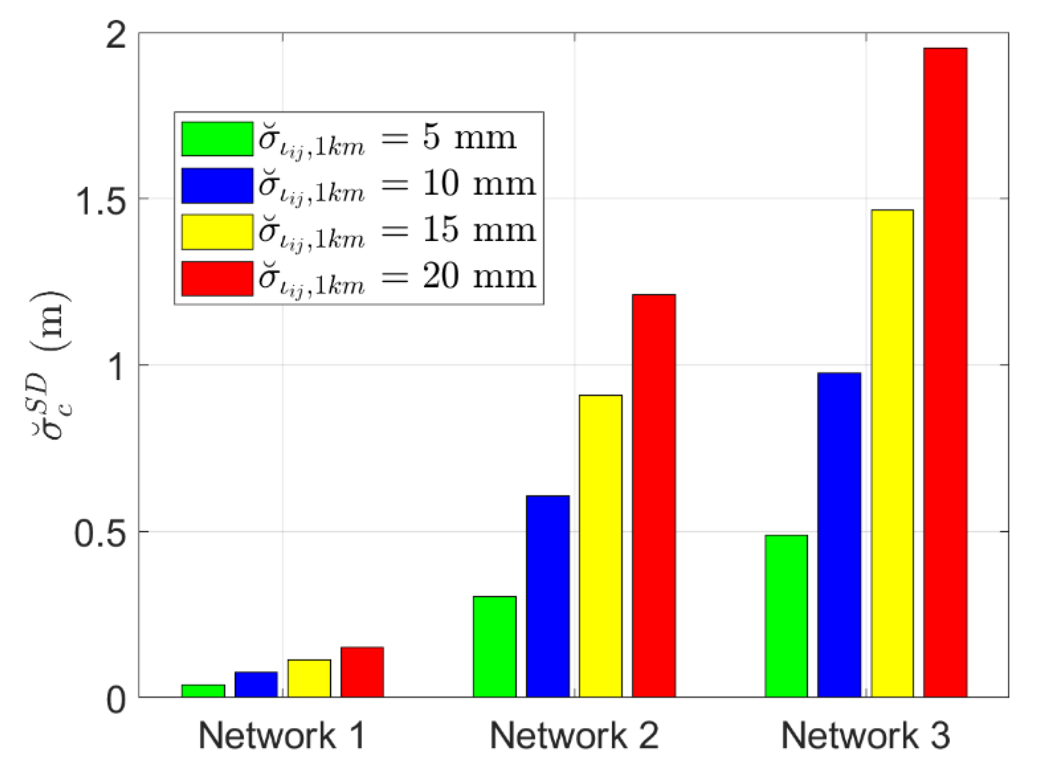
Under the same ${\check{\sigma }}_{{\iota }_{ij,1\mathrm{km}}}$, larger network size would lead to worse precision in the ionosphere interpolation. Figure 11 shows the overbounding standard deviations of the between-satellite network corrections (${\breve{\sigma }}_{\mathrm{c}}^{\mathrm{SD}}$) for satellite pair C26 and C29 for the worst-location users at the end of a half-hour session. It can be observed that the network size significantly impacts the ionosphere interpolation, where the overbounding standard deviations delivered by the small-scaled Network 1 under active ionosphere conditions are lower than those of Network 2 under quiet conditions. Sorted with the ${\breve{\sigma }}_{\mathrm{c}}^{\mathrm{SD}}$, the HPLs are plotted in Figure 12 for different multipath scenarios and ${\mathrm{PMI}}_{\mathrm{H}}$. In the ambiguity-float case, i.e., Figure 12a, the green lines of different types (multipath scenarios) are almost overwritten by each other and are zoomed in for better visualization for ${\breve{\sigma }}_{\mathrm{c}}^{\mathrm{SD}}$ from 0.5 to 1 m as examples. It can be seen that sharp increase in the HPLs exists at small values of ${\breve{\sigma }}_{\mathrm{c}}^{\mathrm{SD}}$, especially for complicated multipath environments. This indicates that in urban areas with high multipath, under nominal ionosphere condition, decreasing the network scale could be an efficient way in reducing the HPL. For all the tested multipath scenarios, the HPLs do not vary much when ${\breve{\sigma }}_{\mathrm{c}}^{\mathrm{SD}}$ exceeds 0.5 m. Further increasing ${\breve{\sigma }}_c^{\mathrm{SD}}$ mainly disturbs other parameters rather than the horizontal coordinates. This is especially obvious for the ambiguity-fixed scenario, while the float ambiguities disturbed by ${\breve{\sigma }}_{\mathrm{c}}^{\mathrm{SD}}$ still have influences on the horizontal coordinates.

Table 8. Time-to-convergence (TOC) to 1.5 m for ambiguity-float HPLs for multipath scenarios A–D. Under each multipath scenario, the TOC for ${\mathrm{PMI}}_{\mathrm{H}}$ of $2\times {10}^{-3},$ $2\times {10}^{-4}$, $2\times {10}^{-5}$ and $2\times {10}^{-6}$ are separated by “/”. “-” represents the case when convergence is not reached until 30 min.

${\stackrel{\mathbf{˘}}{\mathit{\sigma }}}_{\mathit{c}}^{\mathbf{S}\mathbf{D}}$ (m)	Network	${\stackrel{\mathbf{ˇ}}{\mathit{\sigma }}}_{{\mathit{\iota }}_{\mathit{i}\mathit{j}\mathbf{,}\mathbf{1}\mathbf{k}\mathbf{m}}}$ (mm)	TOC (s)
			Multipath A	Multipath B	Multipath C	Multipath D
0.04	1	5	2/2/3/3	16/22/29/36	183/221/306/356	712/765/809/846
0.08	1	10	2/2/3/4	17/23/31/38	495/573/675/754	1536/1602/1659/1710
0.11	1	15	2/2/3/4	17/24/32/40	723/846/943/1025	-/-/-/-
0.15	1	20	2/3/3/4	17/25/32/41	853/975/1077/1171	-/-/-/-
0.30	2	5	2/3/4/5	18/26/35/44	1018/1141/1233/1310	-/-/-/-
0.49	3	5	3/4/5/6	20/29/39/49	1124/1225/1310/1386	-/-/-/-
0.61	2	10	3/5/6/7	22/32/43/55	1050/1174/1259/1338	-/-/-/-
0.91	2	15	5/7/9/11	28/42/57/74	1069/1186/1273/1351	-/-/-/-
0.98	3	10	6/8/10/12	30/44/60/79	1153/1248/1332/1406	-/-/-/-
1.21	2	20	8/12/15/19	37/57/81/99	1118/1222/1307/1382	-/-/-/-
1.46	3	15	13/18/24/30	50/81/124/157	1225/1317/1395/1464	-/-/-/-
1.95	3	20	29/42/57/72	170/215/339/383	1330/1413/1484/1545	-/-/-/-

and

Table 9. Time to convergence (TOC) to 0.3 m for ambiguity-fixed HPLs for multipath scenarios A–D. Under each multipath scenario, the TOC for ${\mathrm{PMI}}_{\mathrm{H}}$ of $2\times {10}^{-3},$ $2\times {10}^{-4}$, $2\times {10}^{-5}$ and $2\times {10}^{-6}$ are separated by “/”. “-” represents the case when convergence is not reached until 30 min.

${\stackrel{\mathbf{˘}}{\mathit{\sigma }}}_{\mathit{c}}^{\mathbf{S}\mathbf{D}}$ (m)	Network	${\stackrel{\mathbf{ˇ}}{\mathit{\sigma }}}_{{\mathit{\iota }}_{\mathit{i}\mathit{j}\mathbf{,}\mathbf{1}\mathbf{k}\mathbf{m}}}$ (mm)	TOC (s)
			Multipath A	Multipath B	Multipath C	Multipath D
0.04	1	5	1/1/1/1	1/1/1/1	1/1/1/1	1/1/22/32
0.08	1	10	1/1/1/1	1/1/1/1	1/1/30/52	68/87/104/130
0.11	1	15	2/2/2/2	2/2/2/2	4/32/68/91	106/141/185/517
0.15	1	20	2/2/2/2	2/2/2/2	2/50/87/117	138/189/463/-
0.30	2	5	4/4/4/4	4/4/4/4	5/76/123/170	205/376/-/-
0.49	3	5	6/6/6/6	6/6/6/6	6/74/130/185	220/466/-/-
0.61	2	10	4/4/4/4	4/4/4/4	5/76/127/179	222/484/-/-
0.91	2	15	9/9/9/9	9/9/9/9	9/71/122/174	222/506/-/-
0.98	3	10	6/6/6/6	6/6/6/6	6/66/123/177	220/506/-/-
1.21	2	20	9/9/9/9	9/9/9/9	9/67/117/167	222/506/-/-
1.46	3	15	10/10/10/10	16/16/16/16	16/60/114/164	220/498/-/-
1.95	3	20	10/10/10/16	16/16/16/16	16/56/147/164	215/484/-/-

list the time-to-convergence (TOC) to 1.5 m for the ambiguity-float HPLs and to 0.3 m for the ambiguity-fixed HPLs. TOC is defined as the processing time needed to reach a certain threshold of the HPL and maintain it below this threshold for at least 60 s. From Table 8 and Table 9, it can be observed that under the same ${\breve{\sigma }}_c^{\mathrm{SD}},$ the multipath environment generally has the largest influence on the TOC. With the increasing complexity of the multipath environment, the impact of the ${\breve{\sigma }}_{\mathrm{c}}^{\mathrm{SD}}$ on the HPLs increases. This shows that to quickly reach and thereafter maintain a low HPL in complicated multipath environments, it is essential to shrink the network size to keep a low ${\breve{\sigma }}_c^{\mathrm{SD}}$. In simple multipath environments (like Multipath scenario A), a small network scale would be helpful to accelerate the ambiguity resolution, as mentioned in Section 4.2. With the ambiguities fixed, the HPLs do not appear to differ much for different ${\breve{\sigma }}_{\mathrm{c}}^{\mathrm{SD}}$ (see also Figure 12b). In general, in nominal multipath environments (A/B), the ambiguity-float HPLs could converge to 1.5 m for Networks 1 and 2 under quiet to medium ionosphere activities (${\check{\sigma }}_{{\iota }_{ij,1\mathrm{km}}}\le 10$ mm) within or around 50 epochs for all the tested ${\mathrm{PMI}}_{\mathrm{H}}$. In the ambiguity-fixed case and under multipath scenarios A/B, the HPLs could converge to 0.3 m for Networks 1 and 2 even under active ionosphere conditions within ten epochs. Recall that for ambiguity resolution and ionosphere interpolation, the ${\sigma }_{{\iota }_{ij,1\mathrm{km}}}$ for accuracy and continuity purposes is used, i.e., 1.5 mm for ${\check{\sigma }}_{{\iota }_{ij,1\mathrm{km}}}\le 10$ mm, and 5 mm for 10 mm $<{\check{\sigma }}_{{\iota }_{ij,1\mathrm{km}}}\le 20$ mm (see Table 7).

5. Conclusions

This contribution proposes a general method for IM of the PPP-RTK horizontal positioning from networks of different scales. Using the ionosphere-weighted model, the V-C matrix of the interpolated user ionospheric delays as well as other combined network corrections is considered for accuracy and continuity purposes in the user positioning, and for its integrity monitoring purpose in the user IM. It was found that considering the V-C matrix of the network corrections is essential for quick and successful ambiguity fixing, and for computation of correct PLs that bound the PEs as expected.

Using GPS L1 and L5 and Galileo/BDS equivalent frequencies with a sampling interval of 1 s, it was found that the HPLs and their convergence are closely dependent on the user multipath environment and the overbounding standard deviations of the network corrections at the between-satellite level, where the latter term is again closely related to the ionosphere interpolation, i.e., the ionosphere activity and the network scale. For small- to mid-scaled networks, under nominal multipath environments and for a ${\mathrm{PMI}}_{\mathrm{H}}$ down to $2\times {10}^{-6}$, the ambiguity-float HPLs can converge to 1.5 m within (or around) 50 epochs under quiet to medium ionosphere activities. Under the same multipath conditions and for the same network scales, with the PAR enabled, the HPLs can converge to 0.3 m within 10 epochs even under active ionosphere activities, provided that the V-C matrix of the network corrections are correctly considered during the user processing.

There are a few open issues to be studied in future works:

• The overbounding bias caused by multipath propagates within the filter at the user side (see Equation (37)). The direct approach of correctly considering the time-propagated biases of each epoch requires the user to save the projection matrices (from the observation- to the position-domain) from each starting epoch to the previous epoch, and thereafter perform matrix multiplications for all these starting epochs to build those for the current epoch. This is memory-consuming for long sessions. Methods to simplify this procedure need to be investigated.
• In this study, the spatial correlation of the ionospheric signals is calculated using a Gaussian function, with the applicable distance $l_0$ set to 100 km. The model is only used as an example for demonstration purposes. For a specific network, the spatial correlation is suggested to be studied empirically.
• This study does not protect against wrong ambiguity fixing. As such, in addition to the ratio test, the resolved ambiguities are suggested to be validated using other methods that do not strongly related to the V-C matrix of the float ambiguities, which could be influenced by model deficiencies.