Stability of CubeSat Clocks and Their Impacts on GNSS Radio Occultation

Abstract

Global Navigation Satellite Systems’ radio occultation (GNSS-RO) provides the upper troposphere-lower stratosphere (UTLS) vertical atmospheric profiles that are complementing radiosonde and reanalysis data. Such data are employed in the numerical weather prediction (NWP) models used to forecast global weather as well as in climate change studies. Typically, GNSS-RO operates by remotely sensing the bending angles of an occulting GNSS signal measured by larger low Earth orbit (LEO) satellites. However, these satellites are faced with complexities in their design and costs. CubeSats, on the other hand, are emerging small and cheap satellites; the low prices of building them and the advancements in their components make them favorable for the GNSS-RO. In order to be compatible with GNSS-RO requirements, the clocks of the onboard receivers that are estimated through the precise orbit determination (POD) should have short-term stabilities. This is essential to correctly time tag the excess phase observations used in the derivation of the GNSS-RO UTLS atmospheric profiles. In this study, the stabilities of estimated clocks of a set of CubeSats launched for GNSS-RO in the Spire Global constellation are rigorously analysed and evaluated in comparison to the ultra-stable oscillators (USOs) onboard the Constellation Observing System for Meteorology, Ionosphere, and Climate (COSMIC-2) satellites. Methods for improving their clock stabilities are proposed and tested. The results (i) show improvement of the estimated clocks at the level of several microseconds, which increases their short-term stabilities, (ii) indicate that the quality of the frequency oscillator plays a dominant role in CubeSats’ clock instabilities, and (iii) show that CubeSats’ derived UTLS (i.e., tropopause) atmospheric profiles are comparable to those of COSMIC-2 products and in situ radiosonde observations, which provided external validation products. Different comparisons confirm that CubeSats, even those with unstable onboard clocks, provide high-quality RO profiles, comparable to those of COSMIC-2. The proposed remedies in POD and the advancements of the COTS components, such as chip-scale atomic clocks and better onboard processing units, also present a brighter future for real-time applications that require precise orbits and stable clocks.

1. Introduction

Global Navigation Satellite Systems’ Radio Occultation (GNSS-RO) is an atmospheric remote sensing/atmospheric sounding technique currently being employed to complement the radiosonde [1] and reanalysis [2,3] products in order to improve the derived upper tropopause-lower stratosphere (UTLS) atmospheric profiles used in numerical weather prediction (NWP) models that generate global weather forecasting [4], as well as climate change studies [5,6]. GNSS-RO operates in such a way that the precise phase observations of a rising or setting GNSS satellite, which increase while passing through the atmospheric layers, are collected by the receivers onboard low Earth orbit (LEO) satellites. The measured phase delays (also called excess phases) are used to derive bending angles, which form the key observable used to retrieve the atmospheric profiles of temperature and pressure needed for NWP models as well as climate change studies (see, e.g., [7,8]). GNSS-RO theory, including the inversion of the phase delays to the atmospheric refractivity using Abel transformation, is well documented in different literature, e.g., [7,8,9,10,11,12,13].

Different larger LEO satellites, such as Gravity Recovery and Climate Experiment (GRACE [14]), Meteorological Operational (MetOp [15]), and Constellation Observing System for Meteorology, Ionosphere, and Climate (COSMIC-1 [14], and COSMIC-2 [16]), are equipped with the RO antennas suited for the GNSS-RO [17]. However, these satellites are utilised with the high-grade components in their buses and payloads, which increase their complexity, budget, and the time required for building and launching. In terms of costs, for example, COSMIC-1 and -2 required more than USD 100 and USD 460 million, respectively, to be completed [18]. As opposed to the larger LEO satellites above, low-cost CubeSats such as 3U CanX-2 [19] and 3U ARMADILLO [20] are currently being tested for GNSS-RO applications. CubeSats in general are small low-cost satellites with limited power budgets that are built from the commercial off-the-shelf (COTS) components in 10 × 10 × 10 cm³ units (1U). A 3U CubeSat can cost USD 20 K–USD 200 K depending on the onboard payload. The launch cost could be less than USD 40 K, which can be significantly reduced for mass launches in a constellation since several CubeSats will have a ride-share. The complexity and required budget, as well as the building time, of CubeSats are much less than those of larger LEO satellites, where these factors may even prevent the continuation of larger LEO missions, as evidenced in the second phase of COSMIC-2 that was cancelled due to funding problems [21]. Moreover, the technological advancements in the COTS components and the possibility of launching them in a constellation make them comparable to the larger LEO satellites in terms of their applicability in a wide range of space and earth science applications.

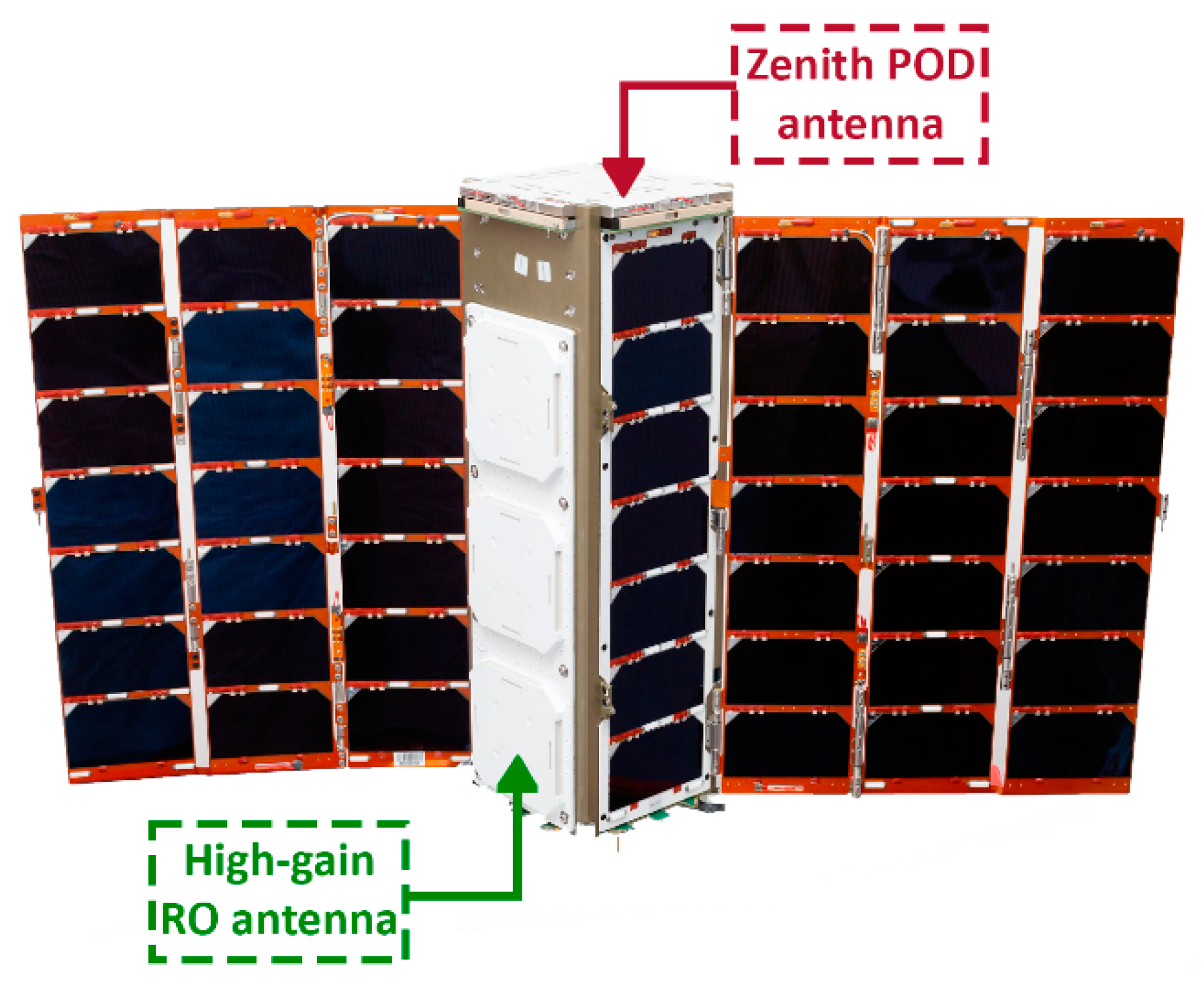
The mega constellation of CubeSats launched by Spire Global Inc. [https://spire.com accessed on 12 January 2022] is an example of CubeSats’ constellation that provides different services such as global weather monitoring using the GNSS-RO procedure, maritime domain awareness, and automatic dependent surveillance-broadcast. This constellation consists of more than 145 3U CubeSats (10 × 10 × 30 cm³) equipped mostly with STRATOS GNSS receivers that collect 50-Hz dual-frequency GNSS-RO signals. These signals and those that are collected by the zenith antenna mounted for the precise orbit determination (POD) are processed in the analysis center to provide daily globally distributed and high-quality atmospheric vertical profiles that bring substantial benefits to the performance of the NWP models [22].

To achieve accurate UTLS atmospheric profiles, however, the orbital accuracy of LEO satellites used for GNSS-RO should be at several centimeters level, and the velocity components, mainly along-track direction, should be better than 0.2 mm/s [23]. 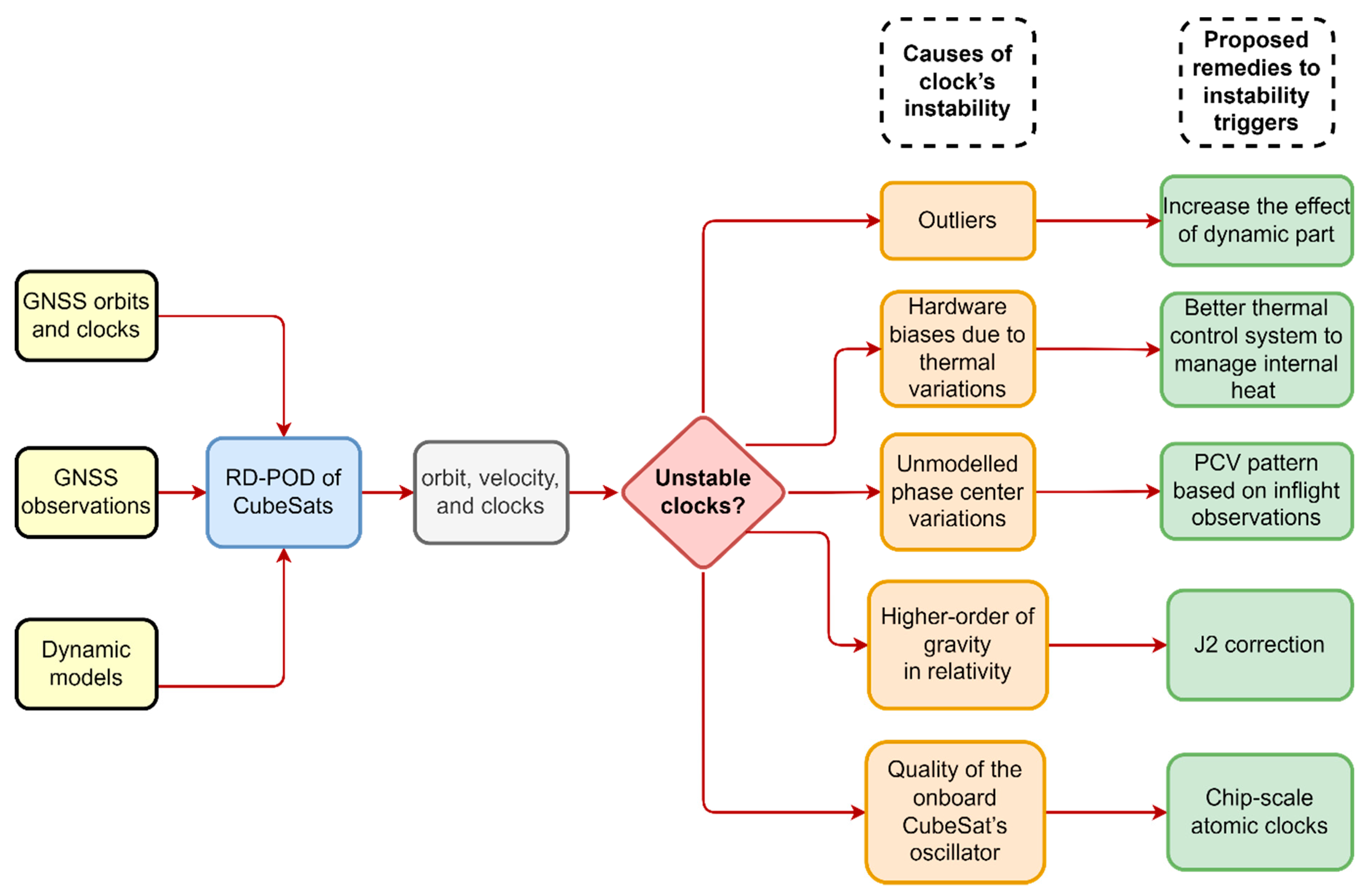The orbital precisions and accuracies of the Spire CubeSats have already been estimated using the reduced-dynamic POD (RD-POD) and internally validated in [24] and found to be at an acceptable range for the GNSS-RO application. Besides the orbital parameters, the accuracy of the estimated clocks and their stabilities are essential for GNSS-RO since the high-rate observations, e.g., at 50 Hz sample intervals, should be precisely time-tagged based on the estimated clock offsets. As such, any error or instability in these clocks affects the measured phase observations and subsequently the derived GNSS-RO atmospheric profiles.

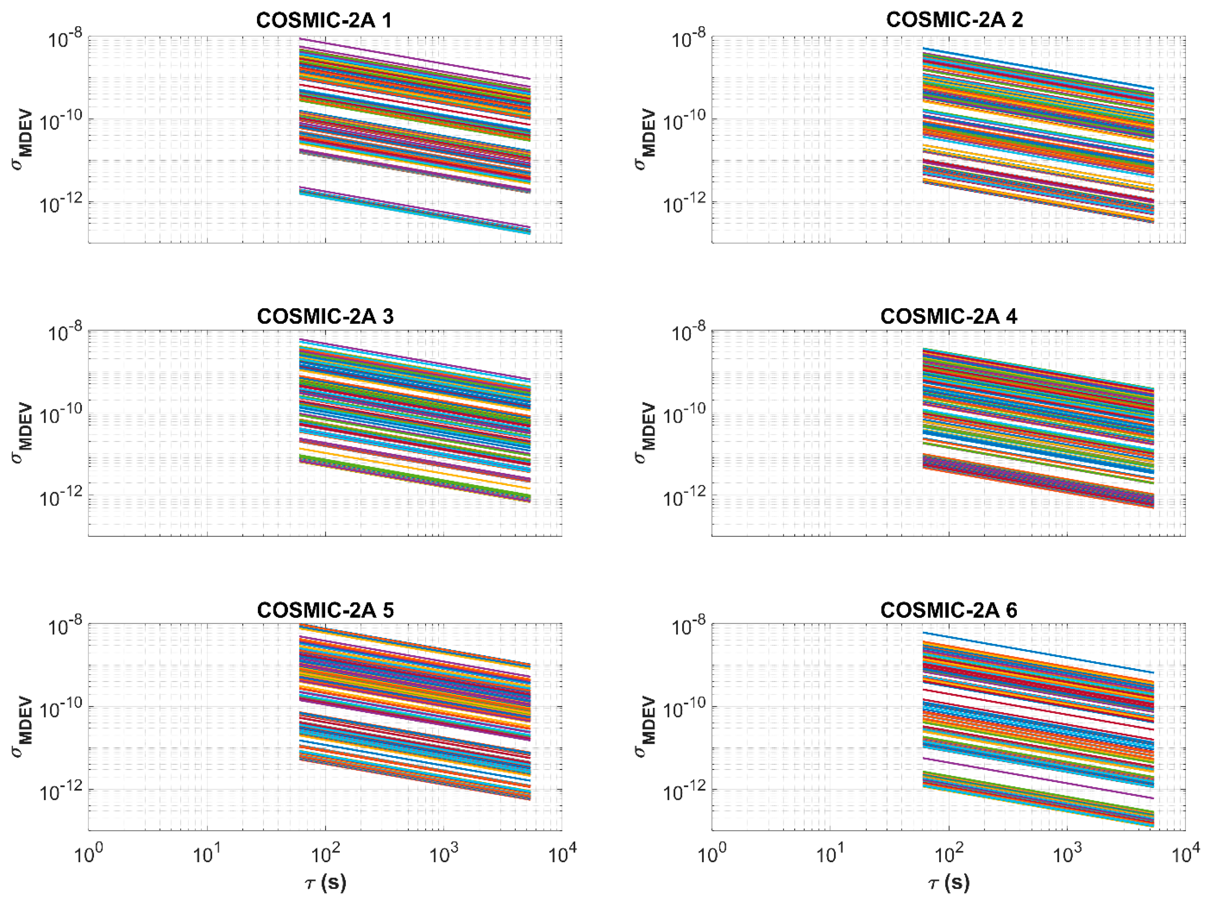
The accuracy of the estimated clocks and their stabilities are influenced by the quality of the oscillators and the remaining GNSS errors in the RD-POD models [25]. Larger LEO satellites (e.g., GRACE and COSMIC-2) are generally equipped with highly accurate oscillators that provide high stabilities at the ${10}^{-12}$ to ${10}^{-14}$ level [26,27]. However, this level of stability can be degraded by any unmodelled errors in the RD-POD procedure or the GNSS data quality. For example, the reduction in the clock stabilities to the ${10}^{-9}$ to ${10}^{-11}$ level, which is observed for COSMIC satellites, has been related to the quality of the GPS observations due to the inclined POD antenna orientation and its field of view, the accuracy of the attitude control systems, and the quality and the type of the onboard GPS receiver [26]. In addition, some periodic variations due to the GPS orbital period have been found in the GRACE clock analysis and proposed to be considered in the clock modelling [28]. For CubeSats, however, besides the general studies that show the CubeSats’ evolution (e.g., [29]) and their capabilities in the earth science applications (e.g., [30]), most studies have concentrated on evaluating the stabilities of the onboard CubeSats’ oscillators and developing compatible atomic clocks based on CubeSats’ limitations. For example, Warren et al. [31] analysed the developed atomic clocks based on optical pumping for the CubeSats while Rybak et al. [32] simulated the performance of the chip-scale atomic clocks for the navigation of a CubeSat in lunar orbit. To the best of the authors’ knowledge, no literature exists on the assessment and evaluation of CubeSats’ clock stabilities due to un-modelled errors in the POD procedure and their propagated impacts on the determined GNSS-RO profiles.

This study aims at assessing and evaluating the CubeSats’ clock stabilities and their possible impacts on the derived UTLS atmospheric products. The specific objectives of the study are (i) assessing CubeSats’ clock stabilities resulting from un-modelled errors during the RD-POD procedure and evaluating possible remedies, and (ii) analysing the derived GNSS-RO profiles from unstable CubeSats’ clocks in comparison to COSMIC-2. Section 2 starts by presenting the RD-POD procedure and the excess phase derivation before assessing CubeSats’ clock instabilities emanating from GNSS observational quality, hardware biases, un-modelled phase center variations, and relativistic effects. To have a better understanding of the ranges of the errors in the RD-POD compared to the quality of oscillators and their influences on the CubeSats’ clocks, the estimated clocks are compared to those of COSMIC-2 that have USOs. These are also analysed for the first time from the stability of receiver clocks’ point of view. Possible remedies in the RD-POD procedure to improve the accuracy of the estimated clocks are evaluated and discussed in addition to addressing the practical solutions for the unstable CubeSats’ clocks in GNSS-RO. To evaluate the CubeSats’ GNSS-RO atmospheric profiles derived from the excess phase observations while the CubeSats’ clock errors are removed using the complex solutions, they are compared in Section 3 to those of COSMIC-2 profiles and in situ radiosonde observations, which provide a completely independent data source for validation. Section 4 summarises and concludes the study.

2. CubeSats’ Clock Analysis

2.1. POD and Excess Phase Derivation

GNSS RO’s excess phase is derived from the phase observation ($\Delta {\Phi }_{r,j}^s$) between the GNSS satellite $s$ and the CubeSat’s onboard receiver $r$ for the frequency $j$ through

$$\Delta {\Phi }_{r,j}^s={\rho }_r^s+c\left(d{t}_r-d{t}^s\right)-d{I}_{r,j}^s+d{A}_r^s+{ϵ}_j$$

(1)

where ${\rho }_r^s$ is the true range between the GNSS satellite and the CubeSat, and $c$ is the speed of light that transforms the satellite and receiver clock offsets ($d{t}^s$ and $d{t}_r$) into computed ranges. The phase delays due to the ionosphere and the neutral atmosphere are indicated by $d{I}_{r,j}^s$ and $d{A}_r^s$, respectively, while ${ϵ}_j$ denotes the unmodelled observation noises. The phase observation in Equation (1) ignores the phase ambiguities since the time derivatives of the phase observations are the actual parameters of interest in GNSS-RO [33]. The wind-up effect, relativity term, phase center offsets (PCO) and variations (PCV), and clock hardware biases are first applied in Equation (1). Besides the available precise orbits and clocks of the GNSS satellites from network processing, precise orbits and the onboard receiver clock offsets of CubeSat are also required in order to derive the excess phase in Equation (1). From the excess phase, bending angles are then derived provided that the along-track component of the velocity vectors and the excess Doppler shifts are available [10].

The satellite’s state vector including the orbital and velocity components, as well as the onboard clock offsets, are estimated using the RD-POD method that is mainly based on the precise phase observations collected by the zenith POD antenna, which takes advantage of the available extensive dynamic models, as well as estimating some pre-defined stochastic accelerations to compensate for the dynamic model deficiencies [34]. The observations used in the RD-POD are subjected to the following pre-processing steps for outlier detection:

-

Identification of large magnitude outliers through single-differencing between GNSS satellites, and then comparing them with low-degree polynomials in order to eliminate them from the POD processing.

-

Detection of cycle slips by forming the ionosphere-free linear combinations and checking the differences between two consecutive epochs.

-

Detection of millisecond clock jumps from which new ambiguities are introduced.

In the above pre-processing steps, the a priori coarse orbits generated from code observations are used whenever CubeSat’s coordinates are required. However, these orbits are not good enough for reliable data screening. Therefore, the pre-processing steps are carried out iteratively (see [34] for more details).

Table 1. POD processing models and parameters.

Item	Description
Dynamic models	Gravity field: Earth Gravitational Model (EGM 2008) [38]
	Tidal corrections: Updated Finite Element Solution tidal model (FES2004) [39]
	Relativity: International Earth rotation and Reference systems Service (IERS 2010) [40]
	Planets ephemeris: Jet Propulsion Laboratory Development Ephemeris (JPL DE405) [41]
Observation model	Dual-frequency GPS Ionosphere-Free (1 Hz)
	Removing the required GNSS satellites using the cylindrical shadow model [42]
	A priori code standard deviation of 0.1 m, a priori phase standard deviation of 1 mm (Zenith, L1)
	Satellite attitude information: Obtained as quaternions
	PCO and PCV for GNSS satellites: igs14.atx [43]
	PCO and PCV for CubeSats: LEMUR_ant-1931.atx (Provided by Spire Global Inc.)
	GNSS orbits and clocks: Center for Orbit Determination in Europe (CODE) final products [44]
	GNSS satellite phase biases: CODE P1C1 and P2C2 Differential Code Biases (DCB) are applied to be consistent with the precise ephemeris
Stochastic accelerations	Velocity changes (pulses) at certain epochs at every 15 min
	Piece-wise constant accelerations at 6 min intervals

provides the model and parameters that are used to solve the following least-squares problem for the CubeSats’ RD-POD procedure [35]:

$$E\left(\Delta {\Phi }_{r,IF}^s\right)=\left[A_o,A_d,A_a\right]{\left[X_o,X_d,X_a\right]}^T+cd{t}_r+{\lambda }_{IF}{N}_{IF}$$

(2)

where $E$ is the expectation operator, $\Delta {\Phi }_{r,IF}^s$ is the linearised ionospheric-free phase observations, and $A_o$, $A_d$, and $A_a$ are the design matrices containing the required partial derivatives of the observations and dynamic models with respect to the orbital components, dynamic parameters, and stochastic accelerations, respectively. The unknown $X_o$ vector includes the orbit and velocity elements. The coefficients related to the dynamic models and the stochastic accelerations are combined into the $X_d$ and $X_a$ matrices, respectively. The ionosphere-free (IF) wavelength (${\lambda }_{IF}$) transforms the IF phase ambiguities ($N_{IF}$) into computed ranges. The partial derivatives in Equation (2) are derived through the numerical integration of the variational equation [34,36]. The unknown parameters are generally derived using the so-called pre-elimination and back-substitution method [37].

2.2. Assessment of the CubeSats’ Clock Instabilities

GNSS and CubeSats’ clock offsets should be stable enough to be interpolated at the 50 Hz time tags of the phase observations in order to derive the excess phase observation from Equation (1). On the one hand, all GNSS satellites are equipped with high-grade atomic clocks, where their clock offsets are estimated through rigorous network processing [45]. The available GNSS precise clocks are, therefore, stable enough to be interpolated using polynomials to the high-rate observation time tags [46,47,48]. On the other hand, CubeSats’ clock stabilities are estimated through the RD-POD processing, and depend on the GNSS observation noises, near field multipath due to the CubeSat’s structure, the accuracy of GNSS orbits and clocks used in the RD-POD processing, deficiencies of the dynamic models regarding the non-gravitational forces, unmodelled hardware biases, and the quality of the oscillators [25]. Due to these factors, the modified Allan deviation ($MDEV$) with the averaging time ($\tau$) [49] is used to analyse the stability of the clock errors:

$$MDEV\left(\tau \right)=\sqrt{\frac{1}{2m^2{\tau }^2\left(n-3m+1\right)}{\displaystyle \sum }_{k=1}^{n-3m+1}{\left({\displaystyle \sum }_{k=i}^{k+m-1}\left(d{t}_{r,i+2m}-2d{t}_{r,i+m}+d{t}_{r,i}\right)\right)}^2}$$

(3)

where $n$ is the number of clock samples, $m$ is the averaging factor to compute $\tau$ from the sampling interval $t_0$ as $\tau =m{t}_0$, and $d{t}_r$ is the estimated clock offsets from the RD-POD processing. In the analysis undertaken in this study, the clock offsets of 17 CubeSats from the Spire Global constellation are estimated through a comprehensive RD-POD procedure and their stabilities are computed from Equation (3) for a period of one month (16 December 2020 to 15 January 2021). A list of the CubeSats analysed in this study and their specifications are presented in

Table 2. Specifications of seventeen CubeSats employed in this study. SSO: Sun-Synchronous Orbit, LTAN: Local Time of Ascending Node, LTDN: Local Time of Descending Node (provided by Spire Global Inc.).

ID	CubeSat’s Name	COSPAR ID	Altitude (km)	Orbit Type	Mass Size
099	LEMUR-2-JOHANLORAN	2019-018G	505	SSO (LTAN 09:30)	~5 kg 0.1 × 0.1 × 0.3 m3 (3U CubeSat)
100	LEMUR-2-BEAUDACIOUS	2019-018H
101	LEMUR-2-ELHAM	2019-018J
102	LEMUR-2-VICTOR-ANDREW	2019-018K
103	LEMUR-2-WANLI	2019-038S	530	SSO (LTAN 15:05)
104	LEMUR-2-LILLYJO	2019-038L
106	LEMUR-2-EJATTA	2019-038Z
107	LEMUR-2-MORAG	2019-038T
108	LEMUR-2-GREGROBINSON	2019-038AB
115	LEMUR-2-JPGSQUARED	2019-089D	550	Orbit inclination: 37°
116	LEMUR-2-ETHANOAKES	2020-061AC	540	SSO (LTDN 10:30)
117	LEMUR-2-THEODOSIA	2019-089M	550	Orbit inclination: 37°
118	LEMUR-2-SCHMIDTFALL	2020-061AV	540	SSO (LTDN 10:30)
120	LEMUR-2-DJUPROERA	2020-061AW
122	LEMUR-2-SQUAREJAWS	2020-061AX
124	LEMUR-2-OSCARLATOR	2020-061AD
125	LEMUR-2-URSA-AVION	2020-061AY

, with their structure and antenna locations shown in Figure 1.

The required observation segments, attitude information, and phase center values of the CubeSats are provided by Spire Global, Inc. Each observation segment contains from 45 min to 3 h, mostly around 1.5 h, dual-frequency GPS observations collected by the zenith POD antenna of the CubeSats (see Figure 1). Figure 2 shows the MDEV of the estimated clocks for different averaging times between 1 s and 1.5 h that are computed from Equation (3). The stability of the clock errors varies between ${10}^{-11}$ and ${10}^{-3}$, with about 95% of the computed MDEV being in the ${10}^{-8}$ to ${10}^{-4}$ range.

Next, an in-depth analysis of CubeSats’ clock instabilities emanating from GNSS observational quality, onboard hardware biases, unmodelled phase center variations, and relativistic effects are presented. In addition, the quality of the onboard CubeSats’ oscillators is also analysed. From the analysis of the above instability triggers, some remedies are proposed and evaluated as summarised in Figure 3.

2.2.1. Quality of GNSS Observations

The RD-POD is available with a short time or even with the duty-cycled data, i.e., when the observations are not continuously collected by the receiver due to the power limitations in CubeSats [35]. However, the number of observations that are marked as outliers in the pre-processing step and filtered out from the rest of the POD procedure affects the precision of the estimated clocks. To illustrate this effect, the relation between the outlier ratio and the clock stabilities for short averaging times are plotted in Figure 4 for all 17 CubeSats. The stabilities of the estimated clocks are generally worse than ${10}^{-5}$ when more than 50% of the observations are considered outliers. This value degrades to ${10}^{-3}$ when more than 90% of the observations are rejected (i.e., considered outliers). Hence, the noisy observations that cannot pass the pre-processing steps decrease the degrees of freedom and affect the stability of the estimated clocks. Figure 4 contains only the values pertaining to short averaging times (i.e., 1, 5, 10, and 30 s), which is of interest to GNSS-RO. Nonetheless, similar trends are observed for longer averaging times.

The stochastic accelerations that are estimated in the POD procedure as compensations for the deficiencies in the non-gravitational dynamic models are initially set to every 15 min for the velocity changes and at 6 min intervals for the piece-wise constant accelerations. These values, which have been tested in different studies (e.g., [35,46,50]), are selected based on the length of the observations, sample intervals, and computational power unit (CPU). However, since the GNSS-dependent part of the RD-POD is weak for the observation segments with a large number of outliers, the impact of the dynamic-dependent part in RD-POD needs to be increased to compensate for this weakness. Therefore, the numbers of the stochastic accelerations for the observations with outliers larger than 50% are doubled compared to the values given in Table 2, i.e., every 7.5 min for the velocity changes and at 3 min intervals for the piece-wise constant accelerations. The MEDVs of the estimated clocks with the new settings are compared with the clock stabilities provided in Figure 2, and the mean values for this comparison are provided in

Table 3. Mean values of the MDEV changes of the CubeSats’ clocks when the numbers of stochastic accelerations are doubled compared to the default settings for the CubeSats observations with a high rate of outliers (>50%).

Averaging Time	Mean
1 s	$4.2422\times {10}^{-6}$
5 s	$3.9271\times {10}^{-6}$
10 s	$8.3397\times {10}^{-7}$
30 s	$1.8289\times {10}^{-7}$
60 s	$1.8873\times {10}^{-7}$
120 s	$2.7663\times {10}^{-7}$
300 s	$6.2265\times {10}^{-8}$

. The stability refinement due to the higher number of stochastic accelerations for the short averaging time (1 s) is at ${10}^{-6}$ level, which decreases for longer averaging times. This indicates that more stochastic accelerations for the observation segments with large outliers can improve the short-time stability of the estimated clocks in the RD-POD procedure.

2.2.2. Hardware Biases in Onboard CubeSat’s Receiver

The satellite hardware biases have been applied in the observations to be consistent with the ionosphere-free linear combination (IF-LC) of code observations (P1/P2), used to generate the precise GNSS orbits and clocks. However, the onboard CubeSats’ receiver hardware biases are lumped with the receiver clock offsets, leading to instabilities in the estimated clock offsets in the RD-POD. These biases vary due to the complex space environment, the temperature variations in its region [51], and the internal heat transfer between different components. These heating sources are analysed using the single or multi-node models before the launch. Both passive and active thermal control systems are designed to keep the temperature of the satellite within the acceptable range [52,53]. However, the thermal variations onboard a satellite from one side are hardly predictable [54], and from the other side, can reach the same order of magnitude of the COTS clock noises, thus making them hard to distinguish [55]. To gain better insight into the thermal effects, the clock stabilities of the CubeSats when crossing shadow regions are compared with those passing through the sunlight region due to the fact that solar radiation pressures are mostly absent in shadow regions [56], and consequently the temperature drops in this part of the orbit. Based on the cylindrical model depicted in Figure 5, the CubeSat is detected in the shadow region if the following two criteria hold:

$$\{\begin{array}{c}\frac{r_c{r}_s}{\Vert r_s\Vert }<0\\ \left|r_c-{\left(\frac{r_c{r}_s}{\Vert r_s\Vert }\right)}^2\right|<a_e\end{array}$$

(4)

where the vectors $r_c$ and $r_s$ are the geocentric coordinates of the CubeSat and the Sun, $a_e$ is the equatorial radius of the earth, $\Vert .\Vert$ denotes the norm of the vector, and $\left| .\right|$ gives the absolute value. This model was also used for detecting GNSS satellites in the shadow of the earth in order to remove those with unpredictable Yaw motions in this region from the RD-POD process [42].

Around 35% of the whole observations are generally in the shadow region. The mean values comparing the clock stabilities in the shadow region and the other estimated clocks (non-shadow) for the short averaging times (1 to 30 s) are given in

Table 4. Mean values of MDEV differences between when the CubeSats are in the shadow and when they are out of the shadow region.

CubeSat ID	Mean
	$\mathit{\tau }=1 \mathbf{s}$	$\mathit{\tau }=5 \mathbf{s}$	$\mathit{\tau }=10 \mathbf{s}$	$\mathit{\tau }=30 \mathbf{s}$
099	$2.8099\times {10}^{-6}$	$1.8482\times {10}^{-6}$	$4.8800\times {10}^{-7}$	$3.5617\times {10}^{-7}$
100	$1.5454\times {10}^{-6}$	$6.1293\times {10}^{-7}$	$2.5558\times {10}^{-7}$	$1.2716\times {10}^{-7}$
101	$9.8588\times {10}^{-7}$	$6.3366\times {10}^{-8}$	$1.8324\times {10}^{-7}$	$2.3903\times {10}^{-7}$
102	$4.8431\times {10}^{-6}$	$1.5803\times {10}^{-6}$	$5.5428\times {10}^{-7}$	$3.9989\times {10}^{-7}$
103	$1.1581\times {10}^{-5}$	$1.7409\times {10}^{-6}$	$1.4120\times {10}^{-6}$	$6.4800\times {10}^{-7}$
104	$7.5333\times {10}^{-7}$	$3.3848\times {10}^{-7}$	$1.6251\times {10}^{-7}$	$1.3164\times {10}^{-7}$
106	$1.0016\times {10}^{-6}$	$6.7556\times {10}^{-7}$	$4.7897\times {10}^{-7}$	$2.7246\times {10}^{-7}$
107	$1.3704\times {10}^{-6}$	$2.4749\times {10}^{-6}$	$8.0511\times {10}^{-7}$	$4.5053\times {10}^{-7}$
108	$3.3448\times {10}^{-6}$	$9.0071\times {10}^{-7}$	$9.6554\times {10}^{-7}$	$6.0439\times {10}^{-7}$
115	$1.5440\times {10}^{-6}$	$8.5576\times {10}^{-7}$	$6.8720\times {10}^{-7}$	$2.7086\times {10}^{-7}$
116	$9.3402\times {10}^{-7}$	$4.7609\times {10}^{-7}$	$3.4113\times {10}^{-7}$	$2.3037\times {10}^{-7}$
117	$1.1685\times {10}^{-6}$	$5.2623\times {10}^{-7}$	$3.9324\times {10}^{-7}$	$3.0497\times {10}^{-7}$
118	$2.8515\times {10}^{-6}$	$1.6011\times {10}^{-6}$	$4.9824\times {10}^{-7}$	$4.4380\times {10}^{-7}$
120	$2.9299\times {10}^{-6}$	$1.3750\times {10}^{-6}$	$1.8455\times {10}^{-7}$	$1.0158\times {10}^{-7}$
122	$5.3061\times {10}^{-7}$	$1.2508\times {10}^{-7}$	$5.2173\times {10}^{-8}$	$1.5620\times {10}^{-7}$
124	$1.0540\times {10}^{-7}$	$6.9540\times {10}^{-8}$	$5.8206\times {10}^{-8}$	$3.2678\times {10}^{-8}$
125	$1.2551\times {10}^{-7}$	$1.4559\times {10}^{-8}$	$1.4114\times {10}^{-8}$	$2.4155\times {10}^{-8}$

, varying from ${10}^{-5}$ to ${10}^{-8}$. This shows better stabilities for the clocks in the shadow regions compared to the clocks in sunlight and confirms the impact of the thermal variations of the LEO region on the estimated clocks.

2.2.3. Unmodelled Phase Center Variations

The Phase Center Offsets (PCO) and Phase Center Variations (PCV) of the CubeSat’s POD antenna are applied in the RD-POD. These nominal values are estimated using ground calibration methods such as the anechoic chamber and robotic tests. However, these methods do not consider the actual space environment or the multipath effects due to CubeSat structure (see Figure 1) and possible neighbouring satellites in the orbit. Therefore, re-calibration based on inflight GNSS observations and the residual approach is required [57]; otherwise, some parts of the unmodelled (or miss-modelled) PCV values are absorbed by the estimated clocks. To perform the residual approach, the precise orbits of the CubeSats derived from the RD-POD and the precise orbits of the GNSS satellites from the CODE final products are used to estimate the phase residuals for different azimuths and elevation angles. The mean values of these bin-wise residuals are then considered the new PCV values and used in another round of RD-POD for all CubeSats. This procedure is performed iteratively with at least two iterations, each time with a new PCV pattern generated from the residuals of the previous run, which is applied in the POD of the next iteration. The iteration process ensures that the impacts of the residuals are correctly applied. As an example, the left pattern in Figure 6 shows the nominal PCV values estimated using the ground calibration method, while the right pattern reflects the impacts of the unmodelled PCVs for all the tested CubeSats on the phase residuals after two iterations. The impacts of the CubeSat structure and the unfolded solar panels are obvious in the pattern.

The estimated PCVs are applied in a new run of RD-POD for all CubeSats, and the mean values of the improvements in the short-term stabilities, i.e., the MDEV reductions, are presented in

Table 5. Mean values of the MDEV reductions after applying new PCV patterns in the RD-POD for short averaging times.

CubeSat ID	Mean of the MDEV Reduction
	$\mathit{\tau }=1 \mathbf{s}$	$\mathit{\tau }=5 \mathbf{s}$	$\mathit{\tau }=10 \mathbf{s}$	$\mathit{\tau }=30 \mathbf{s}$
099	$1.1300\times {10}^{-9}$	$7.3386\times {10}^{-9}$	$8.0030\times {10}^{-9}$	$1.4970\times {10}^{-10}$
100	$1.3419\times {10}^{-9}$	$8.6637\times {10}^{-9}$	$7.7906\times {10}^{-9}$	$1.2419\times {10}^{-9}$
101	$1.1937\times {10}^{-9}$	$3.7906\times {10}^{-9}$	$2.1707\times {10}^{-9}$	$2.5780\times {10}^{-9}$
102	$5.1661\times {10}^{-9}$	$6.3604\times {10}^{-9}$	$7.5512\times {10}^{-9}$	$7.0404\times {10}^{-9}$
103	$7.6031\times {10}^{-10}$	$1.7196\times {10}^{-10}$	$1.9582\times {10}^{-10}$	$1.3144\times {10}^{-10}$
104	$1.2214\times {10}^{-9}$	$1.1005\times {10}^{-9}$	$5.9672\times {10}^{-10}$	$1.9739\times {10}^{-10}$
106	$2.5850\times {10}^{-9}$	$2.5345\times {10}^{-10}$	$4.2752\times {10}^{-10}$	$4.4856\times {10}^{-10}$
107	$1.4757\times {10}^{-9}$	$3.7337\times {10}^{-9}$	$4.5135\times {10}^{-9}$	$1.6850\times {10}^{-10}$
108	$7.2797\times {10}^{-10}$	$8.4711\times {10}^{-10}$	$3.5868\times {10}^{-9}$	$1.353\times {10}^{-10}$
115	$3.8695\times {10}^{-9}$	$2.4038\times {10}^{-9}$	$1.3947\times {10}^{-9}$	$7.8002\times {10}^{-10}$
116	$9.6599\times {10}^{-10}$	$4.9457\times {10}^{-9}$	$3.3635\times {10}^{-10}$	$6.4411\times {10}^{-10}$
117	$4.9848\times {10}^{-9}$	$3.5505\times {10}^{-9}$	$2.9508\times {10}^{-9}$	$3.5893\times {10}^{-10}$
118	$4.5214\times {10}^{-10}$	$8.1125\times 10$	$3.7160\times {10}^{-9}$	$1.1742\times {10}^{-10}$
120	$4.9896\times {10}^{-9}$	$3.4873\times {10}^{-10}$	$8.3837\times {10}^{-11}$	$9.9838\times {10}^{-10}$
122	$1.7535\times {10}^{-9}$	$1.8092\times {10}^{-9}$	$4.6117\times {10}^{-10}$	$5.7452\times {10}^{-10}$
124	$4.4049\times {10}^{-9}$	$4.9378\times {10}^{-9}$	$1.4370\times {10}^{-9}$	$3.7034\times {10}^{-10}$
125	$3.5682\times {10}^{-9}$	$1.5480\times {10}^{-9}$	$2.8436\times {10}^{-9}$	$4.1328\times {10}^{-10}$

. The improvement is generally higher for shorter averaging times and varied in the range of ${10}^{-11}$ to ${10}^{-9}$ for different CubeSats over the whole testing period. The observation residuals also decreased from 7 to 6 mm after applying the new PCV patterns [58].

2.2.4. Higher-Order of the Earth’s Gravity in the Relativity Effect

The once and twice per revolution periodic variations due to the relativistic effects cause systematic errors on the onboard clocks and affect the stability of the estimated clock offsets in RD-POD [25]. To correct them, the following J2 correction, which is usually applied for the GNSS satellite to consider the effect of gravitational potential due to the earth’s oblateness [59], is considered for the CubeSats:

$$\delta t_{J_2}=-\frac{3J_2{a}_E^2 }{2a^2{c}^2}\sqrt{GMa}{\sin }^{2}i\sin 2u$$

(5)

where $J_2$ is the zonal coefficient, $a$ is the semi-major axis of the satellite orbit, $c$ is the speed of light, $GM$ is the gravitational constant of the earth, $i$ is the orbit inclination and $u$ is the argument of latitude. This correction is added to the following model, which reflects the delays in GNSS signals due to the central gravity of the Earth or Shapiro effect, and the deviation of the CubeSat’s clock due to the relativity effect [60]:

$$\delta t=\frac{2GM }{c^3}\ln \left(\frac{\Vert r_g\Vert +\Vert r_c\Vert +{\rho }_c^g}{\Vert r_g\Vert +\Vert r_c\Vert -{\rho }_c^g}\right)-2\frac{\left(r_c·v_c\right)}{c^2}+\delta t_{J_2}$$

(6)

where $r_g$ and $r_c$ indicate the geocentric coordinates of the GNSS satellite and the CubeSat, respectively, $v_c$ represents the geocentric velocity vector of the CubeSat, and ${\rho }_c^g$ is the geometric distance between the CubeSat and the GNSS satellite. The mean values of the estimated clocks after applying the above corrections compared with the unmodelled J2 corrections are provided in

Table 6. Mean values of the clock differences between with/without applying $J_2$ corrections in the RD-POD.

CubeSat ID	Mean (s)	CubeSat ID	Mean (s)
099	$2.1591\times {10}^{-10}$	115	$5.6549\times {10}^{-11}$
100	$2.7670\times {10}^{-10}$	116	$3.9839\times {10}^{-10}$
101	$1.5468\times {10}^{-10}$	117	$6.8971\times {10}^{-11}$
102	$4.6668\times {10}^{-11}$	118	$1.0467\times {10}^{-8}$
103	$3.8903\times {10}^{-11}$	120	$7.2278\times {10}^{-10}$
104	$5.1731\times {10}^{-11}$	122	$6.3187\times {10}^{-11}$
106	$1.1238\times {10}^{-10}$	124	$8.8691\times {10}^{-11}$
107	$8.3909\times {10}^{-9}$	125	$1.6217\times {10}^{-10}$
108	$6.0123\times {10}^{-9}$

for each of the 17 CubeSats considered here. These values are in ${10}^{-11}$ to ${10}^{-8}$ level and their impacts may not be obvious for the unstable CubeSats’ clocks (see Figure 2). However, it is useful to apply the J2 correction and even higher zonal and tesseral gravitational harmonics for the analysis of LEO satellites equipped with onboard ultra-stable oscillators (USO).

2.2.5. Quality of the Onboard CubeSat’s Oscillator

The quality of the frequency oscillator in the CubeSats affects their short- and long-term stabilities. These CubeSats are not equipped with USOs, and therefore, the presence of the instabilities due to the relatively low quality of the oscillators are expected. As a comparison, the USOs stability of GRACE satellites has been reported at $1-3\times {10}^{-13}$ for $1 \mathrm{s}<\tau <{10}^3 \mathrm{s}$ [27]. For example, Figure 7 (top) shows the estimated clock of CubeSat 099 over the testing period. Several jumps are observed that can be attributed to when attempting synchronizing the oscillator with the GPS time and to prevent clock biases from becoming too large. Some of them are drawn in bold in the figure for better visibility. Similar jumps are seen in the clocks of the other tested CubeSats. As a comparison, the estimated clocks of the COSMIC-2A 1 satellite that is equipped with USO are plotted in Figure 7 (bottom). These clocks are estimated using around 1.5 h observation segments with a 10 s sample interval in the RD-POD procedure by the University of Corporation for Atmospheric Research (UCAR) COSMIC Program [61]. All clock jumps for this satellite were less than 1 millisecond, thus confirming the high quality of the USOs in comparison to the CubeSats’ oscillators. A similar range of clock jumps has been observed for the other LEO satellites in the COSMIC-2 constellation.

2.3. The Impacts of the Proposed Changes in RD-POD for CubeSats’ Clocks

All of the following changes are applied in the RD-POD of all CubeSats as a final step, and the clocks are estimated again to show their combined impacts of the discussed effects on clock stabilities, with:

-

Doubling the number of stochastic accelerations;

-

Applying the new PCV patterns based on inflight observations;

-

Applying the higher order of gravitational potential in the relativity model.

The mean values for the clock improvements for each of the CubeSats after applying the above changes are shown in Figure 8. The improvements are in microseconds, generally around 20 microseconds for all CubeSats, except 80 microseconds for CubeSat 103, which is due to the higher number of observation segments with large outliers (>50%) for this particular CubeSat compared to the others. The line segments inside the bars represent the maximum and minimum Root Mean Squared (RMS) of the improvements among all the estimated clocks.

The improvements in the short-term stabilities of the estimated clocks for each CubeSat compared to the clocks before applying the proposed correction are plotted in Figure 9. In addition to the general stability improvements that are obvious for all tested CubeSats, the short-term stabilities for $\tau =1$ s have higher improvements than the other averaging times. Note that the MDEV reductions for CubeSat 124, which are not visible in Figure 9 due to the scale of the Y-axis, follow the similar trends of the other CubeSats.

Although the short-term and, in total, long-term stabilities are improved after applying the proposed corrections in the RD-POD, the range of the final clock stabilities are still not in the acceptable range to be used directly in high-rate applications such as GNSS-RO. It shows that the quality of the frequency oscillator plays a dominant role among the discussed CubeSats’ clock instabilities. To have a comparison with the USO clocks onboard the COSMIC-2 satellites, the MDEVs of the clock offsets of the COSMIC-2 constellation are plotted in Figure 10. The stabilities of these clocks are in the range of ${10}^{-13}$ to ${10}^{-8},$ which are generally better than the CubeSats’ clocks even with the above changes applied in the POD procedures. The short-term stabilities for $\tau$ less than 10 s are not available for COSMIC-2 satellites since the POD products from UCAR are provided with sample intervals of 10 s. The current POD accuracies and the estimated clock stabilities of COSMIC-2 meet the requirements for the GNSS-RO, and the estimated values can be directly used to retrieve the excess phase (Equation (1)) in a zero-difference processing approach discussed in [62]. However, COSMIC-2 satellites are equipped with the same USOs that are available onboard GRACE and GRACE-FO satellites, i.e., TriG-GNSS receivers. Comparing the stability ranges of COSMIC-2 in Figure 10 and the values reported in [27] for GRACE, i.e., $1-3\times {10}^{-13}$ for $1 \mathrm{s}<\tau <{10}^3 \mathrm{s}$, reveals that there are some errors in the RD-POD of COSMIC-2, such as the PCO error mentioned by UCAR [63], as well as the issue of the offset between center of mass and the antenna reference point [64]. Therefore, the proposed corrections discussed above should also be considered in the RD-POD of the COSMIC-2 to increase the accuracy of RD-POD and stabilities of the estimated clocks.

To compare with the CubeSats, the specifications of the COSMIC-2 satellites and their structure are provided in

Table 7. COSMIC-2 satellite specifications (the ESA Earth Observation Portal (eoPortal)).

Satellite	COSPAR ID	Altitude (km)	Orbit Type	Mass Size
FORMOSAT 7A (COSMIC-2A 1)	2019-036L	~520–550	Approximately Circular orbit, 24° Inclination, 97 min period	~277 kg (launch wet mass) 1.25 × 1 × 1.25 m3 (stowed spacecraft)
FORMOSAT 7B (COSMIC-2A 2)	2019-036N
FORMOSAT 7C (COSMIC-2A 3)	2019-036E
FORMOSAT 7D (COSMIC-2A 4)	2019-036M
FORMOSAT 7E (COSMIC-2A 5)	2019-036V
FORMOSAT 7F (COSMIC-2A 6)	2019-036Q

and Figure 11.

As a conclusion for this section, the estimated CubeSats’ clocks after applying the proposed corrections represent higher short-term stabilities. However, due to the remaining instabilities, they cannot be directly used for the time-tag interpolation in the high-rate (50 Hz) excess phase observations in Equation (1). There are two solutions to this problem. The practical solution that is used by Spire (Personal Communication) is to eliminate the onboard clock offsets by forming the single difference (SD) between a reference GNSS satellite ($R$) and the occulting one ($O$), and estimate the excess phases to within several centimeters as follows:

$$S{D}_{r,j}^{OR}=\Delta {\Phi }_{r,j}^O-\Delta {\tilde{\Phi }}_{r,IF}^R-{\rho }_r^O+{\rho }_r^R+c\left(d{t}^O-d{t}^R\right)=d{I}_{r,j}^s+d{A}_r^s$$

(7)

where $\Delta {\tilde{\Phi }}_{r,IF}^R=\Delta {\Phi }_{r,1}^R-c\Delta {\Phi }_{r,1}^R-\Delta {\Phi }_{r,2}^R$ denotes the ionosphere-free phase observations to the reference GNSS satellite to remove the dominant first-order part of the ionosphere delays for the reference satellite link, and to reduce the noise level using the 2-s smoothing window in $\langle .\rangle$ operator [65,66]. The subscripts 1 and 2 indicate 1st and 2nd signal frequencies. The profiles derived from applying this solution is evaluated in the next section. However, the SD solution suffers from the complexity in computation as well as the amplification of the noises of the reference satellite link in the model [48]. These issues are not limited only to the computation of the excess phase but also to the derivation of the following excess Doppler shift needed for the derivation of the RO profiles:

$$\frac{d}{dt}\left(S{D}_{r,j}^{OR}\right)=\frac{d}{dt}\left(\Delta {\Phi }_{r,j}^O\right)-\frac{d}{dt}\left(\Delta {\tilde{\Phi }}_{r,IF}^R\right)-\frac{d}{dt}\left({\rho }_r^O-{\rho }_r^R-c\left(d{t}^O-d{t}^R\right)\right)=\frac{d}{dt}\left(d{I}_{r,j}^s\right)+\frac{d}{dt}\left(d{A}_{r }^s\right)$$

(8)

where the notation $\frac{d}{dt}\left( .\right)$ indicates the time derivative.

As an alternative solution, the excess phases can be derived directly using the undifferenced approach if the CubeSats are equipped with better clocks, such as the Cesium Chip-Scale Atomic Clock (C-CSAC) and Rubidium Miniature Atomic Clock (R-MAC). These clocks are low-power and low-mass atomic clocks that have stabilities (Allan Deviation) at the range of $3.3\times {10}^{-12}$ for C-CSAC and $9.5\times {10}^{-13}$ for R-MAC. The C-CSAC has been tested on CHOMPTT (CubeSat Handling of Multisystem Precision Time Transfer) for the optical time transfer and provides the in-orbit short time stability of $75\times {10}^{-12}$ ($\tau =1$) and the accuracy of 200 picoseconds [67]. This level of stability is comparable to the ultra-stable oscillators onboard larger LEO satellites (see Figure 10). Equipping the CubeSats with these high-grade atomic clocks, as well as applying proposed corrections in the POD procedure, substantially increases the estimated clock stability that leads to the use of these clocks directly in the excess phase derivation in Equation (1). It can decrease the complexity of the model and provide the excess phase in real-time, which is useful for numerical weather prediction (NWP) forecasting models. In addition to the GNSS-RO application, the stability and accuracy of the above atomic clocks are high enough for the navigation requirements [67], which can be used for building an augmentation service for Positioning, Navigation, and Timing (PNT) purposes from mage-constellations of CubeSats. In this way, the availability of precise GNSS orbits and clocks in space from, e.g., the Australia/New Zealand Satellite Based Augmentation System (AU/NZ SBAS) or Japanese Quasi-Zenith Satellite System (QZSS) for the onboard POD would be a big step forward [46]. However, there are some limitations, such as the onboard processing budget of the CubeSats and developing more efficient POD procedures that are currently under investigation.

The ambiguities in Equation (2) are estimated as float values in the RD-POD procedure, which affects the final accuracy of the RD-POD outputs. The ambiguity resolution methods addressed in [34] can be applied to estimate them as integer values and increase the POD accuracy. However, fixing the ambiguities to the integer values generally increases the mid-to-long-term stability of the clocks, which is not of interest for the GNSS-RO applications. The integer ambiguity resolution of the CubeSats is among our future investigations.

In the following section, the atmospheric profiles derived from the excess phases of these CubeSats after applying the single-difference approach are evaluated by comparing them with those of COSMIC-2 profiles and radiosonde observations.

3. Evaluation of the CubeSats’ Derived GNSS-RO Profiles

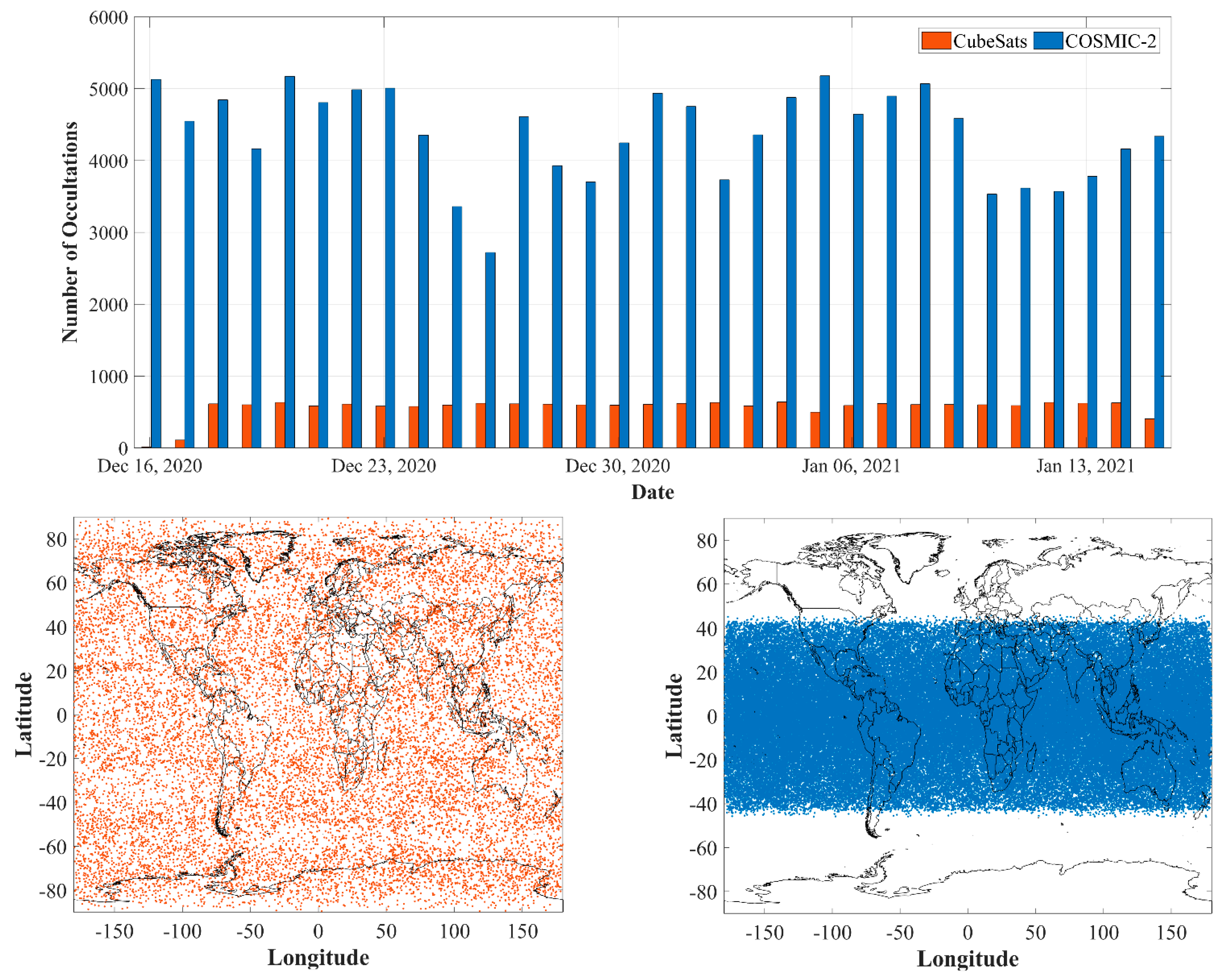
The RO atmospheric temperature profiles from the COSMIC-2 constellation and the data from the radiosonde observations, provided by the National Centers for Environmental Information (NCEI) through the Integrated Global Radiosonde Archive [68], are used to evaluate the CubeSats RO profiles derived from the SD excess phase in Equation (7). Available occultations from COSMIC-2 satellites and these 17 CubeSats over the testing period (16 Dec 2020 to 15 Jan 2021) are plotted in Figure 12 (top). Note that the number of occultations for the CubeSats is related to only 17 tested CubeSats and not all 145 CubeSats flying in the Spire Global constellation. Despite the Spire occultations being available for all ranges of latitudes (even from the only 17 tested CubeSats in Figure 12 (bottom left)), the COSMIC-2 does not provide the RO products for the high latitude and the polar regions (Figure 12 (bottom right)). This is mainly due to the type of the orbits and their inclinations as provided in Table 7. The second launch of the COSMIC-2 constellation with six satellites (COSMIC-2B) in higher inclined orbits (72°) was supposed to fill this gap; however, it was cancelled due to financial problems in building and launching these large LEO satellites [21]. This confirms the benefits of the affordable CubeSats compared with the expensive larger LEO satellites.

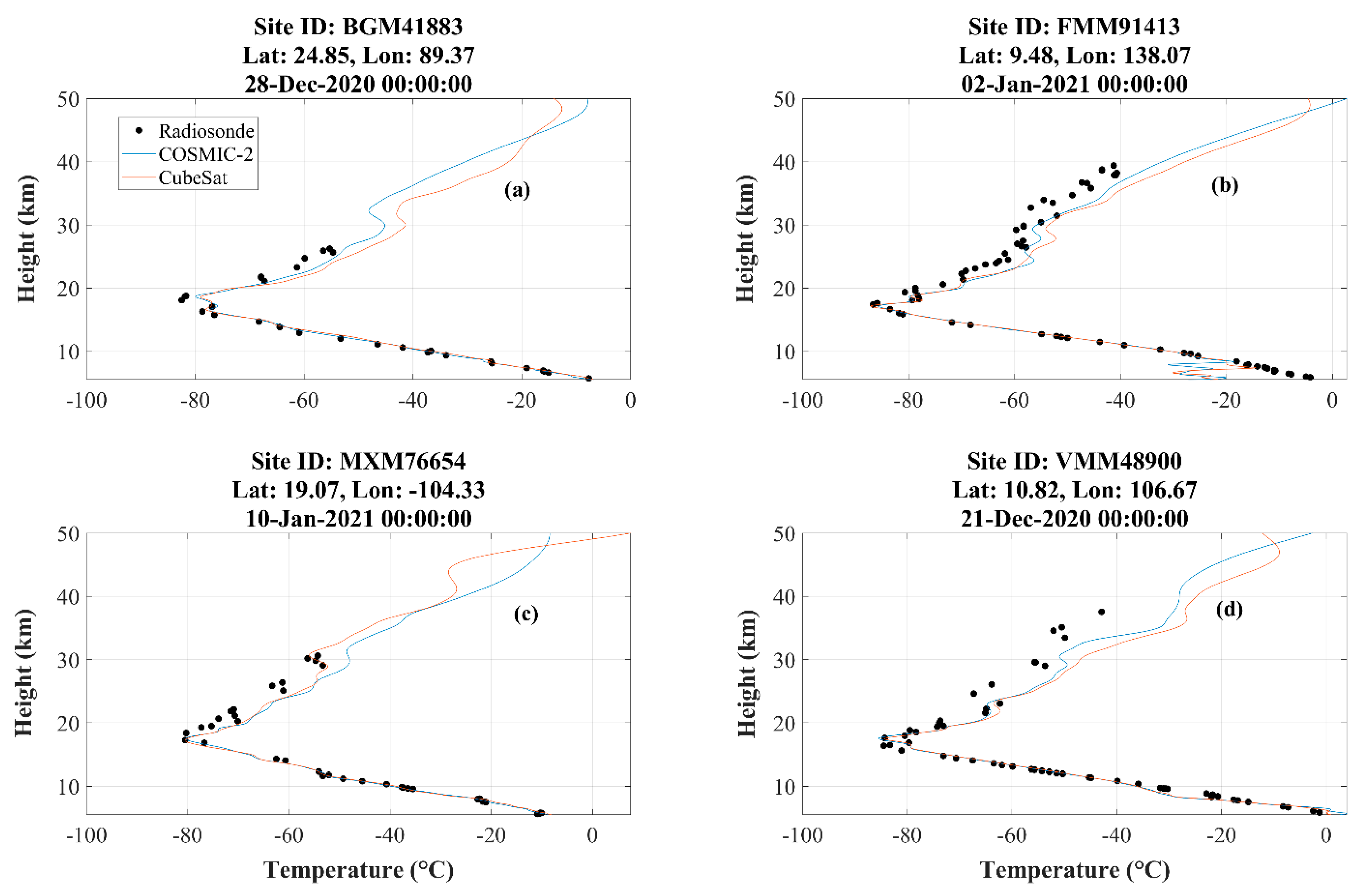
The radiosonde observations of four stations on four different dates are used to compare the temperature profiles. These radiosonde stations are located at Bogra in Bangladesh (BGM41883), Yap in the Caroline Islands (FMM91413), Manzanillo in Mexico (MXM76654), and Tan Son Hoa in Vietnam (VMM48900). Figure 13 compares the temperature profiles of CubeSats, COSMIC-2, and nearby radiosonde observations. Both CubeSats and COSMIC-2 profiles agree with the radiosonde observations to better than 1 °C for the vertical heights less than 20 km.

Table 8. Mean and standard deviation (STD) of the differences between the CubeSats and COSMIC-2 temperature values and the radiosonde observations for different heights.

Height (km)	CubeSats		COSMIC-2
	Mean (°C)	STD (°C)	Mean (°C)	STD (°C)
5–10	3.59	7.86	4.67	7.73
10–20	1.49	2.12	1.19	2.10
20–30	5.25	2.5	4.62	2.62
30–40	9.4	6.01	7.23	4.77

provides the mean and the standard deviation values for these agreements for different altitudes. The temperature values from both constellations are close to each other for the heights below 30 km, with the best temperature agreement observed around the UTLS (tropopause) region between 10 and 20 km, i.e., 1.49 and 1.19 °C for CubeSats and COSMIC-2, respectively. The differences for the heights above 30 km are large.

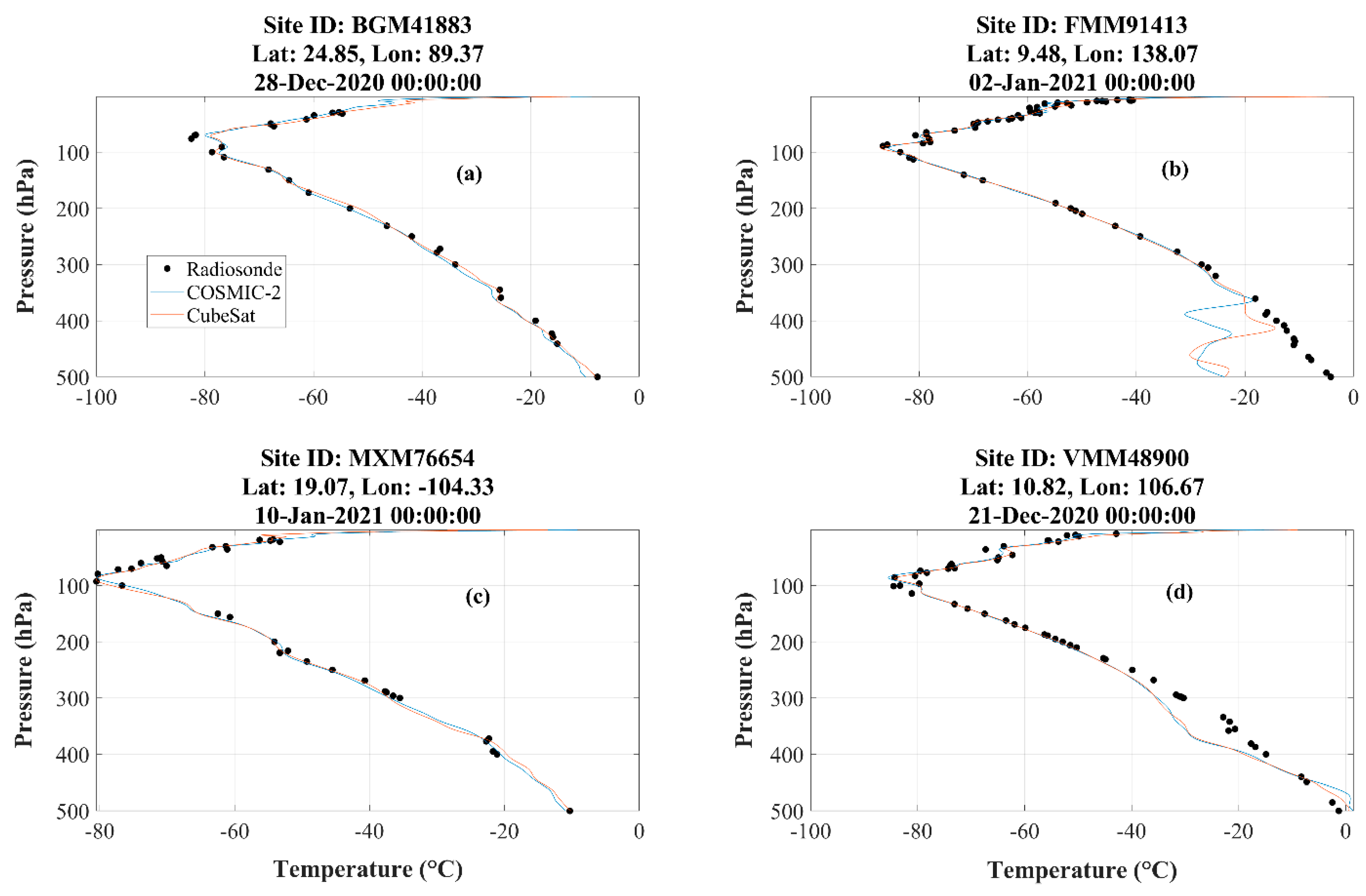
Additional evaluation of CubeSats’ derived GNSS-RO is obtained by plotting temperature versus pressure in Figure 14, which further shows the agreement between the CubeSats and the COSMIC-2 products compared to radiosonde observations. The agreements between the temperature values for pressures less than 300 hPa for CubeSats, COSMIC-2, and the radiosonde observations are obvious even with the visual inspection. However,

Table 9. Mean and standard deviation (STD) of the differences between CubeSats and COSMIC-2 temperature values and the radiosonde observations for different pressures levels.

Pressure (hPa)	CubeSats		COSMIC-2
	Mean (°C)	STD (°C)	Mean (°C)	STD (°C)
<100	0.12	2.77	0.68	2.81
100–300	0.54	1.69	0.63	1.61
300>	21.23	20.59	20.68	18.67

provides the means and standard deviations of this agreement. The perfect agreement of less than 0.1°C for the pressures less than 100 hPa is observed in the CubeSat data, which is even better than 0.68 °C for COSMIC-2. The large biases in the station FFM (Figure 14b) for the pressures higher than 300 hPa cause the large values of mean and the standard deviation of the temperature for that pressure range.

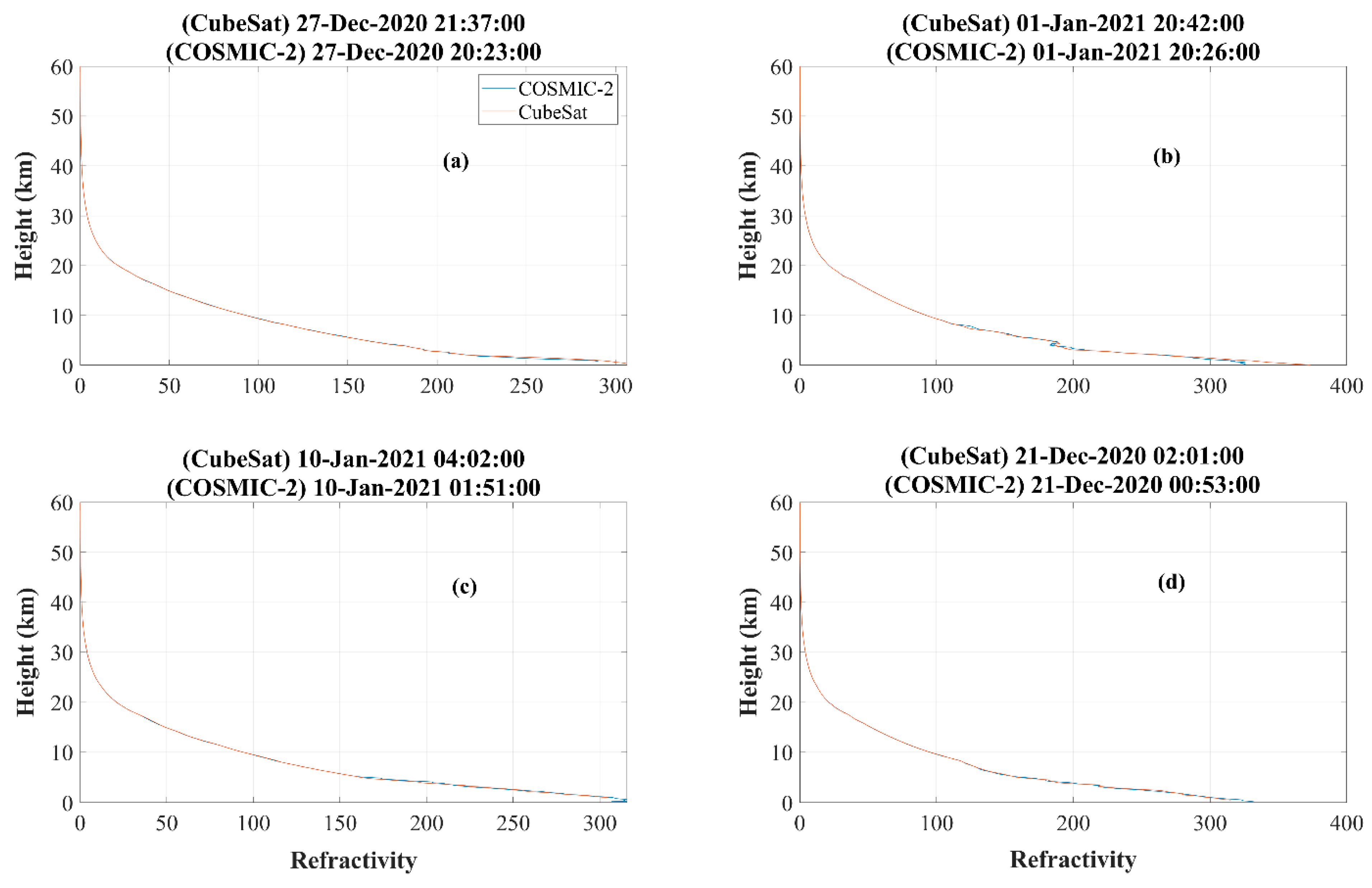
The refractivity comparisons between the CubeSats and the COSMIC-2 profiles for four random dates, i.e., 21 and 27 of December 2020 and 1 and 10 January 2021, are plotted in Figure 15. The RMS value for the differences between the refractivity from CubeSats and COSMIC-2 for the heights more than 10 km is 0.11, indicating an agreement between the two profiles. This value reaches 4.7 for heights lower than 10 km.

Finally, the Kling-Gupta Efficiency metric (KGE, Equation (9)) that combines the correlation ($C$), bias ($\beta$), and the variability ($\gamma$) is used to provide an overall performance of CubeSats and COSMIC-2 products against in situ radiosondes [69]:

$$KGE=1-\sqrt{{\left(C-1\right)}^2+{\left(\beta -1\right)}^2+{\left(\gamma -1\right)}^2}$$

(9)

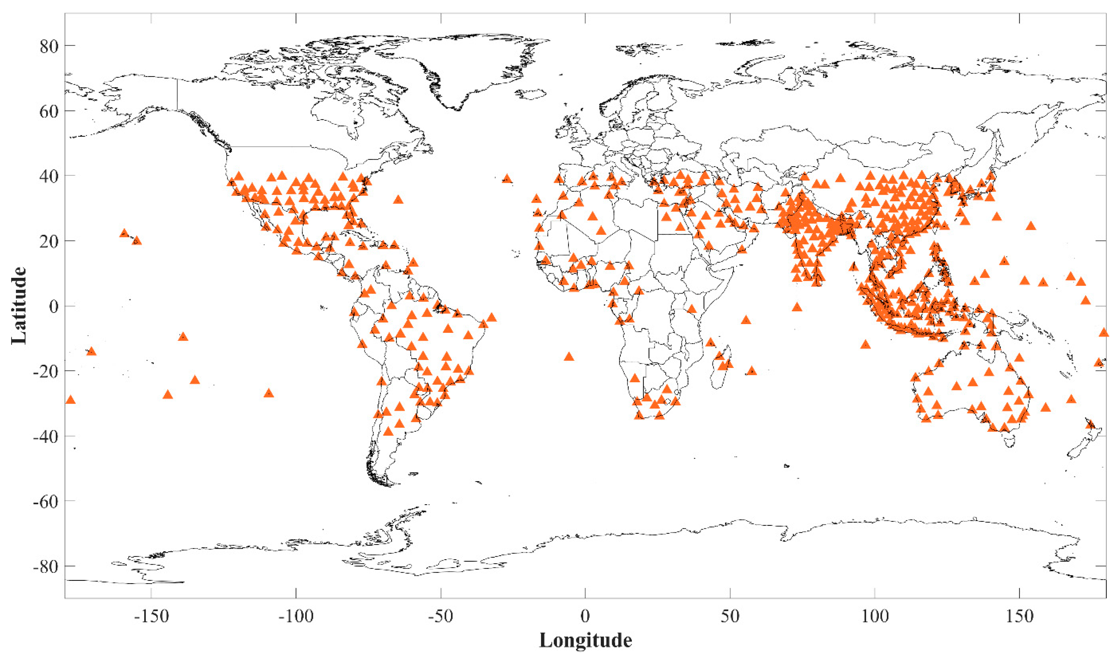
where $\beta =\frac{\mu }{{\mu }_0}$ is the ratio of the estimated and the observed mean, and $\gamma =\frac{\sigma /\mu }{{\sigma }_0/{\mu }_0}$ is the ratio of the estimated and observed variations derived from the means and the standard deviations. The radiosonde observations from 562 globally distributed stations shown in Figure 16 are used to compute the KGE values. To estimate the correlation, the observations from 50 stations co-located with the CubeSats and COSMIC-2 profiles are selected. Each pair of linear correlation is calculated between CubeSats, COSMIC-2, and radiosonde observations, and the mean of the correlation coefficient is used in Equation (9). The estimated KGE values for the CubeSats and the COSMIC-2 profiles against radiosonde observations are given in

Table 10. KGE values for the CubeSats and COSMIC-2 profiles against the radiosonde observations.

Profile	CubeSats	COSMIC-2
Height–Temperature	0.862	0.884
Pressure–Temperature	0.697	0.782

, where the values closer to 1 represent better agreement with the radiosonde observations. From the results in Table 10, it can be seen that CubeSats have close KGE values to COSMIC-2, thus indicating a good agreement of both products.

4. Summary and Conclusions

The stabilities of the CubeSats’ clocks that are estimated in the RD-POD procedure are important for high-rate applications such as GNSS-RO. These stabilities are affected by the following factors:

-

The ratio of the outliers in the observations derived from pre-processing steps;

-

The number of stochastic accelerations that are estimated in the POD procedure;

-

The CubeSats’ hardware biases due to, e.g., the thermal variations in space;

-

The nominal PCV values derived from ground calibration methods that do not consider the inflight situation;

-

The higher order of geopotential forces and their effects on relativity;

-

The quality of the frequency oscillator;

-

The float ambiguities and their impacts on the estimated clocks.

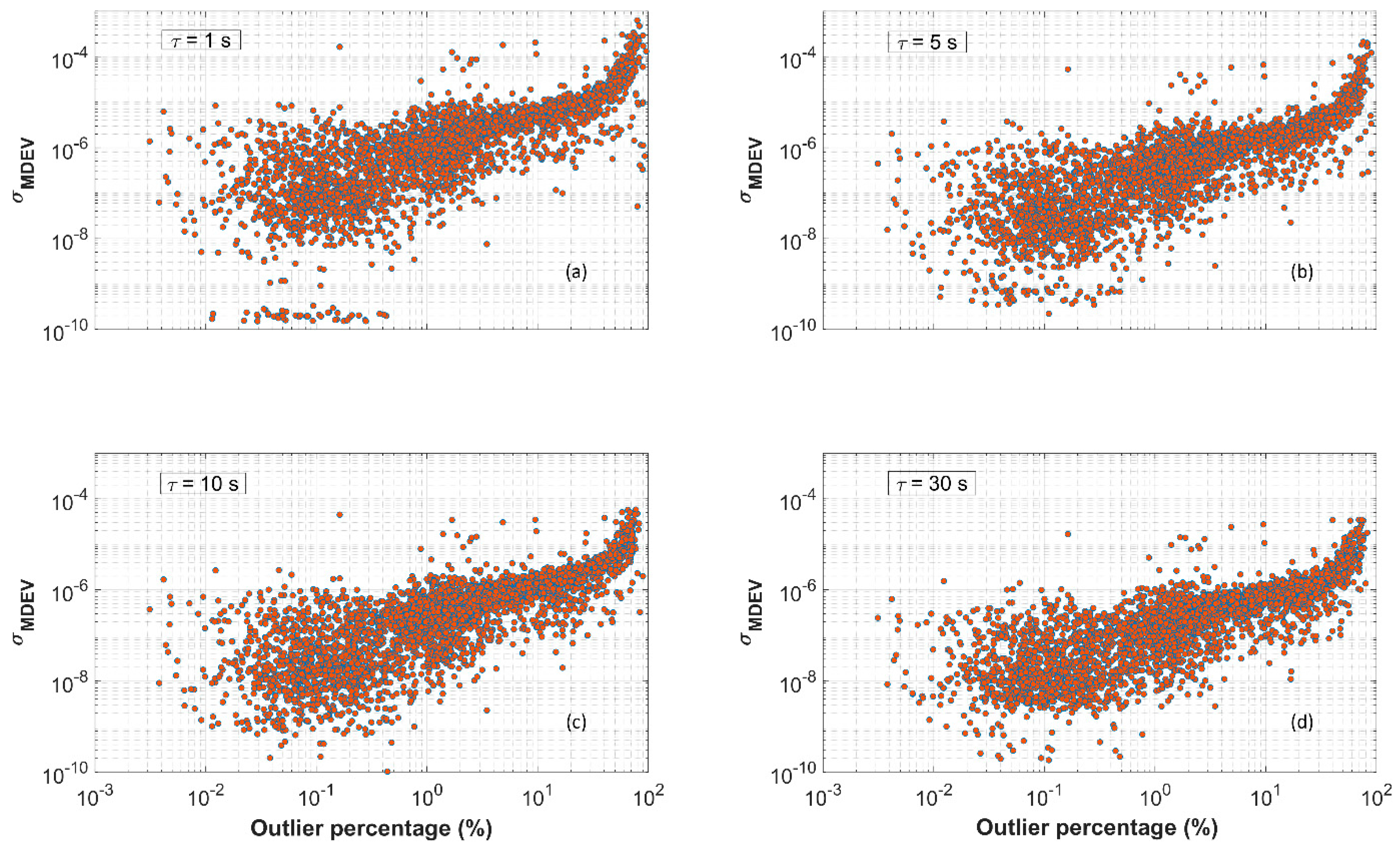
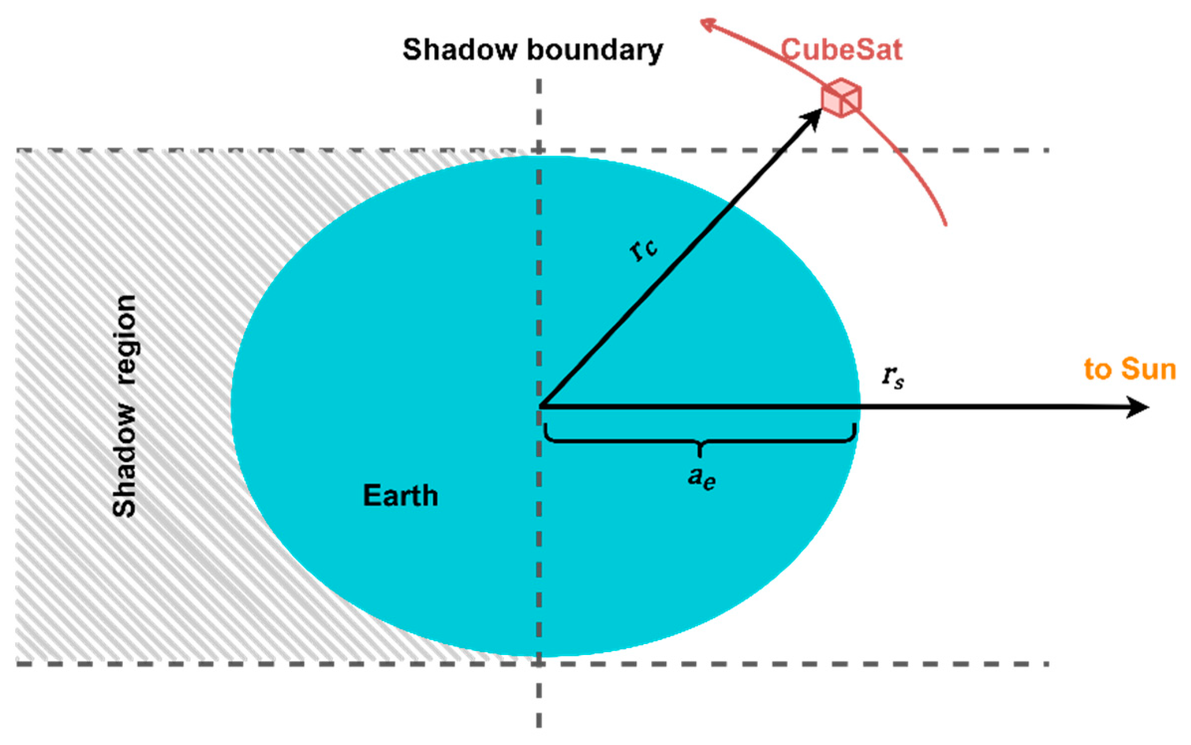
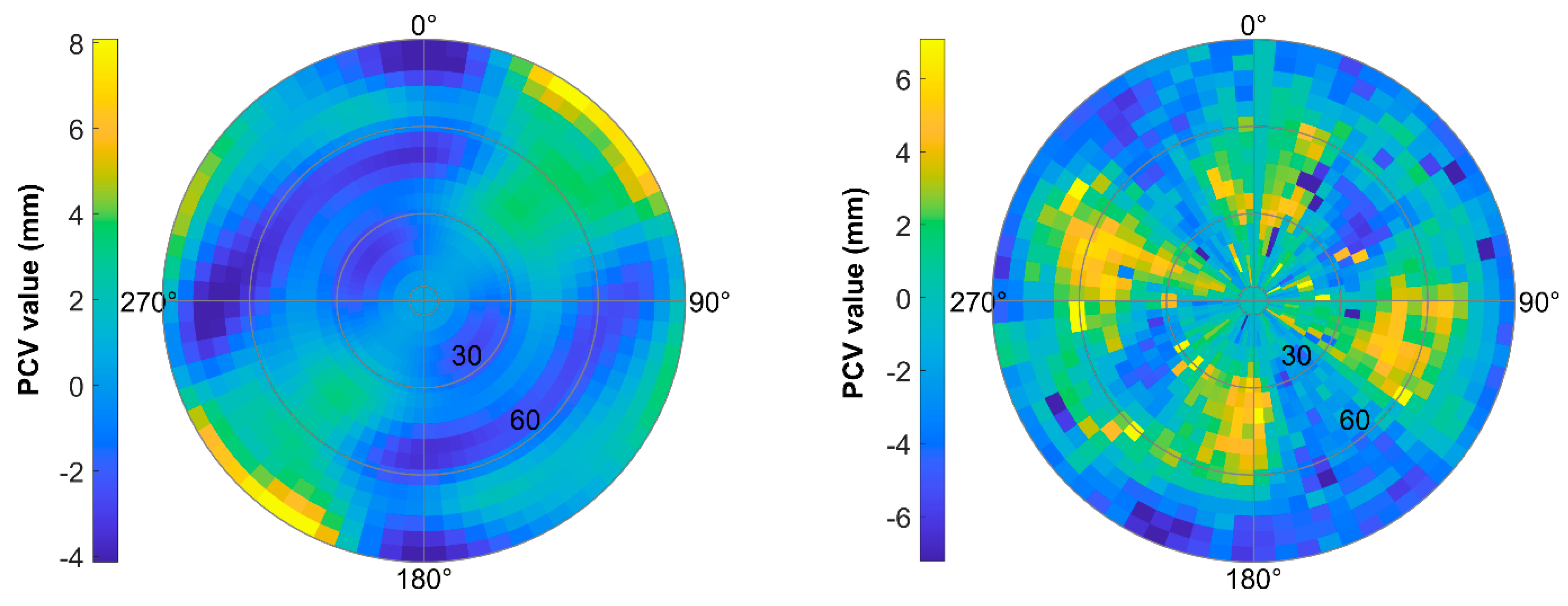
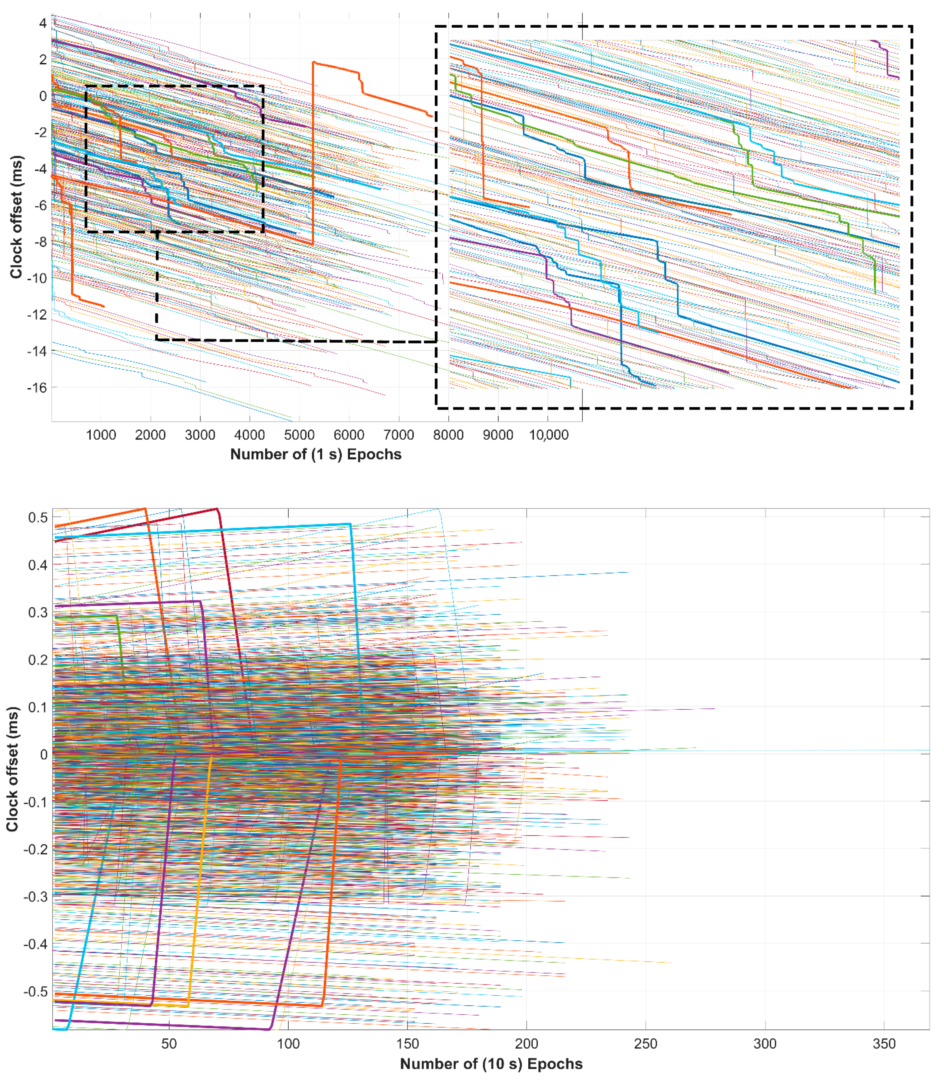
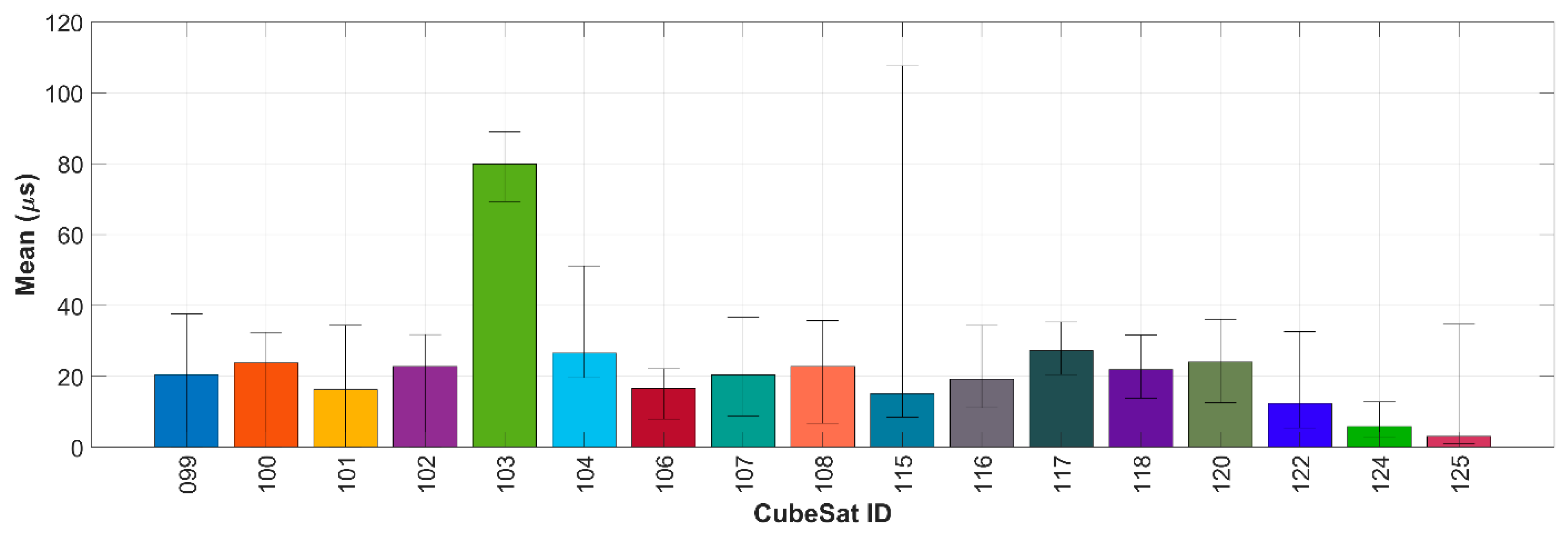
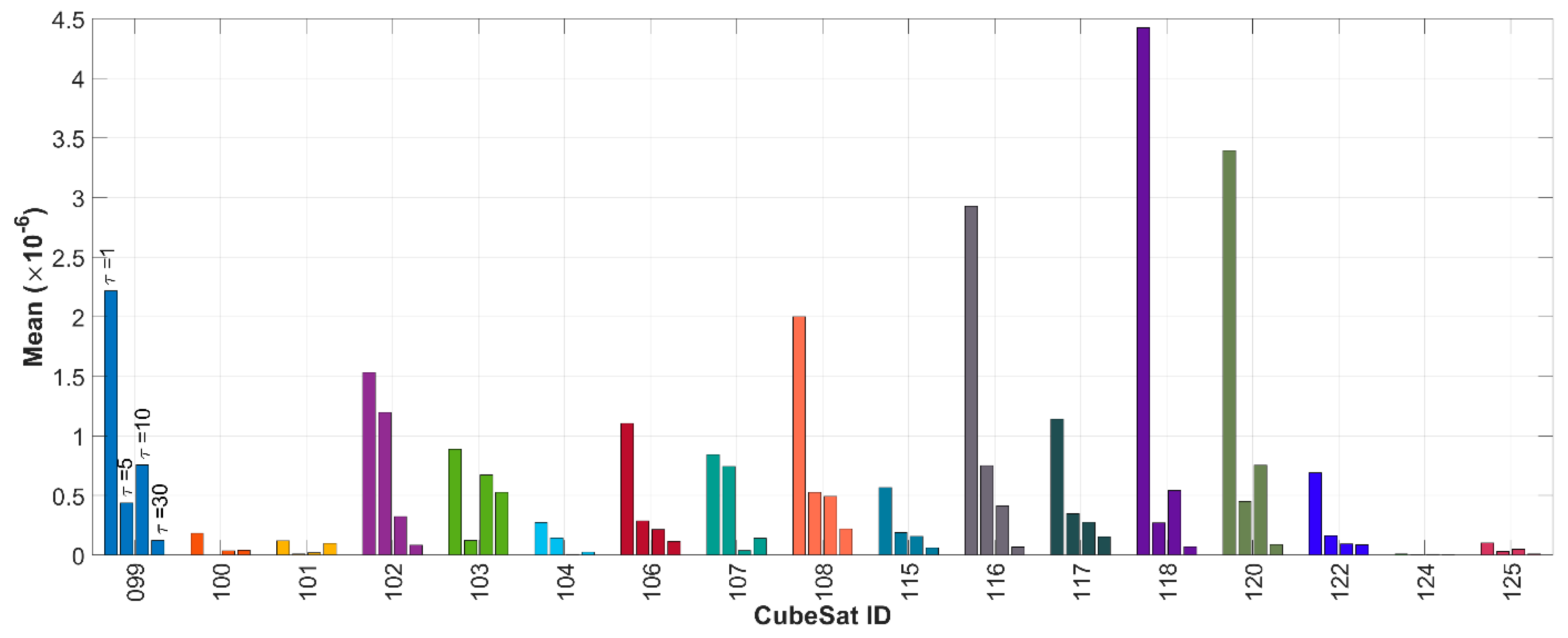
The impacts of these clock instability triggers were assessed for a set of CubeSats that have been launched for GNSS-RO. The stabilities of the CubeSats’ clocks are worse than ${10}^{-5}$ when the ratio of observation outliers is higher than 50%. This value can even drop to the ${10}^{-3}$ level for the high percentage of outliers (>90%). By increasing the number of stochastic accelerations including the estimation of velocity pulses at every 7.5 min and using constant accelerations for 3 min intervals, the short-term stabilities have been refined to the ${10}^{-8}$ to ${10}^{-6}$ level. To represent the impact of clock hardware biases due to thermal variations on the clock stabilities, a cylindrical shadow model was used to detect the CubeSat’s positions in the shadow of the earth, where the temperature drops and the direct sunlight as the dominant heat source is absent. The comparison of the estimated clocks for these regions with the clocks from the orbit in the sunlight revealed the impact of thermal variations on clock stabilities. Better thermal control systems may be required to handle the internal heat transfer between the COTS components of the CubeSats as well as the external heat sources. The new phase center variation (PCV) patterns are derived from the mean values of the observation residuals for different elevation and azimuth angles. Despite the nominal PCV values that are computed from ground calibrations, this pattern represents the actual multipath effect due to the CubeSat’s structure. The short-term stability improvements of the clocks after using this pattern varies from ${10}^{-11}$ to ${10}^{-9}$ for different CubeSats. Applying the J2 correction due to the earth’s oblateness in addition to the signal delays resulting from the central gravity and the clock deviations because of the relativity effect improves the CubeSat’s clock stability at the ${10}^{-11}$ to ${10}^{-8}$ level. In the analysis of the CubeSats’ clocks, several-millisecond-long jumps were observed, which seems to be due to the quality of the frequency oscillator. Such large jumps are not available for COSMIC-2 satellites that are equipped with ultra-stable oscillators. To show the impacts of all the aforementioned instability triggers, a final RD-POD round for all CubeSats is performed by applying all possible corrections together in the POD procedure. The results show improvements of several microseconds in the estimated clocks compared to the uncorrected clock estimations, thus confirming the improvement in the short-term stabilities after applying the proposed corrections. However, comparing with the COSMIC-2 clocks reveals the dominant role of the quality of the oscillators in the CubeSats’ clock instabilities. To deal with this limitation for the GNSS-RO application and derive the excess phase observations, single difference combinations between the reference GNSS satellite and the occulted one are formed. The integer ambiguity resolution in the POD procedure is among future studies and its impacts on the short-term stabilities are not investigated in this study. However, it is expected to be substantially less than the impact of the quality of the frequency oscillator.

The evaluations of the profiles derived from the CubeSats’ excess phase observations are in great agreement with those of the COSMIC-2 constellation, as well as the in situ radiosonde observations that provided an external validation source. The temperature profiles largely agree with those of COSMIC-2 at the UTLS (tropopause) region between 10 and 20 km, i.e., a mean of 1.49 ± 2.12 °C (CubeSats) and 1.19 ± 2.10 °C (COSMIC-2). The CubeSats (0.12 ± 2.77 °C) surprisingly outperformed the COSMIC-2 satellites (0.68 ± 2.81 °C) in the temperature-pressure profiles for the pressures less than 100 hPa. The refractivity comparisons between CubeSats and COSMIC-2 satellites show great agreements for heights more than 10 km. The KGE metrics for both CubeSats and COSMIC-2 in comparison with radiosonde observations are very close to each other, indicating CubeSats’ capability for atmospheric sounding. This level of quality and the fact that CubeSat constellations can cover the whole earth, including the high-altitude and polar regions, in contrast to COSMIC-2, show their importance in the future of GNSS-RO, which would be significant to numerical weather prediction models for global weather forecasting.

Although short-term stability and accuracy at the nanosecond level (or even better) can be derived by the availability of the chip-scale and miniature atomic clocks for the CubeSats, there are still some limitations that need more advancements in technology, such as increasing the processing power, as well as, in theory, providing more efficient algorithms for the onboard POD. This will be subject to future studies.

References

1. Feng, S.; Fu, Y.; Xiao, Q. Trends in the global tropopause thickness revealed by radiosondes. Geophys. Res. Lett. 2012, 39. [Google Scholar] [CrossRef]
2. Shangguan, M.; Wang, W.; Jin, S. Variability of temperature and ozone in the upper troposphere and lower stratosphere from multi-satellite observations and reanalysis data. Atmos. Chem. Phys. 2019, 19, 6659–6679. [Google Scholar] [CrossRef] [Green Version]
3. Xian, T.; Homeyer, C.R. Global tropopause altitudes in radiosondes and reanalyses. Atmos. Chem. Phys. 2019, 19, 5661–5678. [Google Scholar] [CrossRef] [Green Version]
4. Ruston, B.; Healy, S. Forecast Impact of FORMOSAT-7/COSMIC-2 GNSS Radio Occultation Measurements. Atmos. Sci. Lett. 2021, 22, e1019. [Google Scholar] [CrossRef]
5. Santer, B.D.; Wehner, M.F.; Wigley, T.M.L.; Sausen, R.; Meehl, G.A.; Taylor, K.E.; Ammann, C.; Arblaster, J.; Washington, W.M.; Boyle, J.S.; et al. Contributions of Anthropogenic and Natural Forcing to Recent Tropopause Height Changes. Science 2003, 301, 479–483. [Google Scholar] [CrossRef] [PubMed] [Green Version]
6. Santer, B.D.; Sausen, R.; Wigley, T.M.L.; Boyle, J.S.; AchutaRao, K.; Doutriaux, C.; Hansen, J.E.; Meehl, G.A.; Roeckner, E.; Ruedy, R.; et al. Behavior of tropopause height and atmospheric temperature in models, reanalyses, and observations: Decadal changes. J. Geophys. Res. Atmos. 2003, 108, ACL 1-1–ACL 1-22. [Google Scholar] [CrossRef] [Green Version]
7. Awange, J.L. Environmental Monitoring Using GNSS: Global Navigation Satellite Systems; Springer Science & Business Media: Amsterdam, The Netherlands, 2012. [Google Scholar] [CrossRef]
8. Awange, J. GNSS Environmental Sensing; Springer International Publishers: Amsterdam, The Netherlands, 2018; Volume 10, pp. 973–978. [Google Scholar] [CrossRef]
9. Awange, J.L.; Grafarend, E.W. GPS meteorology in environmental monitoring. In Solving Algebraic Computational Problems in Geodesy and Geoinformatics: The Answer to Modern Challenges; Awange, J.L., Grafarend, E.W., Eds.; Springer: Berlin/Heidelberg, Germany, 2005; pp. 217–244. [Google Scholar]
10. Elgered, G.; Wickert, J. Monitoring of the neutral atmosphere. In Springer Handbook of Global Navigation Satellite Systems; Teunissen, P.J.G., Montenbruck, O., Eds.; Springer International Publishing: Cham, Switzerland, 2017; pp. 1109–1138. [Google Scholar] [CrossRef]
11. Awange, J.; Kiema, J. Environmental Geoinformatics, Extreme Hydro-Climatic and Food Security Challenges: Exploiting the Big Data, 2nd ed.; Springer: Cham, Switzerland, 2019. [Google Scholar] [CrossRef]
12. Awange, J.; Kiema, J. Environmental Geoinformatics; Springer: Berlin/Heidelberg, Germany, 2013; pp. 973–978. [Google Scholar] [CrossRef]
13. Nascimento, A.A.; Awange, J.L.; Gonçalves, R.M.; Khandu. South America’s tropopause variability in relation to global teleconnection (2001–2017): A GNSS-radio occultation assessment. J. Atmos. Sol. Terr. Phys. 2020, 209, 105379. [Google Scholar] [CrossRef]
14. Wickert, J.; Schmidt, T.; Michalak, G.; Heise, S.; Arras, C.; Beyerle, G.; Falck, C.; König, R.; Pingel, D.; Rothacher, M. GPS Radio Occultation with CHAMP, GRACE-A, SAC-C, TerraSAR-X, and FORMOSAT-3/COSMIC: Brief Review of Results from GFZ. In New Horizons in Occultation Research: Studies in Atmosphere and Climate; Steiner, A., Pirscher, B., Foelsche, U., Kirchengast, G., Eds.; Springer: Berlin/Heidelberg, Germany, 2009; pp. 3–15. [Google Scholar]
15. von Engeln, A.; Andres, Y.; Marquardt, C.; Sancho, F. GRAS radio occultation on-board of Metop. Adv. Space Res. 2011, 47, 336–347. [Google Scholar] [CrossRef]
16. Schreiner, W.S.; Weiss, J.P.; Anthes, R.A.; Braun, J.; Chu, V.; Fong, J.; Hunt, D.; Kuo, Y.H.; Meehan, T.; Serafino, W.; et al. COSMIC-2 Radio Occultation Constellation: First Results. Geophys. Res. Lett. 2020, 47, e2019GL086841. [Google Scholar] [CrossRef]
17. Khandu; Awange, J.L.; Wickert, J.; Schmidt, T.; Sharifi, M.A.; Heck, B.; Fleming, K. GNSS remote sensing of the Australian tropopause. Clim. Chang. 2011, 105, 597–618. [Google Scholar] [CrossRef]
18. Yen, N. Status and Aims of the FORMOSAT-7/COSMIC-2 Mission. 2014. Available online: https://www.ecmwf.int/node/13747 (accessed on 1 November 2021).
19. Sarda, K.; Grant, C.; Eagleson, S.; Kekez, D.D.; Shah, A.; Zee, R.E. Canadian Advanced Nanospace Experiment 2: On-Orbit Experiences with a Three-Kilogram Satellite. In Proceedings of the AIAA/USU Conference on Small Satellites, Logan, UT, USA, 9–11 September 2008; Available online: https://www.worldcat.org/title/big-business-small-satellites-22nd-annual-aiaausu-conference-on-small-satellites-conference-proceedings-and-presentations-august-11-to-14-2007-logan-utah-usa/oclc/425278726 (accessed on 20 November 2021).
20. eoPortal-a. ARMADILLO (Attitude Related Maneuvers and Debris Instrument in Low (L) Orbit). Available online: https://directory.eoportal.org/web/eoportal/satellite-missions/a/armadillo (accessed on 25 August 2021).
21. eoPortal-b. STP-2-FormoSat-7/COSMIC-2. Available online: https://directory.eoportal.org/web/eoportal/satellite-missions/content/-/article/formosat-7 (accessed on 25 August 2021).
22. Bowler, N.E. An assessment of GNSS radio occultation data produced by Spire. Q. J. R. Meteorol. Soc. 2020, 146, 3772–3788. [Google Scholar] [CrossRef]
23. Montenbruck, O. Space applications. In Handbook of Global Navigation Satellite Systems; Teunissen, P.J.G., Montenbruck, O., Eds.; Springer: Cham, Switzerland, 2017; pp. 933–964. [Google Scholar] [CrossRef]
24. Allahvirdi-Zadeh, A.; El-Mowafy, A. Precise Orbit Determination of CubeSats Using a Proposed Observations Weighting Model. In Proceedings of the Scientific Assembly of the International Association of Geodesy (IAG), China Surveying and Mapping Mansion, Beijing, China, 28 June 2021. [Google Scholar] [CrossRef]
25. Wang, K.; El-Mowafy, A. LEO satellite clock analysis and prediction for positioning applications. Geo. Spat. Inf. Sci. 2021; in press. [Google Scholar] [CrossRef]
26. Tseng, T.-P.; Zhang, K.; Hwang, C.; Hugentobler, U.; Wang, C.-S.; Choy, S.; Li, Y.-S. Assessing antenna field of view and receiver clocks of COSMIC and GRACE satellites: Lessons for COSMIC-2. GPS Solut. 2014, 18, 219–230. [Google Scholar] [CrossRef]
27. Weinbach, U.; Schön, S. Improved GPS receiver clock modeling for kinematic orbit determination of the GRACE satellites. In Proceedings of the 2012 European Frequency and Time Forum, Gothenburg, Sweden, 23–27 April 2012; pp. 157–160. [Google Scholar] [CrossRef]
28. Tseng, T.-P.; Shum, C.K.; Yang, T.-Y. Characterizing receiver clock behaviors onboard Low Earth Orbiters: A case study of GRACE satellites. Geod. Geodyn. 2019, 10, 276–281. [Google Scholar] [CrossRef]
29. Poghosyan, A.; Golkar, A. CubeSat evolution: Analyzing CubeSat capabilities for conducting science missions. Prog. Aerosp. Sci. 2017, 88, 59–83. [Google Scholar] [CrossRef]
30. Selva, D.; Krejci, D. A survey and assessment of the capabilities of Cubesats for Earth observation. Acta Astronaut. 2012, 74, 50–68. [Google Scholar] [CrossRef]
31. Warren, Z.; Huang, M.; Kettering, H.; Stapleton, A.; Camparo, J. A versatile testbed for CubeSat atomic clock development: EOM vs Laser Current Modulation. In Proceedings of the 49th Annual Precise Time and Time Interval Systems and Applications Meeting, Reston, VA, USA, 1–29 January 2018; pp. 100–106. [Google Scholar] [CrossRef]
32. Rybak, M.M.; Axelrad, P.; Seubert, J.; Ely, T. Estimation of Thermal and Stochastic Variations of Chip Scale Atomic Clocks for Navigation of a Lunar CubeSat. In Proceedings of the 51st Annual Precise Time and Time Interval Systems and Applications Meeting, San Diego, CA, USA, 21–24 January 2020; pp. 221–233. [Google Scholar] [CrossRef]
33. Hajj, G.A.; Kursinski, E.R.; Romans, L.J.; Bertiger, W.I.; Leroy, S.S. A technical description of atmospheric sounding by GPS occultation. J. Atmos. Sol. Terr. Phys. 2002, 64, 451–469. [Google Scholar] [CrossRef]
34. Allahvirdi-Zadeh, A.; Wang, K.; El-Mowafy, A. Precise Orbit Determination of LEO Satellites Based on Undifferenced GNSS Observations. J. Surv. Eng. 2022, 148, 03121001. [Google Scholar] [CrossRef]
35. Wang, K.; Allahvirdi-Zadeh, A.; El-Mowafy, A.; Gross, J.N. A Sensitivity Study of POD Using Dual-Frequency GPS for CubeSats Data Limitation and Resources. Remote. Sens. 2020, 12, 2107. [Google Scholar] [CrossRef]
36. Montenbruck, O.; Gill, E. Satellite Orbits: Models, Methods and Applications; Springer: Berlin/Heidelberg, Germany, 2000. [Google Scholar] [CrossRef]
37. Dach, R.; Lutz, S.; Walser, P.; Fridez, P. Bernese GNSS Software, version 5.2; Bern Open Publishing: Bern, Switzerland, 2015. [Google Scholar]
38. Pavlis, N.; Kenyon, S.; Factor, J.; Holmes, S. Earth gravitational model 2008. In SEG Technical Program Expanded Abstracts 2008; SEG Technical Program Expanded Abstracts; Society of Exploration Geophysicists: Tulsa, OK, USA, 2008; pp. 761–763. [Google Scholar] [CrossRef]
39. Lyard, F.; Lefevre, F.; Letellier, T.; Francis, O. Modelling the global ocean tides: Modern insights from FES2004. Ocean Dynam. 2006, 56, 394–415. [Google Scholar] [CrossRef]
40. Petit, G.; Luzum, B. IERS Conventions. 2010. Available online: https://www.iers.org/IERS/EN/Publications/TechnicalNotes/tn36.html (accessed on 1 November 2021).
41. Standish, E. JPL Planetary and Lunar Ephemerides, DE405/LE405, JPL IOM 312. F-98_048 1998. Available online: https://ipnpr.jpl.nasa.gov/progress_report/42-196/196C.pdf (accessed on 1 November 2021).
42. Allahverdi-Zadeh, A.; Asgari, J.; Amiri-Simkooei, A.R. Investigation of GPS draconitic year effect on GPS time series of eliminated eclipsing GPS satellite data. J. Geod. Sci. 2016, 6, 93–102. [Google Scholar] [CrossRef]
43. Rothacher, M.; Schmid, R. ANTEX: The Antenna Exchange Format Version 1.4. Format Specification; IGS Central Bureau: Pasadena, CA, USA, 2010. [Google Scholar]
44. Bock, H.; Dach, R.; Jäggi, A.; Beutler, G. High-rate GPS clock corrections from CODE: Support of 1 Hz applications. J. Geod. 2009, 83, 1083. [Google Scholar] [CrossRef] [Green Version]
45. Weiss, J.P.; Steigenberger, P.; Springer, T. Orbit and clock product generation. In Springer Handbook of Global Navigation Satellite Systems; Teunissen, P.J.G., Montenbruck, O., Eds.; Springer International Publishing: Cham, Switzerland, 2017; pp. 983–1010. [Google Scholar] [CrossRef]
46. Allahvirdi-Zadeh, A.; Wang, K.; El-Mowafy, A. POD of small LEO satellites based on precise real-time MADOCA and SBAS-aided PPP corrections. GPS Solut. 2021, 25, 31. [Google Scholar] [CrossRef]
47. Griggs, E.; Kursinski, E.R.; Akos, D. Short-term GNSS satellite clock stability. Radio Sci. 2015, 50, 813–826. [Google Scholar] [CrossRef]
48. Tseng, T.-P.; Chen, S.-Y.; Chen, K.-L.; Huang, C.-Y.; Yeh, W.-H. Determination of near real-time GNSS satellite clocks for the FORMOSAT-7/COSMIC-2 satellite mission. GPS Solut. 2018, 22, 47. [Google Scholar] [CrossRef]
49. Riley, W.J. Handbook of Frequency Stability Analysis; US Department of Commerce, National Institute of Standards and Technology. 2008. Available online: https://safe.nrao.edu/wiki/pub/Main/ToddHunter/nist1065.pdf (accessed on 1 November 2021).
50. Kroes, R. Precise Relative Positioning of Formation Flying Spacecraft Using GPS. Optima Grafische Communicatie, PO Box 84115, 3009 BC Rotterdam, The Netherlands. 2006. Available online: https://www.ncgeo.nl/downloads/61Kroes.pdf (accessed on 1 November 2021).
51. Wang, L.; Chen, R.; Li, D.; Zhang, G.; Shen, X.; Yu, B.; Wu, C.; Xie, S.; Zhang, P.; Li, M. Initial assessment of the LEO based navigation signal augmentation system from Luojia-1A satellite. Sensors 2018, 18, 3919. [Google Scholar] [CrossRef] [Green Version]
52. Gilmore, D.G.; Donabedian, M. Spacecraft Thermal Control Handbook: Cryogenics; AIAA: Reston, VA, USA, 2002; Volume 2. [Google Scholar]
53. Boushon, K.E. Thermal Analysis and Control of Small Satellites in Low Earth Orbit. M.S.A.E.; Missouri University of Science and Technology: Ann Arbor, MI, USA, 2018. [Google Scholar]
54. Hauschild, A.; Montenbruck, O. Real-time clock estimation for precise orbit determination of LEO-satellites. In Proceedings of the 21st International Technical Meeting of the Satellite Division of The Institute of Navigation (ION GNSS 2008), Savannah, GA, USA, 16–19 September 2008; pp. 581–589. [Google Scholar]
55. Pirazzi, G.; Mazzoni, A.; Biagi, L.; Crespi, M. Preliminary performance analysis with a GPS+ Galileo enabled chipset embedded in a smartphone. In Proceedings of the 30th International Technical Meeting of the Satellite Division of The Institute of Navigation (ION GNSS+ 2017), Portland, OR, USA, 25–29 September 2017; pp. 101–115. [Google Scholar] [CrossRef]
56. Svehla, D. Geometrical Theory of Satellite Orbits and Gravity Field; Springer: Berlin/Heidelberg, Germany, 2018. [Google Scholar] [CrossRef] [Green Version]
57. Jäggi, A.; Dach, R.; Montenbruck, O.; Hugentobler, U.; Bock, H.; Beutler, G. Phase center modeling for LEO GPS receiver antennas and its impact on precise orbit determination. J. Geod. 2009, 83, 1145. [Google Scholar] [CrossRef] [Green Version]
58. Allahvirdi-Zadeh, A. Phase centre variation of the GNSS antenna onboard the CubeSats and its impact on precise orbit determination. In Proceedings of the GSA Earth Sciences Student Symposium, Western Australia (GESSS-WA), Perth, Australia, 25 November 2021. [Google Scholar] [CrossRef]
59. Ashby, N. Relativity in the Global Positioning System. Living Rev. Relativ. 2003, 6, 1–42. [Google Scholar] [CrossRef] [PubMed] [Green Version]
60. Hauschild, A. Basic observation equations. In Springer Handbook of Global Navigation Satellite Systems; Teunissen, P.J.G., Montenbruck, O., Eds.; Springer International Publishing: Cham, Switzerland, 2017; pp. 561–582. [Google Scholar] [CrossRef]
61. UCAR. UCAR COSMIC Program, COSMIC-2 Data Products Near Real-Time Operational Datasets. UCAR/NCAR-COSMIC. 2019. Available online: https://www.cosmic.ucar.edu/what-we-do/cosmic-2/data/ (accessed on 28 October 2021).
62. Beyerle, G.; Schmidt, T.; Michalak, G.; Heise, S.; Wickert, J.; Reigber, C. GPS radio occultation with GRACE: Atmospheric profiling utilizing the zero difference technique. Geophys. Res. Lett. 2005, 32. [Google Scholar] [CrossRef] [Green Version]
63. Weiss, J.-P. FORMOSAT-7/COSMIC-2 Neutral Atmosphere Initial Operating Capability Data Release. 2020. Available online: https://data.cosmic.ucar.edu/gnss-ro/cosmic2/nrt/F7C2_NA_IOC_Data_Release_Memo.pdf. (accessed on 1 November 2021).
64. Weiss, J.-P.; Hunt, D.; Schreiner, W.; VanHove, T.; Arnold, D.; Jaeggi, A. COSMIC-2 Precise Orbit Determination Results. In Proceedings of the EGU General Assembly Conference Abstracts 2020, Online, 4–8 May 2020. [Google Scholar]
65. Li, Y.; Hwang, C.; Tseng, T.; Huang, C.; Bock, H. A Near-Real-Time Automatic Orbit Determination System for COSMIC and Its Follow-On Satellite Mission: Analysis of Orbit and Clock Errors on Radio Occultation. IEEE Trans. Geosci. Remote Sens. 2014, 52, 3192–3203. [Google Scholar] [CrossRef]
66. Xia, P.; Ye, S.; Jiang, K.; Chen, D. Estimation and evaluation of COSMIC radio occultation excess phase using undifferenced measurements. Atmos. Meas. Tech. 2017, 10, 1813–1821. [Google Scholar] [CrossRef] [Green Version]
67. Conklin, J.W.; Nydam, S.; Ritz, T.; Barnwell, N.; Serra, P.; Hanson, J.; Nguyen, A.N.; Priscal, C.; Stupl, J.; Jaroux, B. Preliminary results from the chomptt laser time-transfer mission. In Proceedings of the 3rd Annual AIAA/USU Conference on Small Satellites, Logan, UT, USA, 6 August 2019. [Google Scholar]
68. IGRA. Integrated Global Radiosonde Archive. 2021. Available online: https://www.ncei.noaa.gov/products/weather-balloon/integrated-global-radiosonde-archive (accessed on 1 November 2021).
69. Gupta, H.V.; Kling, H.; Yilmaz, K.K.; Martinez, G.F. Decomposition of the mean squared error and NSE performance criteria: Implications for improving hydrological modelling. J. Hydrol. 2009, 377, 80–91. [Google Scholar] [CrossRef] [Green Version]
Figure 1. Structure of the Spire 3U RO CubeSat (source: Spire Global, Inc.).
Remotesensing 14 00362 g001
Figure 2. MDEV of the estimated clocks of all 17 CubeSats from the RD-POD over the testing period (31 days: 16 December 2020–15 January 2021). Different colours are dedicated to the different observation segments.
Remotesensing 14 00362 g002
Figure 3. Flowchart indicating CubeSats’ clock instability assessment and the proposed remedies.
Remotesensing 14 00362 g003
Figure 4. MDEV of the 17 CubeSats’ clocks for short averaging times plotted against the percentage of the observations that are considered outliers in the pre-processing steps. In the subfigures, each dot represents the MDEV of one observation segment for one CubeSat over the testing period. The subfigures (ad) indicate averaging times 1, 5, 10, and 30 s, respectively.
Remotesensing 14 00362 g004
Figure 5. Cylindrical model for detecting CubeSats located in the shadow of the earth.
Remotesensing 14 00362 g005
Figure 6. PCV patterns with 5° resolution for the CubeSat antenna (Lemur 3.1.0) from the antenna calibration (left) and the inflight observations using the residual approach (right). The inner circles are marked with the elevation angles, and the azimuth values are tagged on the outer circle. The azimuth 0° coincides with the positive x-axis of the CubeSats’ body frame (approximately the positive velocity direction) in the zero-quaternion case.
Remotesensing 14 00362 g006
Figure 7. Estimated clock offsets from all observation segments of CubeSat 099 (top) and COSMIC-2A 1 (bottom) over the testing period. Several millisecond jumps are observed for CubeSat’s oscillator compared to the USO’s onboard COSMIC-2. Some of the clocks are plotted in bold for better visibility.
Remotesensing 14 00362 g007
Figure 8. Mean of the improvements in comparing the estimated CubeSats’ clocks before and after applying the proposed corrections in the RD-POD procedure. The lines inside each bar show the minimum and maximum RMS of the improvements over the testing period.
Remotesensing 14 00362 g008
Figure 9. Mean of the MDEV reductions in the short-term stabilities after applying the proposed corrections compared to the first estimation of clocks, i.e., before applying the proposed remedies. Each CubeSat has four bars related to short averaging times (1, 5, 10, and 30 s, respectively). They are tagged for CubeSat 099 as an example.
Remotesensing 14 00362 g009
Figure 10. MDEV of the estimated clocks of COSMIC-2 satellites. Different colours are dedicated to the different observation segments of each COSMIC-2 satellite. The duration of the observation segments is varied from 30 min to 2 h, generally around 1.5 h with a sample interval of 10 s.
Remotesensing 14 00362 g010
Figure 11. COSMIC-2 satellite structure (credit: Surrey Satellite Technology).
Remotesensing 14 00362 g011
Figure 12. Number of occultations for the COSMIC-2 constellation and 17 CubeSats (top), Geographical coverage of the 17 tested CubeSats (bottom left), and COSMIC-2 constellation (bottom right) over the testing period (16 December 2020–15 January 2021).
Remotesensing 14 00362 g012
Figure 13. Comparing the CubeSats and COSMIC-2 with radiosonde observations as a reference in terms of temperature and height. The profiles related to each site are provided in subfigures (ad).
Remotesensing 14 00362 g013
Figure 14. Comparing CubeSats and COSMIC-2 with the radiosonde observations as a reference in terms of the temperature and pressure. The profiles related to each site are provided in subfigures (ad).
Remotesensing 14 00362 g014
Figure 15. Comparing CubeSats and COSMIC-2 in terms of the refractivity and height. The profiles related to each date are provided in subfigures (ad).
Remotesensing 14 00362 g015
Figure 16. Locations of the radiosonde stations used for the validation using KGE metric.
Remotesensing 14 00362 g016