Article

Integrity Monitoring of PPP-RTK Positioning; Part II: LEO Augmentation

1
National Time Service Center, Chinese Academy of Sciences, Xi’an 710600, China
2
University of Chinese Academy of Sciences, Beijing 100049, China
3
School of Earth and Planetary Sciences, Curtin University, Perth, WA 6845, Australia
4
Beijing Future Navigation Technology Co., Ltd., Beijing 100094, China
*
Author to whom correspondence should be addressed.
Remote Sens. 2022, 14(7), 1599; https://doi.org/10.3390/rs14071599
Submission received: 3 February 2022 / Revised: 20 March 2022 / Accepted: 23 March 2022 / Published: 26 March 2022
(This article belongs to the Special Issue LEO-Augmented PNT Service)

Abstract

:
Low Earth orbit (LEO) satellites benefit future ground-based positioning with their high number, strong signal strength and high speed. The rapid geometry change with the LEO augmentation offers acceleration of the convergence of the precision point positioning (PPP) solution. This contribution discusses the influences of the LEO augmentation on the precise point positioning—real-time kinematic (PPP-RTK) positioning and its integrity monitoring. Using 1 Hz simulated data around Beijing for global positioning system (GPS)/Galileo/Beidou navigation satellite system (BDS)-3 and the tested LEO constellation with 150 satellites on L1/L5, it was found that the convergence of the formal horizontal precision can be significantly shortened in the ambiguity-float case, especially for the single-constellation scenarios with low precision of the interpolated ionospheric delays. The LEO augmentation also improves the efficiency of the user ambiguity resolution and the formal horizontal precision with the ambiguities fixed. Using the integrity monitoring (IM) procedure introduced in the first part of this series of papers, the ambiguity-float horizontal protection levels (HPLs) are sharply reduced in various tested scenarios, with an improvement of more than 60% from 5 to 30 min after the processing start. The ambiguity-fixed HPLs can generally be improved by 10% to 60% with the LEO augmentation, depending on the global navigation satellite system (GNSS) constellations used and the precision of the ionospheric interpolation.

Graphical Abstract

1. Introduction

Low Earth orbit (LEO) satellites have been frequently discussed for the positioning, navigation and timing (PNT) service in recent years. Compared with the medium Earth orbit (MEO) and geostationary (GEO) satellites of different global navigation satellite systems (GNSSs), LEO satellites exhibit their advantages in their large number, low altitude, fast speed and strong signal strength [1]. The increased number of satellites improves their geometry and the redundancy of observations, which benefits positioning and timing precision in general [2]. The low altitude and the corresponding high speed of LEO satellites enable a much faster geometry change and hereby significantly shorten the convergence time for precise point positioning (PPP) [3,4,5]. The fast speed of the LEO satellites, in addition, whitens the multipath effects that have been a bottleneck for GNSS positioning in complicated measurement environments [6]. Compared to the GNSS satellites, LEO satellites’ much stronger signal strength allows their signals to penetrate obstacles, which enlarges the limited satellite visibility in areas surrounded by high buildings, or even indoors [7]. Nevertheless, the LEO satellites also experience quick and short passes compared to the GNSS satellites [8], and suffer from lower elevation angles and smaller footprints [9].
The benefits of LEO augmentation have been frequently discussed to improve positioning performance. Its benefits in the integrity monitoring (IM) of the positional results, which finds more and more applications nowadays in the intelligent transport systems (ITSs), have been rarely discussed. In [10], LEO augmentation is shown to be able to improve the IM performance of the Beidou navigation satellite system (BDS). In [11], the IM of LEO precise orbit determination (POD) results were discussed. In this study, the focus is on the IM service for ground-based users, who will need the integration of LEO signals in their positioning activities in the near future.
Compared to the PPP method that has been a hot spot in many studies of the LEO-augmented PNT service, precise point positioning—real-time kinematic (PPP-RTK) positioning combines the advantage of the independency in the PPP and that of the integer ambiguity resolution (IAR) of the RTK [12,13]. It is thus considered as IAR-enabled PPP. In the first part of this series of papers [14], an IM procedure was proposed for GNSS-based PPP-RTK positioning. A pessimistic horizontal positional error bound, namely the horizontal protection level (HPL), was estimated under a given horizontal probability of misleading information, denoted as PMI H . The HPL was shown to be closely related to the ionosphere and multipath conditions. A low HPL tends to provide high IM availability, as the system becomes unavailable when HPL exceeds a pre-defined horizontal alert limit (HAL).
In this contribution, the influences of the LEO augmentation will be discussed based on the proposed IM procedure. Using the planned navigation-oriented LEO constellation of the CentiSpace in China [15], the changes brought by the LEO augmentation in the measurement geometry, the PPP-RTK positioning and the HPLs are discussed for both the ambiguity-fixed and -float cases. The analysis is performed when LEO satellites augment single-, dual- and triple-GNSS-constellations, i.e., the global positioning system (GPS), the Galileo and the BDS under the L1/L5 dual-frequency scenario. Different characteristics of LEO satellites are utilized to exhibit their influences on positioning and IM performances using the PPP-RTK method.
This paper starts with an introduction to the changes of the measurement geometry under the tested LEO augmentation. The processing strategy that was explained in the first part of this series of papers is shortly reviewed. Afterward, different issues for LEO-augmented PPP-RTK positioning are discussed in detail, with the focus put on the changes in the formal horizontal precision and the HPL. The conclusion is given at the end of the paper.

2. Measurement Geometry under LEO Augmentation

The GNSSs have experienced rapid development in the past decades. As of 1 February 2022, the GPS has 30 operational satellites, among which 16 are operational satellites transmitting signals on the L1 (1575.42 MHz), L2 (1227.6 MHz) and L5 (1176.45 MHz) for positioning and navigation purposes [16]. At the same time, the Galileo system of the European Union (EU) is also increasing its size and on its way to a full constellation, having 3 In-Orbit-Validation (IOV) satellites left operational in the system, and 19 Full Operational Capability (FOC) satellites usable by 1 February 2022. All the currently operational Galileo satellites are transmitting five-frequency signals on E1, E5a, E5, E5b and E6, which have overlapped frequencies on E1 and E5a with the GPS on L1 and L5. In 2020, the Chinese BDS completed its full constellation. Until 1 February 2022, it has 42 operational satellites, including 12 satellites of BDS-2 and the remaining 30 of BDS-3. In addition to 24 MEO satellites, different from the GPS and the Galileo, the BDS also has 8 Geostationary (GEO) satellites and 10 Inclined Geosynchronous orbit (IGSO) satellites. The BDS also occupies a relatively complicated frequency structure, having the BDS-2 satellites transmitting signals on B1I (1561.098 MHz), B2I (1207.14 MHz) and B3I (1268.52 MHz) and the BDS-3 satellites sending open signals in addition to B1I, B3I and also on B1C (1575.42 MHz), B2a (1176.45 MHz) and B2b (1207.14 MHz) [17]. The frequency structure of the three constellations is illustrated in Figure 1. It can be observed that the L1 of 1575.42 MHz and the L5 of 1176.45 MHz are the only two frequencies that are currently shared by all three systems.
For a dual-frequency user, Figure 1 also shows that the tracking combination of L1 and L5 would lead to a maximal number of usable satellites from these three systems, i.e., 68 in total. In addition to the satellite numbers, the signals on L5 were also shown to have smaller code noise [18] and to be more robust against interferences [19]. Due to all these advantages, these two frequencies are planned to be used for the US/EU dual-frequency multi-constellation (DFMC) positioning service in aviation, both for the case using the GNSS broadcast ephemeris with the advanced Receiver Autonomous Integrity Monitoring algorithm (ARAIM) [20,21], and the case using DFMC Satellite-Based Augmentation System (SBAS) corrections [22,23].

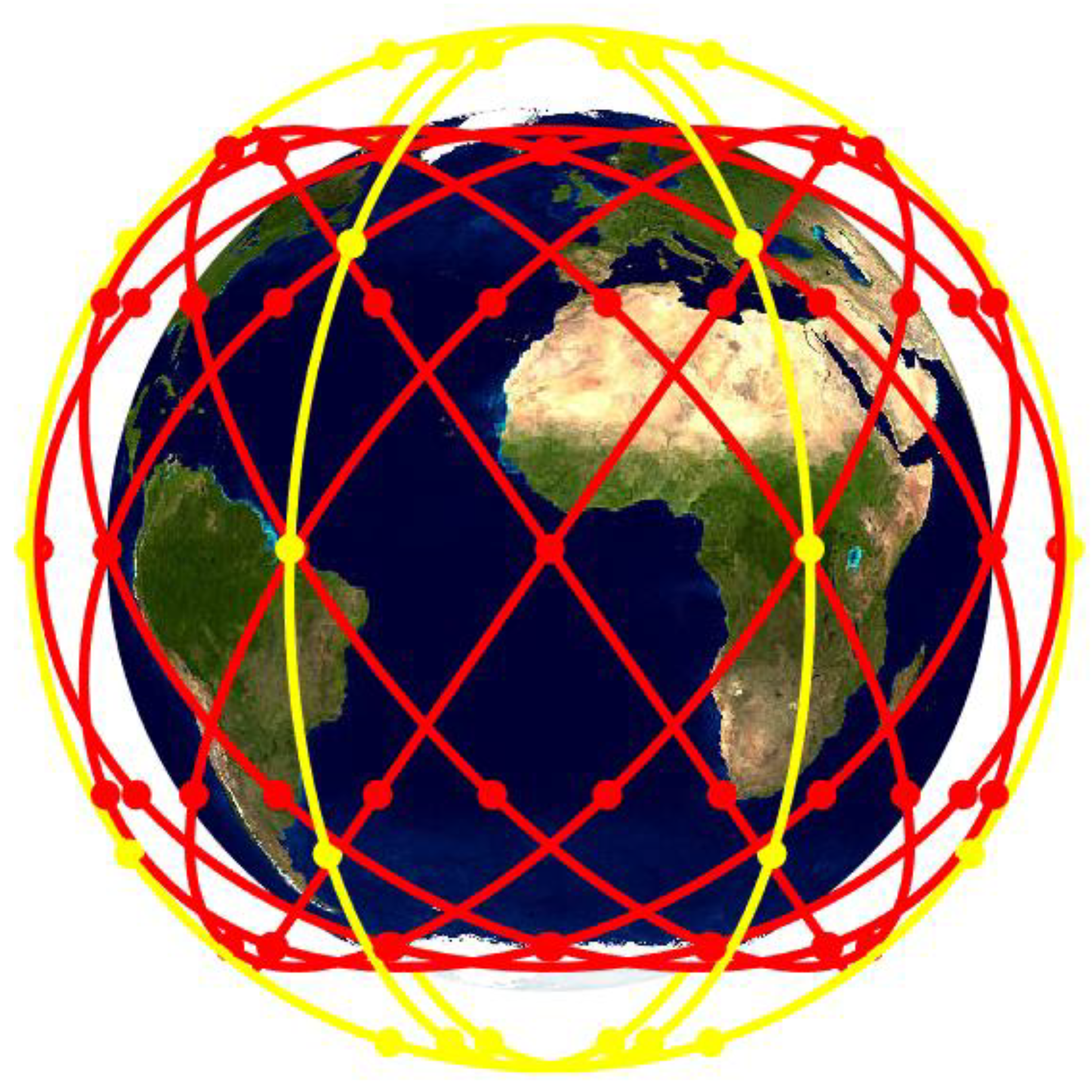
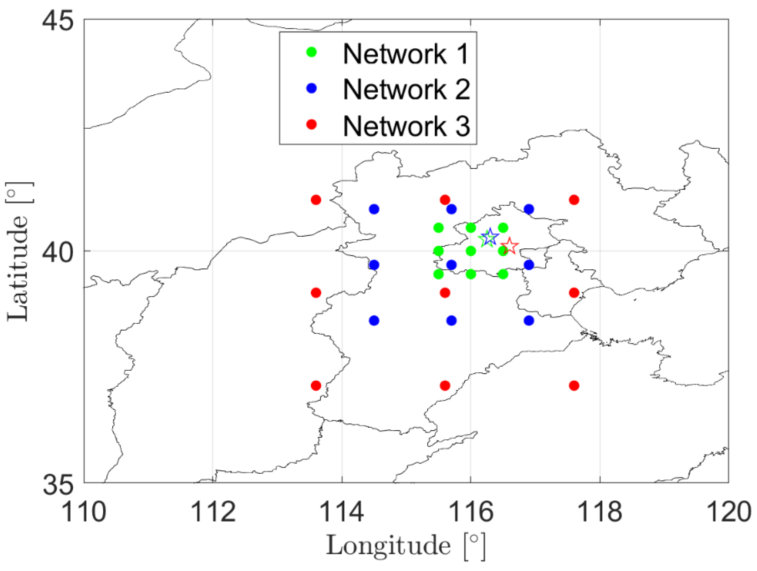
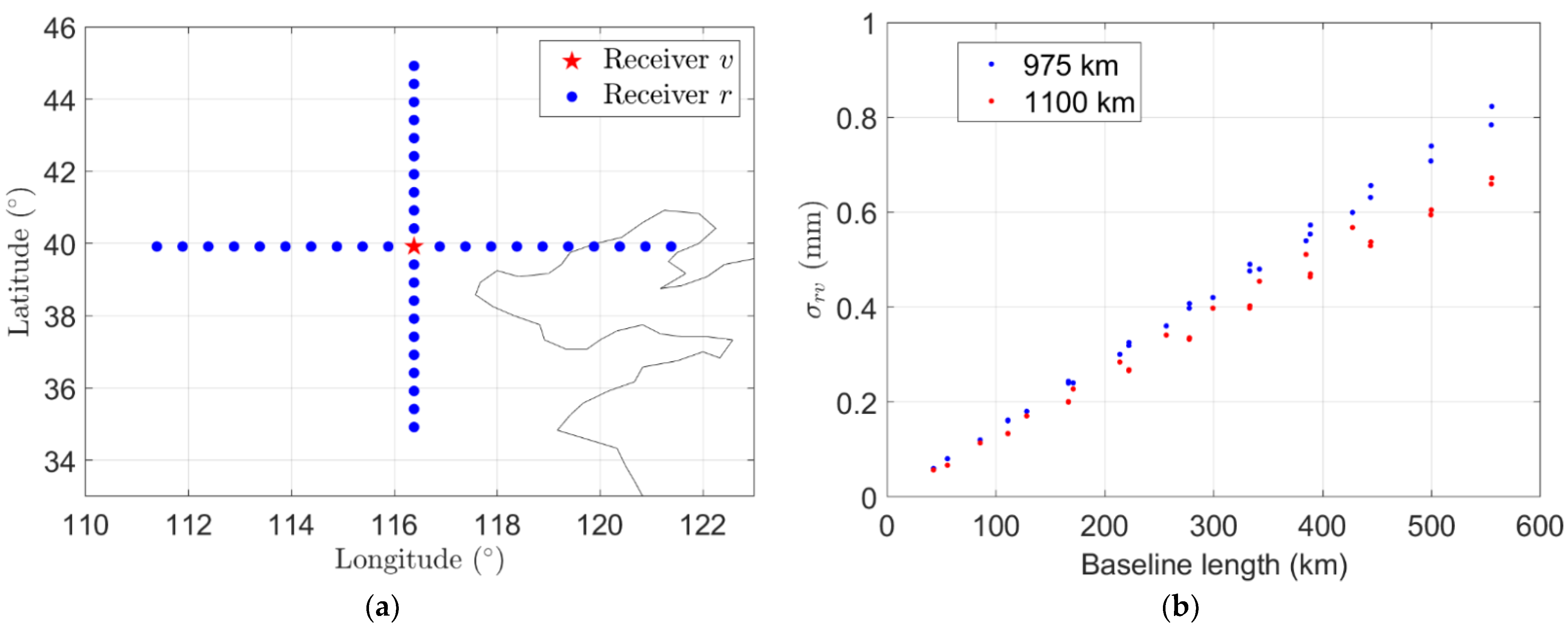
2.1. The LEO Configuration

Based on the various advantages provided by LEO satellites as mentioned in the introduction, some LEO satellite constellations have been designed for navigation purposes and considered as augmentation systems to GNSS, for purposes of both navigation and IM. Recently, the German Aerospace Center has proposed a new GNSS named Kepler, consisting of 24 MEO satellites and 6 LEO satellites [24]. CentiSpace in China has also designed a future LEO satellite constellation to augment the GNSS-based PNT service [15], which plans to transmit GNSS-interoperable signals on L1 and L5 [25]. The first test satellite, named Xiangrikui 1, was launched in September 2018 and had dual-frequency GNSS receiver as well as instrument for laser inter-satellite links equipped onboard. It was shown to be able to achieve a cm-level POD accuracy based on internal validation methods [26]. CentiSpace has currently released two planned layers of LEO satellites based on the Walker constellation [27], located at altitudes ( H ) of 975 and 1100 km, respectively (see Table 1) [15,28]. N and P in Table 1 denote the total number of satellites in the corresponding layer, and the number of orbital planes, respectively. The satellites are uniformly distributed on each plane with the number S = N / P . The parameter F for the Walker constellation, which is used to describe the phase shift between adjacent orbital planes, should be an integer between 0 and P 1 . It is set to 0 in this study as an example.
The symbols I in Table 1 denotes the orbital inclination, and all LEO satellites within the constellation are expected to have circular orbits with an eccentricity of zero. The right ascension of ascending node Ω of the orbital plane i , denoted as Ω i , can be calculated as follows for Layers A and B (near-polar orbits), respectively:
Layer   A :   Ω i = 2 π ( i 1 ) P , Layer   B :   Ω i = π ( i 1 ) P
For the j th satellite on orbital plane i , the mean anomaly M i j at a defined starting time t 0 can be expressed as [29]:
M i j = 2 π S × F P × ( i 1 ) + 2 π ( j 1 ) S = 2 π × ( F × ( i 1 ) N + j 1 S ) .
The two-layer LEO constellation is also shown in Figure 2, where the red and the yellow lines illustrate the two layers of 975 and 1100 km, respectively.

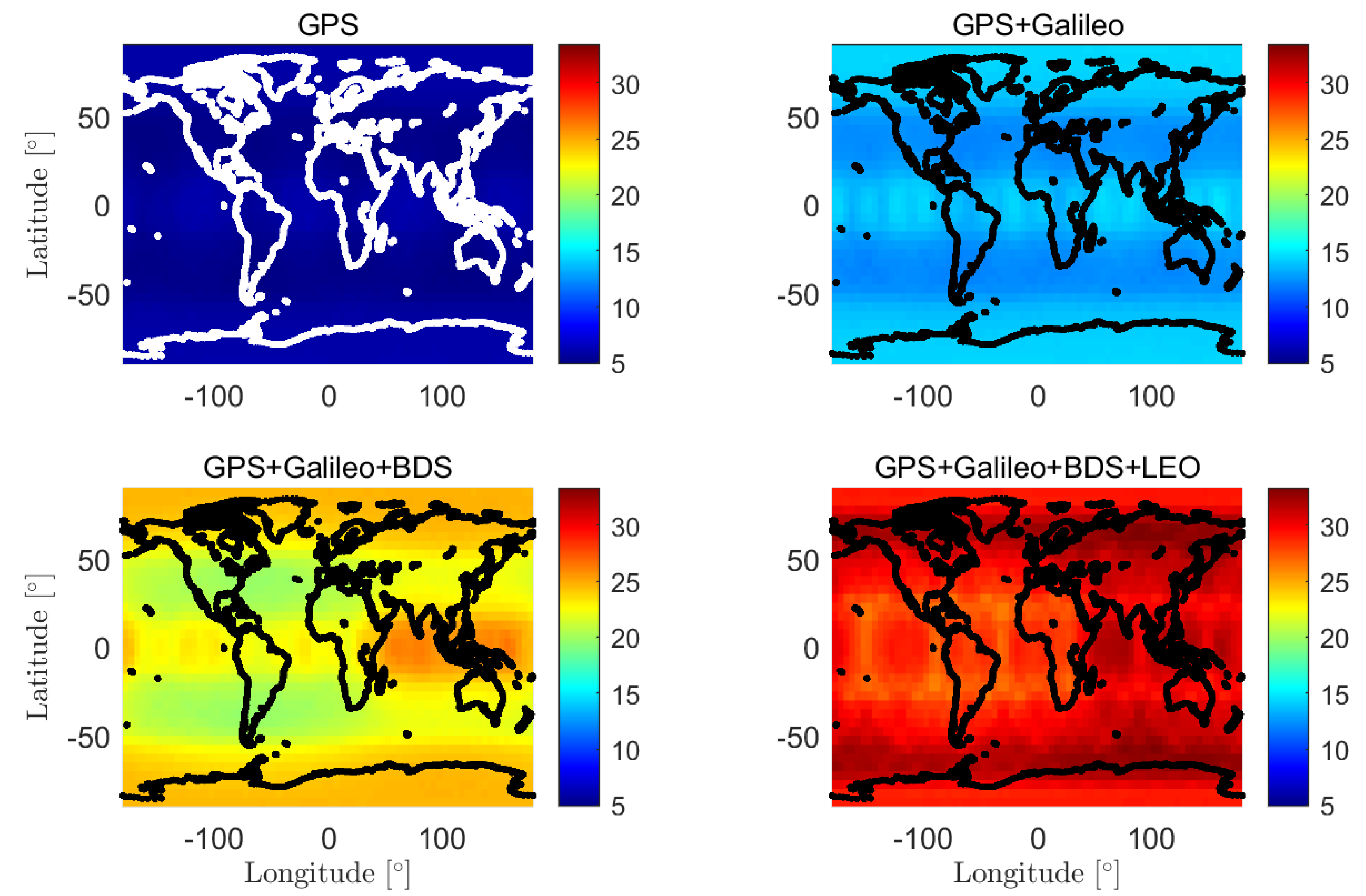
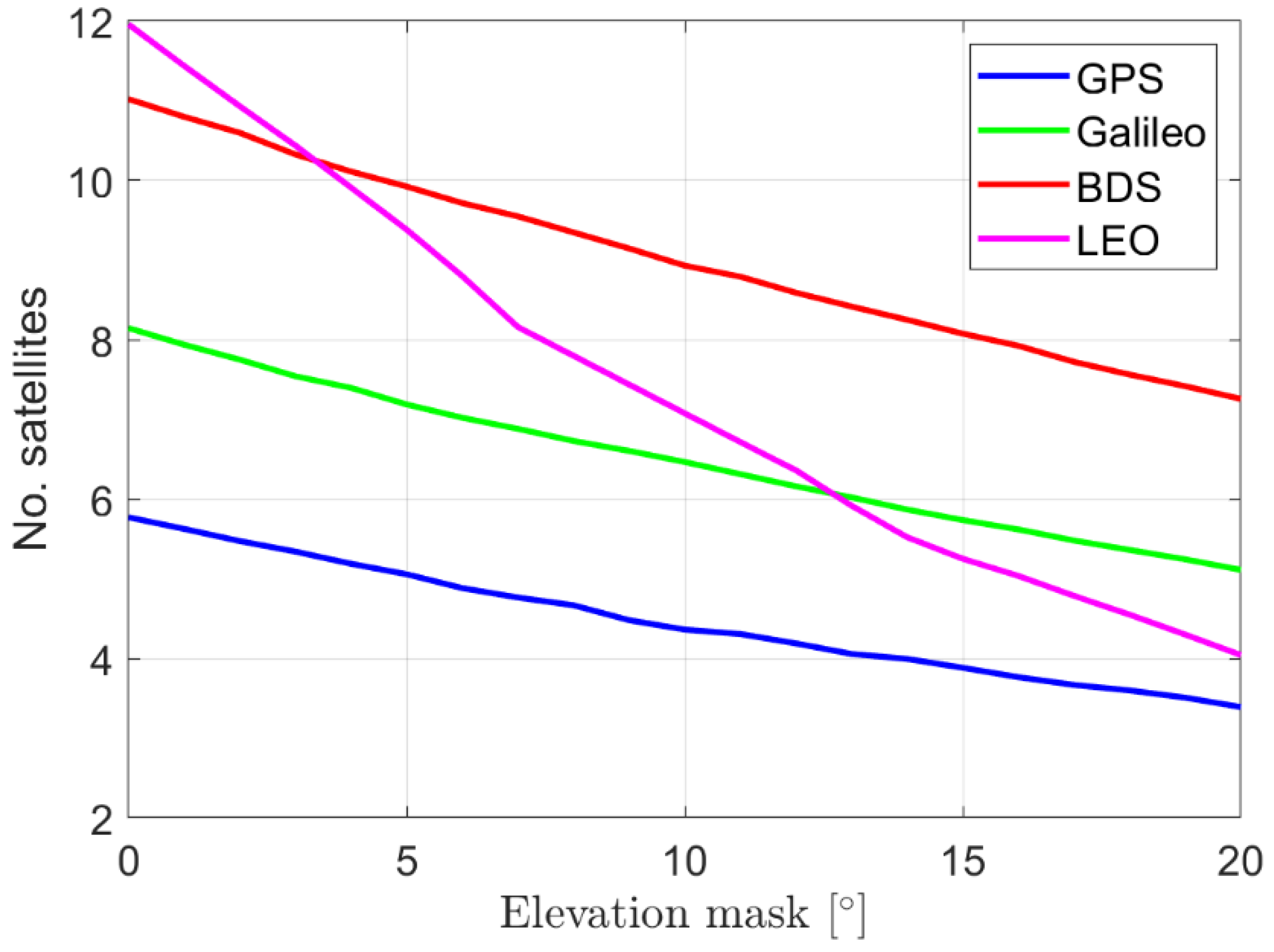
2.2. Satellite Numbers
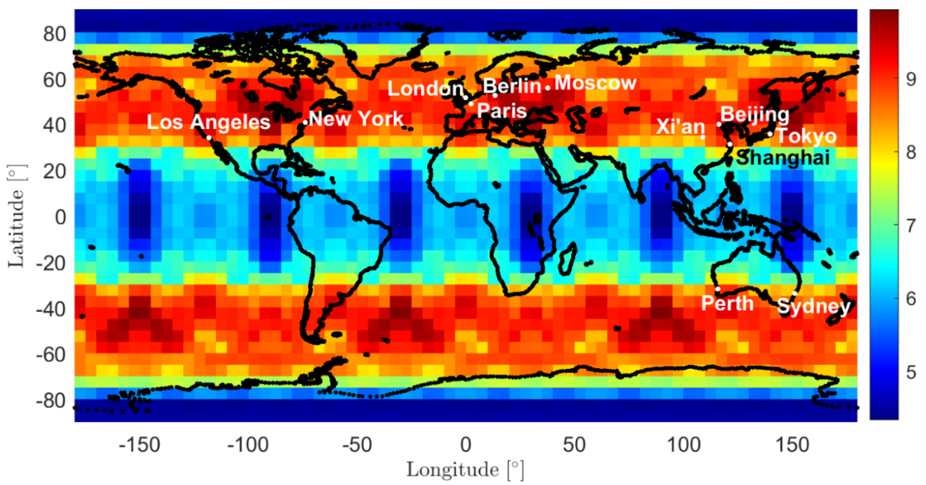
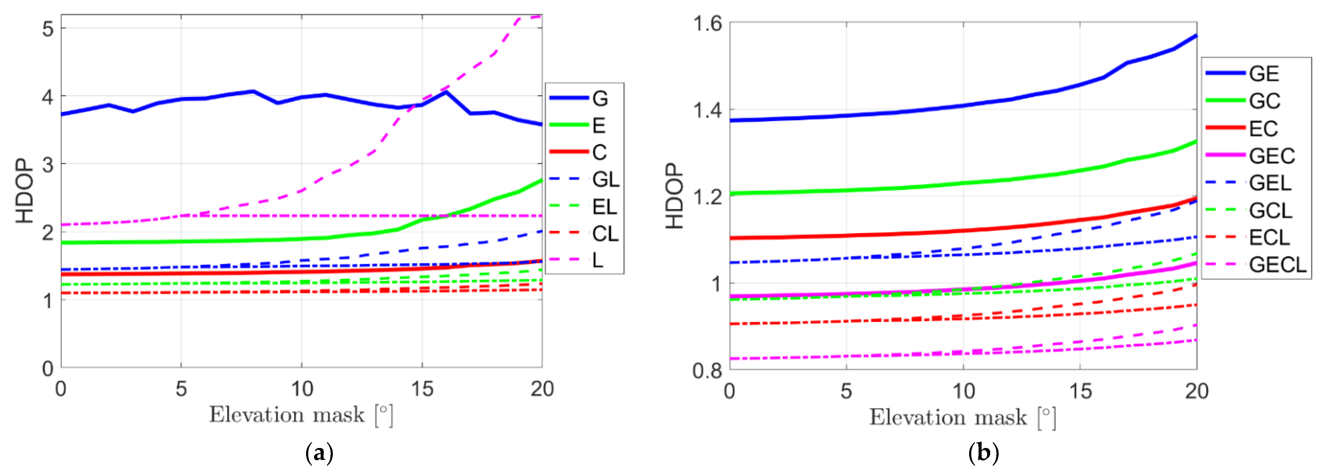
With more constellations contributing to the positioning service of the same user, the measurement geometry and the positioning precision can with no doubt be improved. Figure 3 are colormaps of the mean visible GNSS + LEO satellite numbers, transmitting signals on L1 and L5 frequencies, in 5 ° × 5 ° grids on a daily basis, calculated with a sampling interval of 10 min. The international GNSS service (IGS) [30] multi-GNSS experiment (MGEX) [31] orbits from the center for orbit determination in Europe (CODE) [32] on 26 June 2021, were used for the plots, which did not include the BDS GEO satellites. The elevation mask is set to 5 degrees. The LEO satellite configuration introduced in Section 2.1 is used for generation of the plots.
From Figure 3, it can be observed that adding the proposed LEO constellation (right-bottom subplot) has increased the visible satellite numbers to around or more than 30 in most places in the world. The distribution of the satellite numbers is generally latitude-dependent. Figure 4 illustrates in a colormap the number of simultaneously visible LEO satellites on a daily average basis with an elevation mask of 5 degrees. The latitude-related colors show that the proposed LEO constellation is especially beneficial to the mid-latitude areas. Several large cities are marked in the figure as examples. It can be observed that Moscow, Beijing, New York, Los Angeles and Berlin are all within the red areas, i.e., having more than nine satellites simultaneously visible on average.
The LEO satellites under the given configuration, however, are mostly visible at low elevation angles. Taking Beijing as an example, as shown in Figure 5, a much more rapid decrease can be observed in the LEO satellite numbers compared to other constellations when increasing the elevation mask. For an elevation cut-off angle of 10 degrees, the visible LEO satellite number is decreased to about 7. Still, it can be observed that for elevation masks smaller than 20 degrees, the number of visible LEO satellites is higher than that of the current L1/L5 GPS satellites.
The different nature of the LEO and GNSS signals do show advantages for LEO-augmented positioning in complicated measurement environments such as urban canyons. In such environments, GNSS signals under low elevation angles are partially blocked by high infrastructures around the receiver, leading to a limited visible area only for satellites of high elevation angles. The other tracked signals from low elevation angles are often disturbed by high multipath effects, which bias the results and are often screened out or strongly down-weighted in the positioning. All these are more or less equivalent to manually setting a high elevation mask in the processing. Benefiting from the much lower orbital altitude, the LEO signals occupy a much stronger signal strength than the GNSS signals, which helps the LEO signals penetrate obstacles and possibly enable even indoor positioning [7]. In addition, the fast speed of LEO satellites whitens the multipath effects around the user [6]. This indicates that the mis-modelled multipath effects in kinematic and complicated environments are likely to be categorized as measurement noise, which is usually done in actual GNSS-based positioning for simplicity, but actually incorrect. In such cases, low-elevation LEO signals might have large noise that needs to be properly down-weighted, but not mis-modeled biases that need to be strongly down-weighted or screened out in extreme cases. All these imply that in urban canyons or other environments with a limited sky view, a lower elevation mask can be set for LEO satellites.

2.3. HDOP

The position dilution of precision (PDOP) is a unitless indicator to assess the measurement geometry [33], where lower PDOP values correspond to better positioning precision. For road transport users, the horizontal dilution of precision (HDOP) is of higher interest and will be discussed in this section. In this contribution, the HDOP is calculated considering an elevation-dependent weighting function P = ( 1 + 10 × exp ( θ r s 10 ° ) ) 2 [34], where θ r s denotes the elevation angle from receiver r to satellite s in degrees. This elevation-dependent weight function is often used for the GNSS processing [35,36]. Figure 6 shows the daily mean HDOPs without (solid lines) and with the augmentation of LEO satellites (dashed lines) at Beijing. The indicator “G”, “E”, “C” and “L” represents the GPS, Galileo, BDS and the tested LEO constellation, respectively. High HDOPs larger than 20 are not considered by calculating the daily mean values. As the signals of LEO satellites have whitened multipath effects and could penetrate infrastructures (see the last paragraph of Section 2.2), HDOPs of one more option are illustrated with the dashed-dotted lines in Figure 6, i.e., the case assuming that the elevation cut-off angle for LEO satellites does not increase with the x-axis after 5 degrees, while the elevation mask angles for other constellations still increase after 5 degrees. The GPS-only HDOPs (see the solid blue line in Figure 6a) do not increase with the elevation mask after 10 degrees due to the increasing number of excluded epochs with low satellite numbers and high HDOPs.
From Figure 6, it can be observed that the improvements of the LEO augmentation to the GNSS-based HDOPs are significant. The improvement factors f HDOP are given for different elevation masks in Table 2, which are formulated as:
f HDOP = HDOP 0 HDOP L HDOP 0 ,
where HDOP 0 and HDOP L represent the HDOP without and with the LEO augmentation, respectively. From both Figure 6 and Table 2 it can be seen that the LEO augmentation improves the horizontal positional geometry for all the listed GNSS-based single-, dual- and triple-constellations by more than 10%, where the increase has reached around or more than 20% for the three single-constellation scenarios. In the cases where the GNSS satellites can only be effectively used with a high elevation cut-off angle (20 degrees for example) while the mask for LEO satellites remains a low value (5 degrees for example), the HDOP improvements can be further increased by more than 3% (see the values in Table 2 after the slash signs). Comparing the values for “GL”, “EL” and “CL” with the blue, green and red dashed-dotted lines in Figure 6a and those for dual-frequency HDOPs with solid lines in Figure 6b, it can be observed that the LEO-augmented single-constellation HDOPs can reach a similar level to the dual-constellation GNSS HDOPs, i.e., about 1 to 1.5. The same applies to the LEO-augmented dual-constellation HDOPs (see the blue, green and red dashed-dotted lines in Figure 6b), which are at a similar level to the triple-frequency GNSS HDOPs (see the solid magenta line in Figure 6b). This indicates that if one or two GNSS constellations are not available for the L1/L5 positioning, the suggested LEO constellation can take their role and make up for deficiencies caused by the weakened measurement geometry. In addition, as illustrated by the magenta dashed-dotted line in Figure 6a, it is possible to achieve an HDOP below 2.5 using only the LEO satellites when the elevation mask angle remains 5 degrees (or lower). This is at a similar level to the Galileo-only HDOPs (see the solid green line in Figure 6a).
It is worth mentioning that the improvements of the LEO augmentation in the measurement geometry are even more significant in the vertical direction than in the horizontal direction, which would be of interest to, for example, drone and hydrographic applications. When keeping the elevation cut-off angle at 5 degrees for the LEO satellites, the vertical dilution of precision (VDOP) reaches 20% to 40% for the dual- and triple-constellation cases at an elevation mask of 20 degrees (corresponding to the last column of Table 2). The corresponding improvements are around or above 40% for the three single-constellation cases.

3. PPP-RTK Processing Strategy

The strategy of PPP-RTK processing is introduced in the first part of this series of papers [14]. It uses undifferenced and uncombined observations [37], and forms new estimable parameters based on the S -system theory [38] to avoid rank deficiencies. The tested LEO satellites are designed for navigation purposes and are expected to broadcast GNSS-like phase and code signals on L1 and L5. As with the GNSS signals, they experience errors such as noise, tropospheric delays, clock biases, hardware biases and ambiguities. The LEO satellites are located at the altitudes of about 300 to 1500 km [39], which are within or above the ionosphere layer that is present from about 50 to 1000 km above the Earth’s surface. In our contribution, the altitudes of the tested LEO satellites are 975 and 1100 km (see Table 1). The LEO signals are thus assumed to go through the ionosphere and suffer from similar ionospheric delays as the GNSS satellite signals.
The observation equations for the network processing can be formulated as follows:
E ( Δ φ r , j s ( t i ) ) = ( g r s ( t i ) ) T Δ τ r ( t i ) + d t ˜ r ( t i ) d t ˜ s ( t i ) μ j ι ˜ r s ( t i ) + 𝛿 ˜ r , j ( t i ) 𝛿 ˜ , j s ( t i ) + 𝜆 j N ˜ r , j s ( t i )
E ( Δ p r , j s ( t i ) ) = ( g r s ( t i ) ) T Δ τ r ( t i ) + d t ˜ r ( t i ) d t ˜ s ( t i ) + μ j ι ˜ r s ( t i ) + d ˜ r , j ( t i ) d ˜ , j s ( t i ) ,
where Δ φ r , j s and Δ p r , j s indicate the phase and code observed-minus-computed (O-C) term, respectively. The superscript T denotes the matrix transposition. The g r s maps the zenith tropospheric delay (ZTD) Δ τ r from the vertical to the slant direction. λ j is the wavelength on frequency f i , and μ j = f 1 2 / f j 2 is the coefficient for the ionospheric delay on frequency f i . The forms of the estimable receiver ( d t ˜ r ) and satellite clocks ( d t ˜ s ), the estimable ionospheric delays on L1 ( ι ˜ r s ) and ambiguity ( N ˜ r , j s ), the phase ( δ ˜ r , j ) and code receiver hardware biases ( d ˜ r , j ), as well as their counterparts for the satellite ( δ ˜ , j s , d ˜ , j s ) are given in the first part of this series of papers (see Table 1 in [14]). E ( · ) is the expectation operator. Note that the d t ˜ r , δ ˜ r , j and d ˜ r , j are different for each constellation. The ZTDs, the hardware biases and the ambiguities are assumed linked in time by a random-walk noise.
With the partial ambiguity resolution (PAR) [40] enabled, the ambiguities are resolved using the least-squares ambiguity decorrelation adjustment (LAMBDA) method [41] for each constellation. A formal ambiguity success rate of 99.99% is set to be the threshold for successful ambiguity fixing, and a ratio test with a threshold of 3 is set for the ambiguity validation [42].
After the convergence of the network solutions, satellite clocks, satellite phase biases and ionospheric delays (of the network stations) are provided to users. To achieve fast integer ambiguity resolution (IAR) of the user, it is essential to interpolate the user ionospheric delays, e.g., based on the least-squares collocation [43] and the best linear unbiased prediction (BLUP) method [44]. In general, the interpolated user ionospheric delay vector ι ˜ ^ u ( t i ) can be expressed as:
ι ˜ ^ u ( t i ) = F ι u ( t i ) ( ι ˜ ^ ( t i ) d ^ u r , GF ( t 1 | i 1 ) ) ,
where ι ˜ ^ denotes the estimated ionospheric vector of all network stations and satellites, d ^ u r , GF ( t 1 | i 1 ) is the geometry-free (GF) code bias at t 1 between a reference network station u and the network station r , which is estimated during the ionosphere interpolation of the previous epoch. F ι u contains the interpolation coefficients for building the user ionospheric delays.
The estimated satellite clocks ( d t ˜ ^ s ), satellite phase biases ( δ ˜ ^ , j s ) and the interpolated user ionospheric delays ( ι ˜ ^ u s ) are corrected in the user observations with:
E ( Δ φ u , j s ( t i ) + d t ˜ ^ s ( t i ) + δ ˜ ^ , j s ( t i ) + μ j ι ˜ ^ u s ( t i ) ) = ( G s ( t i ) ) T Δ x u ( t i ) + ( g s ( t i ) ) T Δ τ u ( t i ) + d t ˜ ˜ u ( t i ) + δ ˜ ˜ u , j ( t i ) + λ j N ˜ u , j s ( t i ) ,
E ( Δ p u , j s ( t i ) + d t ˜ ^ s ( t i ) μ j ι ˜ ^ u s ( t i ) ) = ( G s ( t i ) ) T Δ x u ( t i ) + ( g s ( t i ) ) T Δ τ u ( t i ) + d t ˜ ˜ u ( t i ) + μ j d ˜ ˜ u , GF ( t i ) ,
where the estimable user receiver clock ( d t ˜ ˜ u ), user receiver phase bias ( δ ˜ ˜ u , j ) and GF code bias ( d ˜ ˜ u , GF ) vary for different constellations. Their forms can be found in [14]. G s denotes the satellite-to-receiver unit vectors, and Δ x u denotes the positional increments to the a priori values. In addition to the corrections themselves, the variance-covariance (V-C) matrices of the combined network corrections, i.e., d t ˜ ^ s ( t i ) + δ ˜ ^ , j s ( t i ) + μ j ι ˜ ^ u s ( t i ) for phase and d t ˜ ^ s ( t i ) μ j ι ˜ ^ u s ( t i ) for code, need to be considered in the user processing to enable fast and correct IAR. For converged network solutions, the variance due to the user ionosphere interpolation plays a major role in the V-C matrix of the combined network corrections.
With the combined network corrections and its V-C matrix computed, the user processing is performed with the PAR enabled using the same threshold for the ASR and the ratio test. More details of the PPP-RTK processing can be found in the first part of this series of papers [14].

4. LEO Augmentation

The first part of this series of papers [14] introduced the IM procedure of multi-GNSS PPP-RTK positioning. In this section, the differences in the positioning precision and the HPLs after the LEO augmentation will be discussed in detail. The GPS/Galileo/BDS-3 satellites transmitting signals on 1575.42 and 1176.45 MHz, i.e., L1/L5 for GPS, E1/E5a for Galileo and B1C/B2a for BDS-3 on 26 June 2021 are used for test simulations together with the considered LEO constellation. The elevation mask angle is set to 10 degrees for GNSS satellites and a lower value of 5 degrees for LEO satellites, assuming the user is not located in a high-density urban area. As shown in Figure 7, the same three networks with different sizes are used for simulations as in the first part of this series of papers (see Figure 2 in [14]), and the user at one of the worst locations for ionospheric interpolation is utilized for user processing in each network (see the stars in Figure 7, also see Figure 5 in [14]). Recall that the inter-station distance varies from 42 to 140 km in Network 1, from 101 to 337 km in Network 2 and from 168 to 563 km in Network 3.
Similar to the simulated GNSS observations in [14], the LEO observations are simulated taking into consideration the observation noise, the random-walk ZTDs, hardware biases, and spatially correlated ionospheric delays. The sampling interval of the data is set to 1 s. The standard deviations of different parameters for accuracy and continuity purposes are given in Table 4 of [14], and those for integrity purposes are given in Table 6 of [14].

4.1. Orbital Errors

Due to the high altitudes of the GNSS satellites, the influences of orbital errors on baselines of a few hundreds of kilometers can be neglected when using high-precision real-time orbits with an accuracy of centimeters. For LEO satellites which have much lower altitudes, i.e., from a few hundreds of kilometers to more than 1000 km, the influences of the orbital errors need to be analyzed when the distance between the network stations and the user reaches a few hundreds of kilometers.
The orbital errors in the radial ( δ R ), along-track ( δ S ) and cross-track directions ( δ W ) are projected into the signal direction to a network (r) and a user station (v), denoted as δ v and δ r , respectively. Their differences δ r v can be expressed as:
δ r v = δ v δ r = e R , e L v δ R + e S , e L v δ S + e W , e L v δ W e R , e L r δ R e S , e L r δ S e W , e L r δ W = ( e R , e L v e R , e L r ) δ R + ( e S , e L v e S , e L r ) δ S + ( e W , e L v e W , e L r ) δ W ,
where e R , e W and e S are the unit vectors in the radial, along-track and cross-track directions of the LEO satellite, respectively. e L v and e L r denote the unit vectors from the LEO satellite to the two stations. · , · forms scalar product of two vectors. When not considering the correlation among the orbital errors in the three directions, the standard deviation of δ r v , denoted as σ r v , is formulated using the variance law as:
σ r v = ( e R , e L v e R , e L r ) 2 σ R 2 + ( e S , e L v e S , e L r ) 2 σ S 2 + ( e W , e L v e W , e L r ) 2 σ W 2
for which σ R , σ S and σ W represent the standard deviation of the LEO satellite orbital errors in the radial, along-track and cross-track directions, respectively.
Considering the sizes of the three simulated networks as introduced in [14], as shown in Figure 7, with the inter-station distance ranging from about 40 to 560 km, the influences of the LEO orbital errors are investigated for baselines with one station located at the red star in Beijing (see Figure 8a), and the other station illustrated with blue dots having an latitude or longitude differences ranging from 0.5 to 5 degrees, i.e., with an inter-station distance ranging from about 43 to 555 km. The tested LEO constellation introduced in Section 2.1 is used for the analysis. The standard deviations of the orbital errors, i.e., σ R , σ S and σ W , are assumed to be 1 cm in each of the radial, along-track and cross-track directions for the reduced-dynamic precise orbit determination (POD), which normally exhibit an accuracy of centimeters using the post-processed GNSS products [45]. Note that using real-time GNSS products, the orbital accuracy of LEO satellites could be degraded depending on the products used [46].
Based on Equation (10), the daily averaged standard deviations of the orbital influences on different baselines are shown in Figure 8b. The blue and red dots represent the LEO orbits with an altitude of 975 and 1100 km, respectively (see Section 2.1). The daily averaged standard deviations are calculated as the square root of the averaged σ r v 2 for all satellites in the corresponding LEO layer and all epochs on the test day 26 June 2021, with a sampling interval of 1 min. From Figure 8b it can be observed that the σ r v is generally below 1 mm for the tested LEO constellation, even for baselines over 500 km. The influences of orbital errors are thus not further considered in this study. However, as shown by the lower values of the red dots than the blue dots, it is visible that the altitude of the LEO satellites plays an important role in the σ r v . For LEO satellites with lower altitudes, or for orbital products with significantly lower precision, the influences of the orbital errors need to be assessed for the corresponding situation, and if necessary, considered in the IM.

4.2. Network Processing

Before the user processing, the network corrections, i.e., the satellite clocks, satellite phase biases and ionospheric delays should be available from a network processing using L1/L5 observations from a four-constellation scenario (GPS/Galileo/BDS/LEO). The settings of the user processing are introduced at the beginning of Section 4.
In this contribution, the network corrections are assumed to be generated with all four constellations and with the PAR enabled. Compared with the three-constellation scenario of GPS/Galileo/BDS, the precision improvements are not significant in the combined network corrections when adding the LEO constellation, as new satellites mainly benefit the parameters that are commonly estimated for all constellations, i.e., the ZTDs in our case, but not the satellite-specific network corrections.
Recall that the considered LEO constellation broadcast code and carrier-phase observations that are interoperable with GNSS observations. With the PAR enabled for the four-constellation processing and with the ambiguities resolved constellation by constellation, as shown in Figure 9 for Network 1, the fix rate of the LEO satellite carrier-phase ambiguities that pass the success rate of 99.99% and get validated with the ratio test are shown to be lower than those of the other three GNSSs. This is related to the higher portion of the low elevation LEO satellites (see Figure 5). After the sharp increase within the first several minutes, the ambiguity fix rate of the LEO satellites remains at about 80% to 100%. This also applies to the Networks 2 and 3, which have larger sizes. Note that with the LAMBDA method, the ambiguities are first decorrelated with a transformation matrix before being resolved. The decorrelated ambiguities are thus linear combinations of the original ambiguities. With the decorrelated ambiguities successfully fixed to integers, they are transformed back to their original forms. As such, one unsolved decorrelated ambiguity could influence several ambiguities in their original forms. The fix rate shown in Figure 9 refers to the number of the fixed decorrelated ambiguities divided by the total number of the decorrelated ambiguities.

4.3. User Positioning

In this section, the focus is being put on the influences of the LEO augmentation on the user positioning results. The L1/L5 LEO signals are added to single-, dual- and triple-GNSS scenarios assuming that the user might not track all the three GNSS constellations. The user processing begins 60 s after the network processing to allow for the convergence of the network solutions. The settings of the user processing are introduced at the beginning of Section 4.

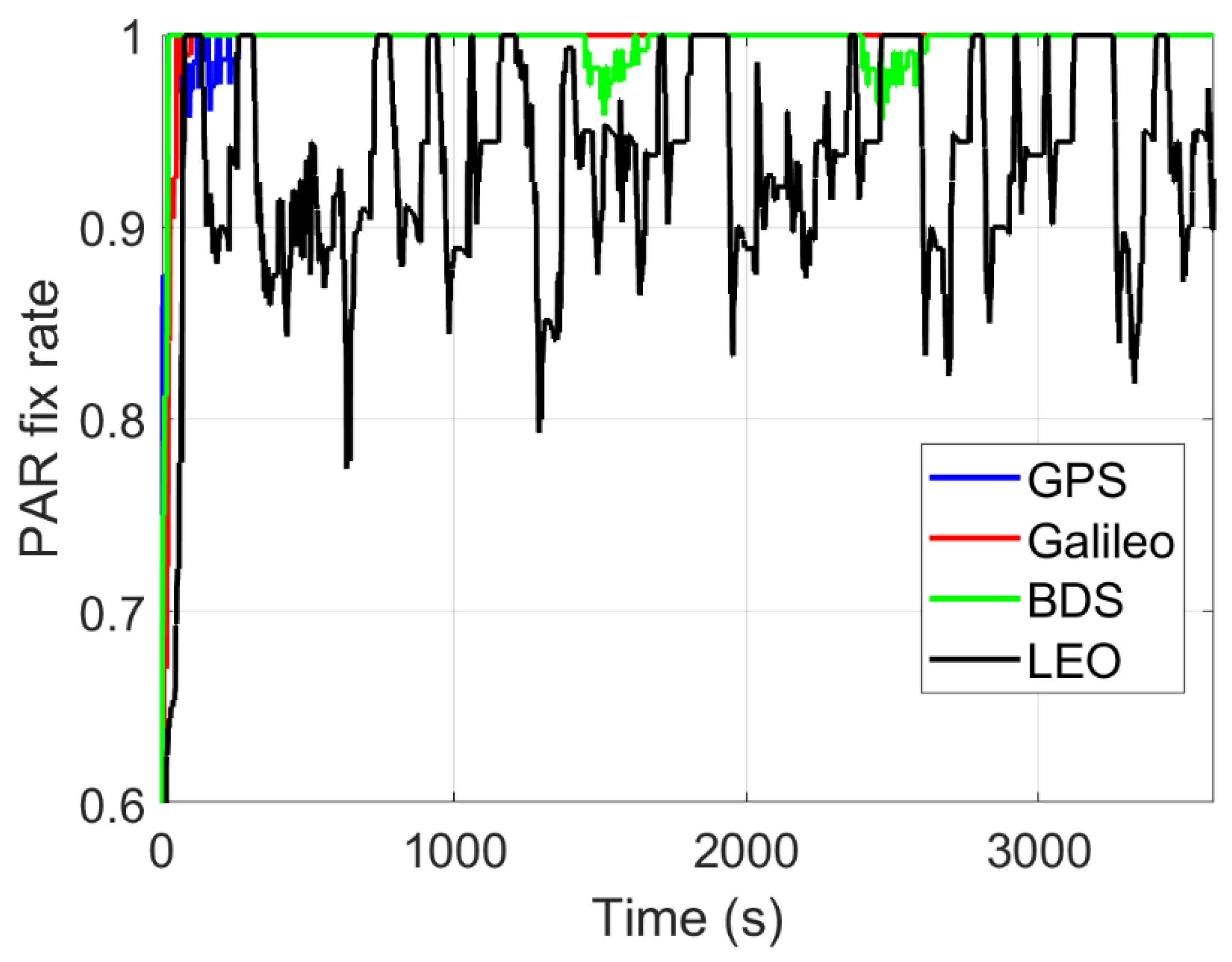
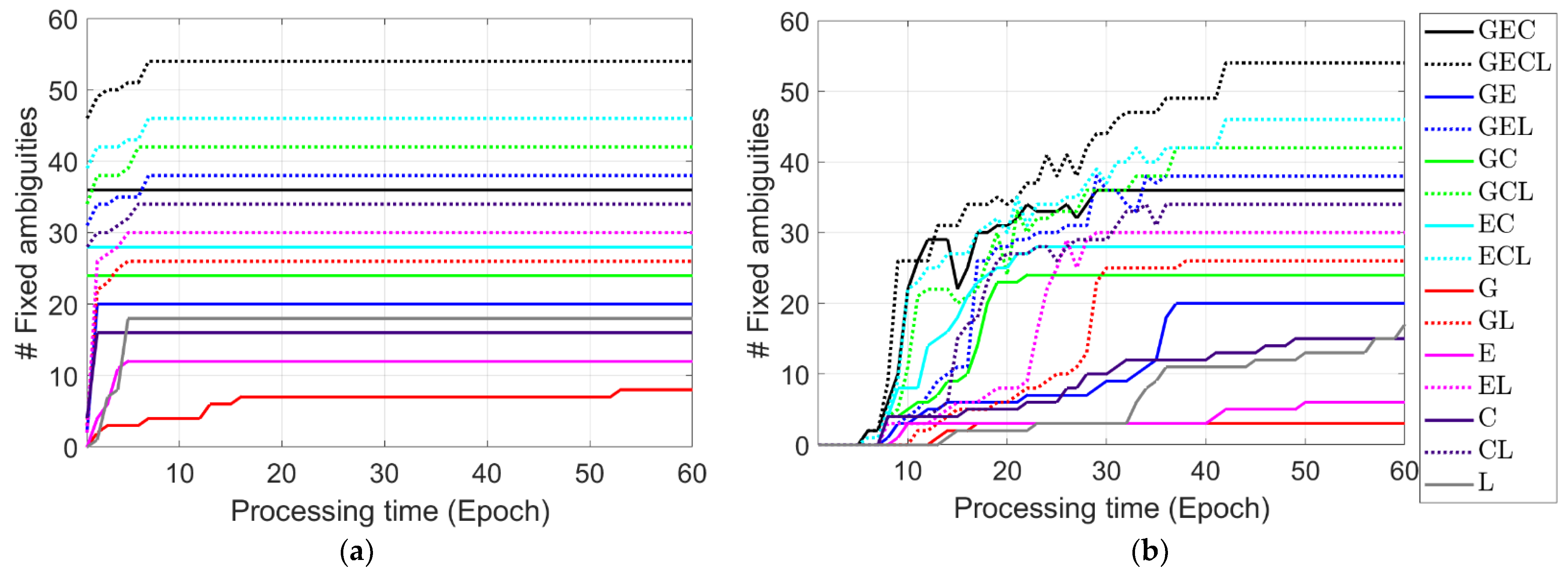
4.3.1. Ambiguity Resolution

The PAR is enabled at the user side with ambiguities from all constellations resolved together. Figure 10 illustrates the number of fixed decorrelated ambiguities in PAR for different constellation combinations at the user side. The dotted lines represent the cases with LEO augmentation. Note that the full ambiguity resolution (FAR) is achieved at the 60th epoch for all the lines in Figure 10a. The number of fixed ambiguities is shown in order to illustrate the fact that under LEO-augmentation, an increasing number of total ambiguities (see the ambiguity numbers reaching FAR at the 60th epoch in Figure 10a) does not hamper the speed of ambiguity resolution. Figure 10a corresponds to the case of using corrections from Network 1 with the smallest size among the three networks and under a relatively quiet ionospheric condition, i.e., with the standard deviation of the between-station ionospheric signals ( σ ι i j , 1 km ) set to 1.5 mm at 1 km. In such a case, the variance of the between-station combined network corrections tends to be small due to the precise ionospheric interpolation (see Figure 5 in [14]). The fix rate rises quickly to 1 in almost all cases except for the GPS-only scenario (see the solid red line in Figure 10a) due to the limited number of GPS satellites transmitting on L1/L5 at the moment and those observed by the user. From Figure 10a it can be observed that the total number of ambiguities has been significantly increased under the LEO augmentation (dotted lines), which does not slow down the ambiguity resolution. For single-constellation scenarios (see the red, magenta and dark purple lines) with limited satellite numbers, LEO augmentation has accelerated the ambiguity resolution due to the increased model strength.
In Figure 10b, network corrections are processed in Network 3 which has a larger size and under a more active ionospheric condition with σ ι i j , 1 km set to 5 mm. For the same constellation combinations, compared with Figure 10a, it is clear that a lower precision of the combined network corrections (at the between-satellite level) slows down the ambiguity resolution. However, under such a case, the benefits of the LEO augmentation become more evident for the single-constellation scenarios. Taking the GPS- and Galileo-only cases (see the red and magenta lines in Figure 10b) as examples, without LEO augmentation, the FAR is not reached until the 60th epoch, while adding the LEO constellation enables the FAR at about the 30th to the 40th epochs. From Figure 10 it can also be observed that the LEO-only scenario (see the gray lines) does not behave worse than the GPS- and Galileo-only scenarios for L1/L5 satellites. For user processing without the need to estimate satellite-specific parameters such as satellite clocks and phase biases, the rapid geometry change strengthens the model and accelerates the ambiguity resolution under the LEO augmentation. Recall that the elevation cut-off angle of LEO satellites was set to 5 degrees due to their stronger signal strength, while for GNSS satellites it is set to 10 degrees.
It is also noted that ambiguity resolution here is performed based on simulated data, which delivers formal results without consideration of the mis-modeled effects. The results aim to show the improvement in the efficiency of the ambiguity resolution when having the LEO augmentation. With mis-modeled effects, the number of resolved ambiguities could be reduced at the same processing time. As such, the positioning solutions and the HPLs are assessed in both the ambiguity-float and -fixed cases, for which the former case represents an extreme situation that no ambiguities are fixed.

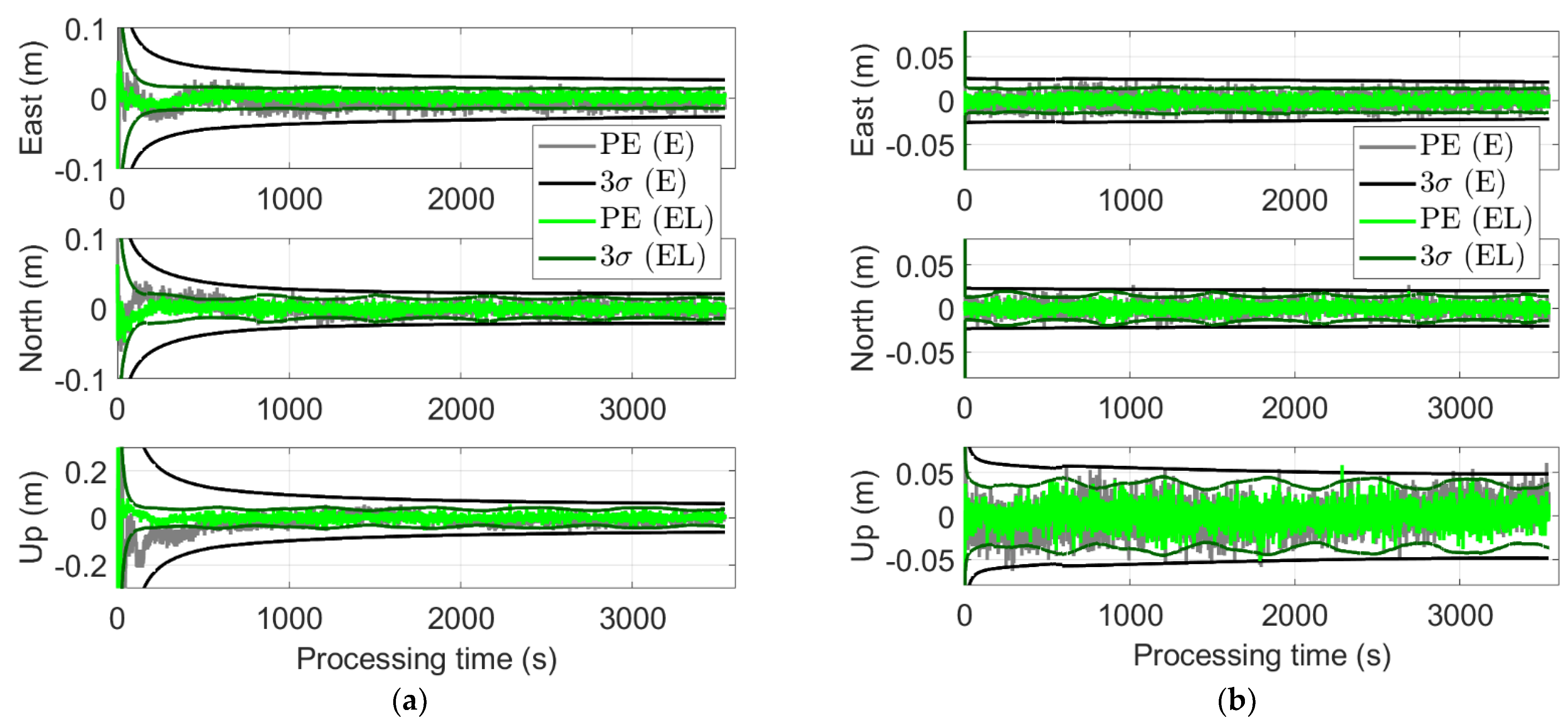
4.3.2. Positioning Results

The addition of LEO satellites also impacts the user positioning precision. As an example, Figure 11 shows the user positioning results based on the simulated data from Network 1 under quiet ionospheric conditions (with σ ι i j , 1 km set to 1.5 mm). The positioning errors in the Galileo-only scenario (see the gray lines) and the Galileo-LEO-scenario (see the light green lines) are generally bounded by their corresponding 3 σ -lines, in agreement with the 99.7% theoritical bounding (see the black and dark green lines). Reductions in the formal positional precision can be seen for both cases without and with the PAR enabled. This is especially obvious at the beginning phase of the ambiguity-float processing (see Figure 11a), where sharp convergence happens in the formal precision of the positioning.
When being augmented with the LEO constellation, the improvement in the formal horizontal precision, denoted as f H , is formulated as:
f H = σ N 0 2 + σ E 0 2 σ N 2 + σ E 2 σ N 0 2 + σ E 0 2
where σ N 0 and σ E 0 denotes the formal standard deviation of the north and the east positional component without the LEO augmentation, respectively. Their counterparts with the LEO augmentation are denoted by σ N and σ E .
Figure 12 shows the improvement ( f H ) in the formal horizontal precision by adding the LEO augmentation for Network 1 with a σ ι i j , 1 km of 1 mm (panel a) and for Network 3 with a σ ι i j , 1 km of 5 mm (panel b). The solid and dotted lines denote the cases with and without the PAR enabled, respectively. In general, the improvement is more significant in the ambiguity-float case, especially within the first 1000 epochs. For both the ambiguity-fixed and -float cases, the improvements for single-constellation scenarios, e.g., using low-cost receivers, are greater than those for dual- and triple-constellation scenarios. In general, the improvement in the formal horizontal precision amounts to about 10% to 40% after resolving the ambiguities, while it reaches about 40% to 70% for the ambiguity-float solutions within the first 1000 epochs.
For ambiguity-float solutions, the convergence time to a good precision is of great interest to users. Figure 13a shows the convergence time needed to let the formal horizontal precision reach 0.02 m in the ambiguity-float case, given here for demonstration purposes only for formal results, where typically 10 cm is sufficient for ambiguity-float real data when mis-modelled effects are considered. The two scenarios distinguish between high and low precision of the combined network corrections, i.e., from Network 1 with a σ ι i j , 1 km of 1.5 mm (Scenario 1) and from Network 3 with a σ ι i j , 1 km of 5 mm (Scenario 2). It can be observed that with the LEO augmentation, the convergence time is significantly shortened for all constellation combinations, especially for the single-constellation cases and for Scenario 2 (see the dark and light green bars). The convergence time is shortened to within 3 min for all cases, even under Scenario 2 (see the light green bars in Figure 13a). As shown in Table 3, the improvement has reached over 85% for the single-constellation scenarios under Scenario 2. Note that the results discussed here are the formal precision based purely on the model, aiming to show the impact of the strengthened model with LEO augmentation. Mis-modeled effects such as multipath or unmodelled ionospheric interpolation errors would bias the results and could further hamper the convergence. The shortened convergence time is related to the rapid change in geometry of the LEO satellites. For this aspect, it is similar to shortening the PPP convergence time with the LEO augmentation.
For the ambiguity-fixed solutions, the formal precision that could be reached after FAR shows the potential of the PPP-RTK positional performance. Figure 13b shows the formal horizontal precision after 1 h of the processing with the PAR enabled. With the LEO augmentation, the ambiguity-fixed horizontal precision is also improved due to the increased model strength. The formal horizontal precision at 1 h is reduced to within 1 cm for all constellation combinations and under both scenarios with LEO augmentation.

4.4. Horizontal Protection Level

The HPL is supposed to overbound the horizontal positioning errors (HPEs) under a pre-defined PMI H . The method to calculate the HPL was described in detail in the first part of this series of papers [14]. As mentioned in [14], the HPLs, while they depend on the observation quality and geometry, the nominal error model and the threat model, they are also affected by multipath environments, ionospheric activities, network size and PMI H . In this section, the same settings of the overbounding standard deviations and biases as in Table 6 of [14] will be used to evaluate the influences of the LEO augmentation on the HPLs. Recall that the multipath environments were distinguished into four categories (A, B, C and D) with the overbounding standard deviation for phase noise/multipath σ ˇ u 0 , φ varying from 0.005 to 0.02 m, and with the corresponding overbounding bias b ˇ u 0 , φ varying from 0.01 to 0.04 cycles. Their counterparts for code noise/multipath vary from 0.5 to 2 m for the overbounding standard deviation σ ˇ u 0 , p and from 0.2 to 0.8 m for the overboudning bias b ˇ u 0 , p . Simiarly, the ionospheric environments were distinguished into categories A, B, C and D, with the σ ˇ ι i j , 1 km varying from 5 to 20 mm. Details are described in Table 7 of [14]. In this contribution, the PMI H is set to 2 × 10 6 , the smallest value among the test values in the first part of this series of papers. Four different constellation combinations are tested for the HPLs without, and with, the LEO augmentation under the L1/L5 scenario, i.e., GPS-only (G), GPS/Galileo-combined (GE), GPS/BDS-combined (GC) and GPS/Galileo/BDS-combined (GEC).

4.4.1. Ambiguity-Float HPLs

The amibiguity-float HPLs converge with the processing time. As discussed in [14], the speed of convergence is correlated with both the multipath and the ionospheric conditions. In this sub-section, the influences of the LEO augmentation on the ambiguity-float HPLs are discussed for different scenarios and constellation combinations.
Figure 14 shows the ambiguity-float HPLs for network 1 under quiet multipath and ionospheric conditions (Category A), and for network 3 under active multipath and ionospheric conditions (Category D). It is noted that the convergence of the ambiguity-float HPLs is not only related to the satellite number, but also to their configurations, especially at the beginning phase. The increased overbounding variances of the interpolated ionospheric delays, which do not consider the elevation-dependence in this study, could degrade the positional components in the two horizontal directions with different propotions. In addition, the accumulated bias projects onto the two horizontal directions with an absolute projection matrix (see Equation (37) in [14]). This could also lead to different behaviors in the HPLs compared to the horizontal precision. As such, for Figure 14, the focus is intended to be put on the differences between the cases without and with the LEO augmentation, i.e., the solid and dashed lines in Figure 14.
From Figure 14 it can be observed that adding LEO satellites leads to a dramatic reduction in the HPLs. With the LEO augmentation, the improvements in the HPLs have reached more than 60% after convergence for the period of about 5 to 30 min, with the HPLs brought down to about 0.2 and 1 m at around 5 min after the processing start for the two tested scenarios. The HPLs for the two test scenarios are shown in Table 4 at different convergence times. The rapid convergence with LEO augmentation is not only caused by the increased satellite number, but is also a result of the rapid geometry change generated by the LEO satellites.

4.4.2. Ambiguity-Fixed HPLs

With the PAR enabled, the HPLs without and with the LEO augmentation are illustrated in Figure 15 for the two test scenarios as discussed in Section 4.4.1, i.e., for network 1 with quiet multipath and ionospheric conditions, and network 3 with active multipath and ionospheric conditions. The discontiniuties in Figure 15b are caused by the different number of resolved ambiguities.
From Figure 15, it can be observed that the ambiguity-fixed HPLs are generally reduced after adding the LEO augmentation. Figure 16 shows the improvements in the PAR-enabled HPLs after adding the LEO constellation. After reaching the FAR, the improvements generally vary from about 10% to 60%, depending on the constellations used and the measurement/ionospheric environments. It can be observed that the improvements are especially large for poor measurement geometry with the GPS-only scenario.

5. Conclusions

In recent years, the continuously increasing number of LEO satellites has motivated investigations of LEO-augmented GNSS positioning. While the PPP method has become a hot spot in this regard, PPP-RTK positioning and its IM procedure have been less discussed. Based on the IM procedure proposed for the PPP-RTK positioning in the first part of this series of papers, this contribution discusses the influences of LEO augmentation on the PPP-RTK horizontal positioning and its HPLs. A dual-frequency L1/L5 scenario is simulated for networks of different sizes around Beijing with the planned CentiSpace LEO constellation augmenting the GPS, Galileo and BDS constellations. The study distinguishes between different scenarios with quiet and active multipath ionospheric environments, evaluates the formal standard deviations of the positional solutions in both the ambiguity-float and -fixed cases, and compares their HPLs without and with the augmentation of the LEO satellites.
The influences of the LEO augmentation are not only reflected in the increased satellite numbers (especially at low elevation angles) and reduced HDOPs, but also in the improvement in the PPP-RTK positioning precision and HPLs. For the ambiguity-float solutions, LEO augmentation was found to be able to significantly shorten the convergence time of the formal horizontal precision. Under single-constellation scenarios and with a low precision of the ionospheric interpolation caused by, e.g., large network size or/and active ionospheric activities, the convergence time of the formal horizontal precision to 0.02 m has been reduced from more than 15 min to within 3 min. Similarly, the ambiguity-float HPLs are also significantly improved by adding the LEO constellation. The improvements in the HPLs have reached more than 60% after 5 to 30 min from commencement of processing. At 5 min, the HPLs are brought down from sub-meter to about 0.2 m for the tested scenario with simple multipath condition and high precision of the ionospheric interpolation, and from about 2.5 m to 1 m for the tested scenario with complicated multipath condition and low precision of the ionospheric interpolation.
With the PAR enabled, the LEO augmentation is found able to accelerate the ambiguity resolution, especially for single-constellation scenarios and for low precision of the ionospheric interpolation. After reaching the FAR, the ambiguity-fixed formal horizontal precision is generally reduced to within 1 cm with LEO augmentation for all constellation combinations tested in the study. The improvements in the ambiguity-fixed HPLs are mostly within 10% to 60%.
It needs to be mentioned that the results discussed in this contribution mainly rely on the changed measurement geometry after adding the tested LEO constellation, i.e., with the increased satellite numbers and their rapid geometry change. The influences of the LEO augmentation are illustrated with formal results based on the proposed IM model and the tested overbounding parameters. Different ionosphere interpolation strategies, IM procedures and overbounding parameters could lead to differences in the model and the formal results, and mis-modeled effects could lead to differences in the empirical results. In summary, this contribution intends to deliver the following qualitative findings under the given LEO constellation for L1/L5 GNSS-based PPP-RTK positioning:
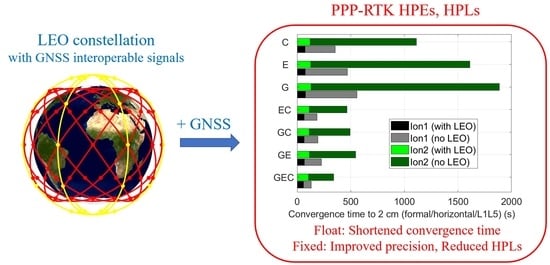
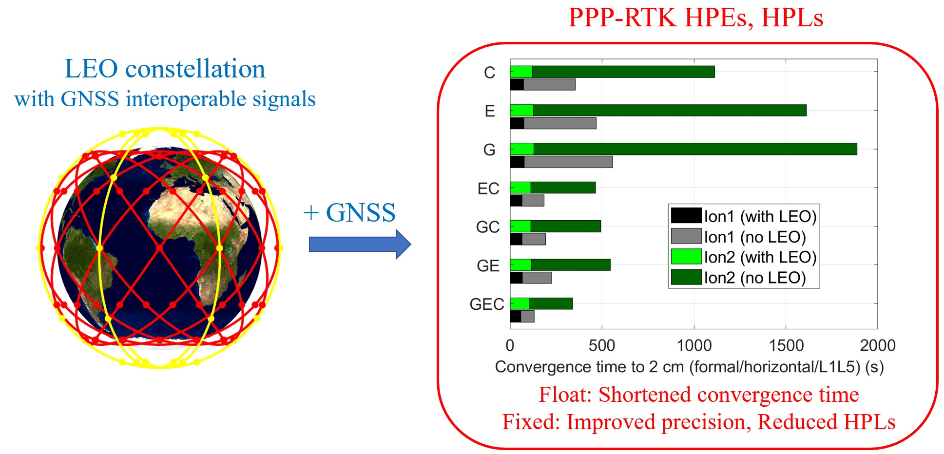
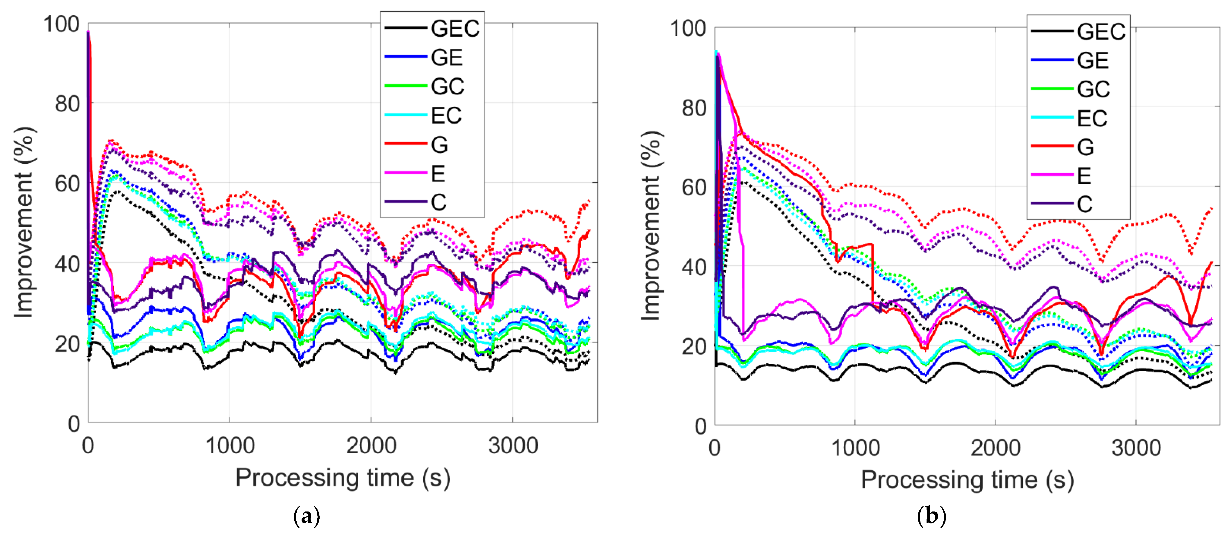
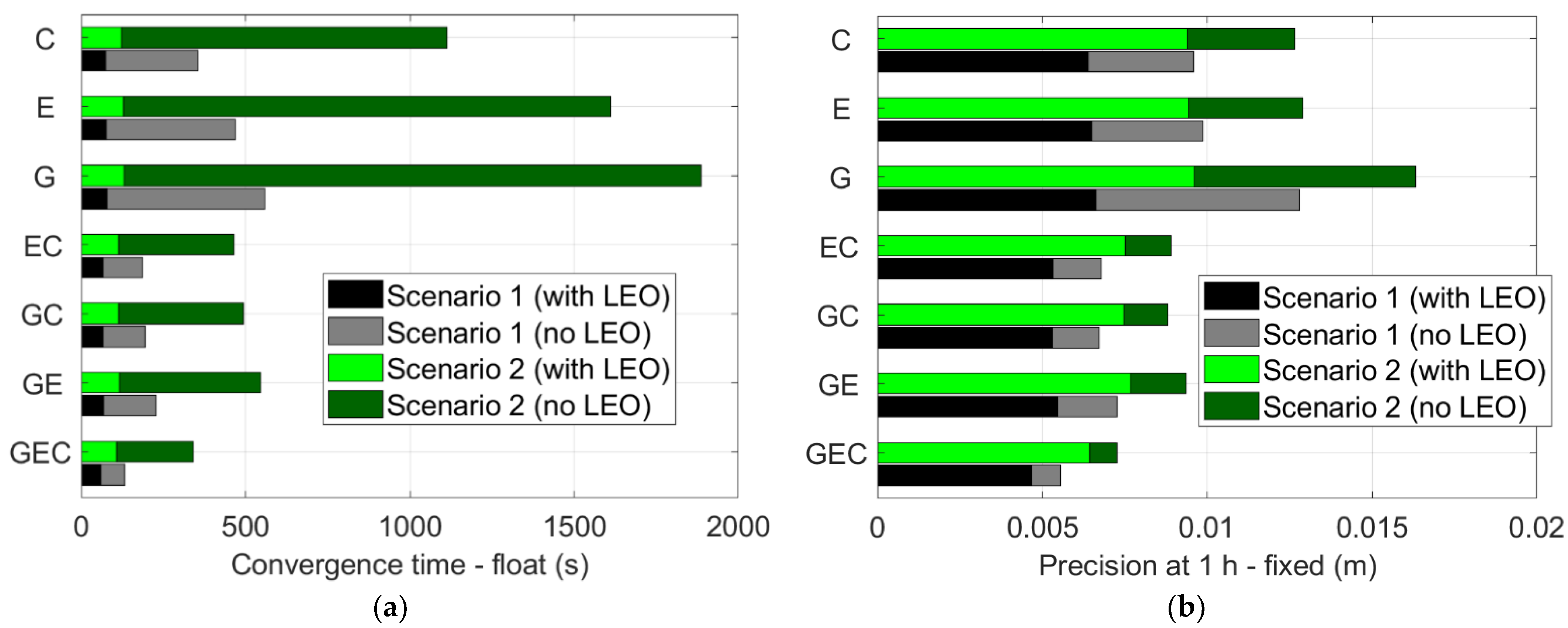
  • The convergence time of the ambiguity-float formal horizontal precision could be significantly reduced when augmenting GNSS by LEO measurements.
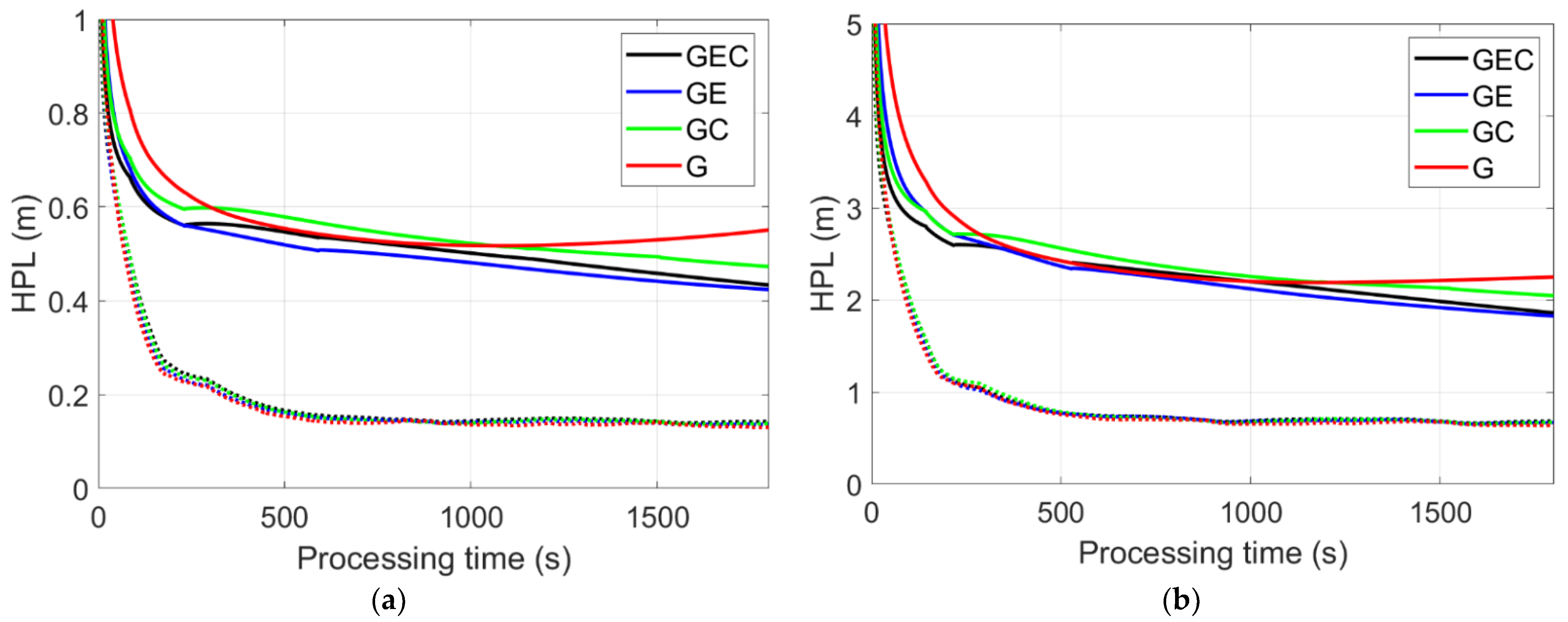
  • The ambiguity-float HPLs can be significantly reduced in the first half hour with the LEO augmentation.
  • The LEO augmentation accelerates the ambiguity resolution at the user side.
  • The LEO augmentation improves the ambiguity-fixed formal horizontal precision and reduces the ambiguity-fixed HPLs.
The above findings are expected to attract more attention in the field of the LEO-augmented PPP-RTK positioning, possibly with the overbounding parameters refined, with more efficient bias propagation strategies investigated and with real navigation signals from LEO satellites tested in the future.

Author Contributions

K.W. designed the work, processed the data and wrote the paper, W.W. contributed to the data acquisition, A.E.-M., L.Y. and X.Y. contributed to the revision of the paper. All authors have read and agreed to the published version of the manuscript.

Funding

This research is funded by the National Time Service Center, Chinese Academy of Sciences (CAS) (No. E167SC14), the CAS “Light of West China” Program (No. XAB2018YDYL01), the National Natural Science Foundation of China (No. 12073034), and the Australian Research Council—discovery project (No. DP 190102444) “Tracking Formation-Flying of Nanosatellites Using Inter-Satellite Links”.

Data Availability Statement

The multi-constellation precise orbital products are available at http://ftp.aiub.unibe.ch/CODE_MGEX/CODE (accessed on 21 March 2022).

Conflicts of Interest

The authors declare no conflict of interest.

References

  1. Reid, T.G.R.; Neish, A.M.; Walter, T.; Enge, P.K. Broadband LEO constellations for navigation. Navig. J. Inst. Navig. 2018, 65, 205–220. [Google Scholar] [CrossRef]
  2. Han, Y.; Wang, L.; Fu, W.; Zhou, H.; Li, T.; Xu, B.; Chen, R. LEO navigation augmentation constellation design with the multi-objective optimization approaches. Chin. J. Aeronaut. 2020, 34, 265–278. [Google Scholar] [CrossRef]
  3. Ge, H.; Li, B.; Ge, M.; Zang, N.; Nie, L.; Shen, Y.; Schuh, H. Initial assessment of precise point positioning with LEO enhanced global navigation satellite systems (LeGNSS). Remote Sens. 2018, 10, 984. [Google Scholar] [CrossRef] [Green Version]
  4. Li, X.; Ma, F.; Li, X.; Lv, H.; Bian, L.; Jiang, Z.; Zhang, X. LEO constellation-augmented multi-GNSS for rapid PPP convergence. J. Geod. 2018, 93, 749–764. [Google Scholar] [CrossRef]
  5. Li, M.; Xu, T.; Guan, M.; Gao, F.; Jiang, N. LEO-constellation-augmented multi-GNSS real-time PPP for rapid re-convergence in harsh environments. GPS Solut. 2022, 26, 29. [Google Scholar] [CrossRef]
  6. Faragher, R.; Ziebart, M. OneWeb LEO PNT: Progress or Risky Gamble? Inside GNSS. 28 September 2020. Available online: https://insidegnss.com/oneweb-leo-pnt-progress-or-risky-gamble/ (accessed on 28 June 2021).
  7. Lawrence, D.; Cobb, H.S.; Gutt, G.; O’Connor, M.; Reid, T.G.R.; Walter, T.; Whelan, D. Innovation: Navigation from LEO. GPS World. 30 June 2017. Available online: https://www.gpsworld.com/innovation-navigation-from-leo/ (accessed on 27 March 2021).
  8. Perez, R. Introduction to Satellite Systems and Personal Wireless Communications. In Wireless Communications Design Handbook; Volume 1: Space Inteference; Academic Press: Cambridge, MA, USA, 1998; pp. 1–30. [Google Scholar] [CrossRef]
  9. Cakaj, S.; Kamo, B.; Lala, A.; Rakipi, A. The Coverage Analysis for Low Earth Orbiting Satellites at Low Elevation. Int. J. Adv. Comput. Sci. Appl. 2014, 5, 6. [Google Scholar] [CrossRef] [Green Version]
  10. Jia, Y.; Bian, L.; Cao, Y.; Meng, Y.; Zhang, L. Design and Analysis of Beidou Global Integrity System Based on LEO Augmentation. In China Satellite Navigation Conference (CSNC) 2020 Proceedings: Volume II. CSNC 2020; Sun, J., Yang, C., Xie, J., Eds.; Lecture Notes in Electrical Engineering; Springer: Singapore, 2020; Volume 651, pp. 624–633. [Google Scholar] [CrossRef]
  11. Wang, K.; El-Mowafy, A.; Rizos, C. Integrity monitoring for precise orbit determination of LEO satellites. GPS Solut. 2021, 26, 32. [Google Scholar] [CrossRef]
  12. Wübbena, G.; Schmitz, M.; Bagge, A. PPP-RTK: Precise point positioning using state-space representation in RTK networks. In Proceedings of the ION GNSS 2005, Long Beach, CA, USA, 13–16 September 2005; pp. 2584–2594. [Google Scholar]
  13. Teunissen, P.J.G.; Khodabandeh, A. Review and principles of PPP-RTK methods. J. Geod. 2015, 89, 217–240. [Google Scholar] [CrossRef]
  14. Wang, K.; El-Mowafy, A.; Qin, W.; Yang, X. Integrity Monitoring of PPP-RTK positioning; Part I: GNSS-based IM procedure. Remote Sens. 2022, 14, 44. [Google Scholar] [CrossRef]
  15. Yang, L. The Centispace-1: A LEO Satellite-Based Augmentation System. In Proceedings of the 14th Meeting of the International Committee on Global Navigation Satellite Systems, Bengaluru, India, 8–13 December 2019. [Google Scholar]
  16. GPS Constellation Status for 02/01/2022. Available online: https://www.navcen.uscg.gov/?Do=constellationStatus (accessed on 1 February 2021).
  17. ICD. Beidou Navigation Satellite System. Available online: http://en.beidou.gov.cn/SYSTEMS/ICD/ (accessed on 1 February 2022).
  18. Nadarajah, N.; Khodabandeh, A.; Teunissen, P.J.G. Assessing the IRNSS L5-signal in combination with GPS, Galileo, and QZSS L5/E5a-signals for positioning and navigation. GPS Solut. 2016, 20, 289–297. [Google Scholar] [CrossRef]
  19. Choy, S.; Kuckartz, J.; Dempster, A.G.; Rizos, C.; Higgins, M. GNSS satellite-based augmentation systems for Australia. GPS Solut. 2017, 21, 835–848. [Google Scholar] [CrossRef]
  20. EU-U.S. Cooperation on Satellite Navigation, Working Group C—ARAIM Technical Subgroup. In Milestone 3 Report; Final Version; 25 February 2016. Available online: https://www.gps.gov/policy/cooperation/europe/2016/working-group-c/ARAIM-milestone-3-report.pdf (accessed on 21 March 2022).
  21. Blanch, J.; Walter, T.; Enge, P.; Lee, Y.; Pervan, B.; Rippl, M.; Spletter, A. Advanced RAIM user algorithm description: Integrity support message processing, fault detection, exclusion, and protection level calculation. In Proceedings of the ION GNSS 2012, Nashville, TN, USA, 17–21 September 2012; pp. 2828–2849. [Google Scholar]
  22. ED-259; Minimum Operational Performance Standard for Galileo/Global Positioning System/Satellite-Based Augmentation System Airborne Equipment. The European Organisation for Civil Aviation Equipment (EUROCAE): Saint-Denis, France, 2019.
  23. Wu, J.; Wang, K.; El-Mowafy, A. Preliminary performance analysis of a prototype DFMC SBAS service over Australia and Asia-Pacific. Adv. Space Res. 2020, 66, 1329–1341. [Google Scholar] [CrossRef]
  24. Michalak, G.; Glaser, S.; Neumayer, K.H.; König, R. Precise orbit and Earth parameter determination supported by LEO satellites, inter-satellite links and synchronized clocks of a future GNSS. Adv. Space Res. 2021, 12, 4753–4782. [Google Scholar] [CrossRef]
  25. Guenter, W.H. Status, perspectives and trends of satellite navigation. Satell. Navig. 2020, 1, 22. [Google Scholar] [CrossRef]
  26. Yuan, J.; Zhou, S.; Hu, X.; Yang, L.; Cao, J.; Li, K.; Liao, M. Impact of Attitude Model, Phase Wind-Up and Phase Center Variation on Precise Orbit and Clock Offset Determination of GRACE-FO and CentiSpace-1. Remote Sens. 2021, 13, 2636. [Google Scholar] [CrossRef]
  27. Walker, J.G. Satellite constellations. J. Br. Interplanet. Soc. 1984, 37, 559–571. [Google Scholar]
  28. SNL Online. List of Space Networks/Earth Stations (by Frequency and Orbital Position). International Telecommunication Union. Available online: https://www.itu.int/snl/freqtab_snl.html (accessed on 25 January 2022).
  29. Guan, M.; Xu, T.; Gao, F.; Nie, W.; Yang, H. Optimal Walker Constellation Design of LEO-Based Global Navigation and Augmentation System. Remote Sens. 2020, 12, 1845. [Google Scholar] [CrossRef]
  30. Johnston, G.; Riddell, A.; Hausler, G. The International GNSS Service. In Springer Handbook of Global Navigation Satellite Systems, 1st ed.; Teunissen, P.J.G., Montenbruck, O., Eds.; Springer International Publishing: Cham, Switzerland, 2017; pp. 967–982. [Google Scholar] [CrossRef]
  31. Montenbruck, O.; Steigenberger, P.; Prange, L.; Deng, Z.; Zhao, Q.; Perosanz, F.; Romero, I.; Noll, C.; Stürze, A.; Weber, G.; et al. The Multi-GNSS Experiment (MGEX) of the International GNSS Service (IGS)—Achievements, prospects and challenges. Adv. Space Res. 2017, 59, 1671–1697. [Google Scholar] [CrossRef]
  32. Dach, R.; Brockmann, E.; Schaer, S.; Beutler, G.; Meindl, M.; Prange, L.; Bock, H.; Jäggi, A.; Ostini, L. GNSS processing at CODE: Status report. J. Geod. 2009, 83, 353–365. [Google Scholar] [CrossRef] [Green Version]
  33. Langley, R.B. Dilution of precision. GPS World 1999, 10, 52–59. [Google Scholar]
  34. Euler, H.J.; Goad, C.C. On optimal filtering of GPS dual frequency observations without using orbit information. Bull. Geod. 1991, 65, 130–143. [Google Scholar] [CrossRef]
  35. Teunissen, P.J.G.; de Bakker, P.F. Next generation GNSS single receiver cycle slip reliability. In VII Hotine-Marussi Symposium on Mathematical Geodesy; International Association of Geodesy Symposia; Springer: Berlin/Heidelberg, Germany, 2012; Volume 137. [Google Scholar]
  36. El-Mowafy, A. Estimation of multi-constellation GNSS observation stochastic properties using single receiver single satellite data validation method. Surv. Rev. 2015, 47, 99–108. [Google Scholar] [CrossRef] [Green Version]
  37. Odijk, D.; Zhang, B.; Khodabandeh, A.; Odolinkski, R.; Teunissen, P.J.G. On the estimability of parameters in undifferenced, uncombined GNSS network and PPP-RTK user models by means of S-system theory. J. Geod. 2015, 90, 15–44. [Google Scholar] [CrossRef]
  38. Baarda, W. S-transformations and criterion matrices. In Publications on Geodesy, 2nd ed.; Netherlands Geodetic Commission: Delft, The Netherlands, 1981; Volume 5, No. 1. [Google Scholar]
  39. Montenbruck, O.; Gill, E. Around the world in a hundred minutes. In Satellite Orbits, 1st ed.; Springer: Berlin/Heidelberg, Germany, 2000; pp. 1–13. [Google Scholar]
  40. Nardo, A.; Li, B.; Teunissen, P.J.G. Partial Ambiguity Resolution for Ground and Space-Based Applications in a GPS + Galileo scenario: A simulation study. Adv. Space Res. 2016, 57, 30–45. [Google Scholar] [CrossRef]
  41. Teunissen, P.J.G. The least-squares ambiguity decorrelation adjustment: A method for fast GPS integer ambiguity estimation. J. Geod. 1995, 70, 65–82. [Google Scholar] [CrossRef]
  42. Teunissen, P.J.G.; Verhagen, S. On the Foundation of the Popular Ratio Test for GNSS Ambiguity Resolution. In Proceedings of the ION GNSS 2004, Long Beach, CA, USA, 21–24 September 2004; pp. 2529–2540. [Google Scholar]
  43. Moritz, H. Least-squares collocation. Rev. Geophys. 1978, 16, 421–430. [Google Scholar] [CrossRef]
  44. Teunissen, P.J.G.; Khodabandeh, A. BLUE, BLUP and the Kalman filter: Some new results. J. Geod. 2013, 87, 461–473. [Google Scholar] [CrossRef]
  45. Li, K.; Zhou, X.; Guo, N.; Zhao, G.; Xu, K.; Lei, W. Comparison of precise orbit determination methods of zero-difference kinematic, dynamic and reduced-dynamic of GRACE—A satellite using SHORDE software. J. Appl. Geod. 2017, 11, 157–165. [Google Scholar] [CrossRef]
  46. Allahvirdi-Zadeh, A.; Wang, K.; El-Mowafy, A. POD of small LEO satellites based on precise real-time MADOCA and SBAS-aided PPP corrections. GPS Solut. 2021, 25, 31. [Google Scholar] [CrossRef]
Figure 1. Frequency structure of the GPS, Galileo and BDS. The satellite numbers of different constellations/generations were retrieved on 1 February 2022.
Remotesensing 14 01599 g001
Figure 2. The tested LEO constellation (see Table 1) around the Earth. The red and yellow lines represent layers A and B, respectively.
Remotesensing 14 01599 g002
Figure 3. Colormaps of the daily mean numbers of satellites transmitting signals on L1 and L5.
Remotesensing 14 01599 g003
Figure 4. Daily averaged number of the simultaneously visible satellites of the tested LEO constellation.
Remotesensing 14 01599 g004
Figure 5. The daily average number of visible L1/L5 satellites of different constellations in Beijing under different elevation masks. The average number of satellites at an elevation mask angle of 5 degrees amounts to about 5.1, 7.2, 9.9, and 9.4 for GPS, Galileo, BDS and LEO satellites sending signals on L1/L5, respectively.
Remotesensing 14 01599 g005
Figure 6. Daily mean HDOPs using L1/L5 satellites from (a) single GNSS constellation; (b) dual and triple GNSS constellations, without and with the augmentation of LEO satellites. The dashed and dashed-dotted line represents the case that the elevation mask for LEO satellites increases and does not increase after 5 degrees, respectively.
Remotesensing 14 01599 g006
Figure 7. Networks of different sizes that are used for the network positioning. The stars represent the worst-location users in the three networks, which are used for the test results in user positioning and IM in Section 4.3 and Section 4.4.
Remotesensing 14 01599 g007
Figure 8. (a) Location of assumed baselines; (b) Daily averaged standard deviations of the orbital influences on the baselines, i.e., σ r v (Equation (10)). The standard deviations of the orbital errors are assumed to be 1 cm in the radial, along-track and cross-track directions each.
Remotesensing 14 01599 g008
Figure 9. Fix rate of the partial ambiguity resolution (PAR) for four-constellation processing using simulated data from Network 1. The different colors denote the constellation-wise PAR fix rate.
Remotesensing 14 01599 g009
Figure 10. Total number of fixed (decorrelated) ambiguities for different constellation combinations using: (a) Network 1 with a σ ι i j , 1 km of 1 mm; (b) Network 3 with a σ ι i j , 1 km of 5 mm. “#” means the number.
Remotesensing 14 01599 g010
Figure 11. User positioning results (based on simulations) and three times the formal standard deviations (3 σ ) of the positional components using Galileo (and LEO) satellites from Network 1 with σ ι i j , 1 km set to 1.5 mm in (a) the ambiguity-float case and (b) with the PAR enabled.
Remotesensing 14 01599 g011
Figure 12. Improvement ( f H ) of the formal horizontal precision by adding the LEO augmentation with (solid lines) and without the PAR enabled (dotted lines). The simulated data from (a) Network 1 with a σ ι i j , 1 km of 1 mm and (b) Network 3 with a σ ι i j , 1 km of 5 mm are used.
Remotesensing 14 01599 g012
Figure 13. (a) Convergence time of the ambiguity-float formal horizontal precision ( 1 σ ) to 0.02 m; (b) Ambiguity-fixed formal horizontal precision at 1 h. Scenario 1 and 2 denotes the network corrections from Network 1 with a σ ι i j , 1 km of 1.5 mm and from Network 3 with a σ ι i j , 1 km of 5 mm, respectively.
Remotesensing 14 01599 g013
Figure 14. Ambiguity-float HPLs without and with LEO augmentation for: (a) Network 1 under quiet multipath and ionospheric conditions (Category A); (b) Network 3 under active multipath and ionospheric conditions (Category D). The solid lines refer to the case without LEO, and the dotted lines represent the HPLs with LEO augmentation. Note that the y-scales are different in the two sub-figures.
Remotesensing 14 01599 g014
Figure 15. PAR-enabled HPLs without and with the LEO augmentation for (a) Network 1 under quiet multipath and ionospheric conditions (Category A); (b) Network 3 under active multipath and ionospheric conditions (Category D). The solid lines refer to the case without LEO augmentation, and the dotted lines represent the HPLs with LEO augmentation. Note that the y-scales are different in the two sub-figures.
Remotesensing 14 01599 g015
Figure 16. Improvements of the PAR-enabled HPLs by adding the LEO augmentation for (a) Network 1 under quiet multipath and ionospheric conditions (Category A); (b) Network 3 under active multipath and ionospheric conditions (Category D). Note that the y-scales are different in the two sub-figures.
Remotesensing 14 01599 g016
Table 1. Details of the tested LEO satellite constellation. H is the orbital height. N and P denotes the number of satellites and orbital planes in the corresponding layer, respectively. F describes the phase shift between adjacent planes, and I denotes the inclination.
Layer H [km] N P F I [°]
A97512012055
B1100303087.4
Table 2. Improvement factors in HDOPs using L1/L5 satellites from different GNSS constellations and under different elevation mask angles. The slash sign separates the cases that the elevation mask for LEO satellites increases and does not further increase after 5 degrees.
Constellation Improvement   Factor   f HDOP
10°15°20°
G62.6%60.4%/62.4%54.5%/60.8%43.8%/56.3%
E33.2%33.0%/34.2%38.7%/42.0%47.9%/53.3%
C20.1%19.9%/21.0%19.6%/22.8%21.4%/27.0%
GE23.7%23.4%/24.4%23.0%/25.9%24.3%/29.6%
GC20.1%19.9%/20.7%19.3%/21.6%19.5%/23.9%
EC17.8%17.4%/18.1%16.9%/18.9%16.7%/20.5%
GEC14.7%14.5%/15.0%13.9%/15.6%13.6%/17.0%
Table 3. Improvement of the convergence time to 0.02 m for the ambiguity-float formal horizontal precision, when adding the LEO constellation.
ScenarioGEC(L)GE(L)GC(L)EC(L)G(L)E(L)C(L)
154.2%69.9%65.8%64.9%86.2%83.8%79.4%
268.8%78.9%77.3%75.9%93.2%92.1%89.1%
Table 4. Ambiguity-float HPLs at different convergence times. The HPLs without and with LEO augmentation are separated by the slash signs.
ConstellationHPL (m)
30 s60 s180 s300 s1200 s
Network 1, quiet multipath and ionospheric condition (Category A)
G1.10/0.750.89/0.550.67/0.250.60/0.210.52/0.14
GE0.88/0.720.74/0.560.58/0.260.55/0.220.46/0.14
GC0.86/0.740.74/0.590.61/0.260.60/0.230.51/0.15
GEC0.79/0.710.70/0.580.58/0.270.56/0.230.49/0.15
Network 3, active multipath and ionospheric condition (Category D)
G5.42/3.474.27/2.573.06/1.182.69/1.012.19/0.67
GE4.32/3.413.56/2.642.81/1.212.61/0.992.03/0.69
GC3.95/3.363.35/2.672.81/1.262.71/1.072.19/0.71
GEC3.63/3.223.14/2.602.68/1.262.59/1.022.12/0.71
Publisher’s Note: MDPI stays neutral with regard to jurisdictional claims in published maps and institutional affiliations.

