Real-Time LEO Satellite Orbits Based on Batch Least-Squares Orbit Determination with Short-Term Orbit Prediction

Abstract

The augmentation of the Global Navigation Satellite System (GNSS) by Low Earth Orbit (LEO) satellites is proposed as an effective method to improve the precision and shorten the convergence time of Precise Point Positioning (PPP). Serving as navigation satellites in the future, LEO satellites need to be provided with their high-accuracy orbits in real-time. This would potentially enable the high-accuracy real-time LEO satellite clock determination, and eventually facilitate the high-accuracy ground-based positioning. Studies have been performed to achieve such real-time orbits using a Kalman filter in both the kinematic and reduced-dynamic modes. Batch Least-Squares (BLS) adjustment delivers more stable orbits in near-real-time, as it performs better phase screening. However, it suffers from longer delays compared to the Kalman filter. With the LEO satellite orbit prediction strategies improved over time, this latency can be bridged by short-term orbit prediction. In this study, using real-time GNSS satellite products, the real-time LEO satellite orbits are obtained based on the batch least-squares adjustment and short-term prediction. LEO ephemeris parameters are generated within specific prediction time windows. Using real data from the 500 km GRACE C satellite and 810 km Sentinel-3B satellite, the near-real-time BLS Precise Orbit Determination (POD) results exhibit good accuracy with an Orbital User Range Error (OURE) of 2–4 cm using different real-time GNSS products. A range of delays of the BLS POD processes are assumed, based on tests performed on different processing machines, leading to various prediction windows, from 3–8 min to 12–17 min that correspond to the real-time usage. The orbital prediction errors are shown to be highly correlated with the orbital height and the prediction time. The computational efficiency thus becomes essential to reduce the prediction errors for a certain LEO satellite. For advanced processing units leading to a prediction window shorter or equal to 6–11 min, one can expect a total real-time orbital error budget of 3–5 cm, provided that an appropriate prediction strategy is applied and high-quality GNSS products are used. For a given fitting interval, the ephemeris fitting errors are generally related to the number of ephemeris parameters and the orbital height. Compared with the prediction errors, the ephemeris fitting errors do not play a significant role in the total error budget when using 22 ephemeris parameters.

1. Introduction

In the past decade, plans to launch Low Earth Orbit (LEO) satellites have been initiated in different countries and for different purposes [1], with a range of channel models discussed [2]. The number of existing and planned LEO satellites rapidly increases to tens of thousands. Among the different purposes of the LEO satellites, the significant advantages brought by the LEO augmentation to the traditional Global Navigation Satellite System (GNSS)-based Positioning, Navigation and Timing (PNT) service have been discussed and investigated. The large number of LEO satellites can without doubt improve the satellite geometry and Position Dilution of Precision (PDOP) in challenging measurement areas with limited visibility. Since the LEO satellites are much lower than the typical GNSS satellites flying at Medium Earth Orbits (MEOs), i.e., at a few hundred kilometers to above one thousand kilometers [3], their significantly faster speeds lead to a more rapid change of the measurement geometry. This is, as shown by [4,5,6,7], beneficial to shorten the convergence time of the Precise Point Positioning (PPP) and the PPP—Real-Time Kinematic (PPP-RTK) positioning. The faster speed of the LEO satellites also helps to whiten the multipath effects, which have been a bottleneck of high-accuracy positioning in areas such as urban canyons and under tree canopies [8]. Benefiting from the low altitudes of the LEO satellites, their signal strengths are hundreds to thousands of times stronger than the GNSS satellites [9], which benefits users around high obstacles. As middle layers between the ground users and the GNSS satellites, LEO satellites have also been discussed for their benefits in integrity monitoring of the GNSS signals and products [10], and high bandwidth data transfer.

Considering all the benefits mentioned above, LEO satellites are nowadays at times considered as a part of navigation systems, such as the Kepler system initiated by the German Aerospace Center (DLR) [11], or directly as navigation satellites transmitting GNSS tolerable signals, such as the CentiSpace in China [7,12]. To enable LEO-augmented high-precision real-time PNT services, high-precision orbital and clock products are needed in real-time. With the onboard advanced GNSS receiver and antenna, LEO satellites can be treated as independent positioning users. The LEO satellite Precise Orbit Determination (POD) and clock determination can, thus, correspondingly be determined with the help of the GNSS measurements tracked onboard LEO satellites, in post-processing mode or real-time mode.

Real-time or near real-time LEO satellite POD based on single-satellite Kalman filter (KF) has been studied in the past decade. Hauschild et al. (2016) discussed the KF-based real-time POD results based on Fugro-provided GNSS clock and orbit corrections that are transmitted from Geostationary (GEO) satellites to the LEO satellite [13]. Considering the correction gaps over polar regions, the three dimensional (3D) orbital accuracy is around 0.85 m. In [14], using Extended Kalman Filter (EKF), the reduced-dynamic real-time LEO POD results have reached a 3D accuracy of 6 to 9 cm with float ambiguities, while a further improvement of about 10% can be observed with the integer ambiguity resolution enabled.

Compared to the POD with Kalman filtering, the Batch Least-Squares (BLS) adjustment can accomplish a better phase data screening and is less vulnerable to data problems. One can also avoid poor positioning precision during the re-convergence of the solutions, and solution gaps can similarly be better bridged with information before and after the gaps. Examples are given in Figure 1 when processing the data of GRACE C on 14 August 2018 and 12 August 2022. The red and blue dots are orbital errors processed with the kinematic KF POD based on modified RTKlib processing [15] (red) and reduced-dynamic POD with a BLS adjustment (blue). The real-time GNSS products provided by the National Centre for Space Studies (CNES) in France [16] were used for the processing, and the high-accuracy GRACE C orbits provided by the Jet Propulsion Laboratory (JPL) [17] were used as reference orbits. The orbital errors on 14 August 2018 (left panel) have reached a few centimeters using both methods, except for a few more outliers and re-convergences for the KF solutions. When the data status becomes less perfect and complete, as shown in the right panel of Figure 1, the accuracy of BLS solutions still remain at a few centimeters, while the KF solutions are shown to be much worse.

However, the BLS POD also has an important disadvantage compared to the KF-based POD for real-time usage, i.e., a longer latency due to its processing time. As shown in Figure 1 and in [18], with high-precision real-time GNSS products, e.g., from the International GNSS Service (IGS) Real-Time Service (RTS) [19] or the real-time stream delivered by the CNES [16], the BLS adjustment can achieve a 3D Root Mean Square Error (RMSE) of a few centimeters in near-real-time with the reduced-dynamic POD process. In this case, the latency, however, could range from a few minutes to more than 10 min depending on the processing strategy, the data amount used, and the computational efficiency. The BLS POD delivers in this sense not real-time but near-real-time LEO satellite orbits.

Proposal

For GNSS satellites, high-sampling real-time satellite clocks are often obtained by fixing or constraining the predicted satellite orbits. The orbits themselves, benefiting from their good accuracies of short- to mid-term prediction, are often estimated in near-real-time BLS adjustment [20]. Due to the lower altitudes of the LEO satellites and the resulting more complex influences of the Earth’s gravity and air drag effects, the LEO satellite orbit prediction is more difficult than that for GNSS satellites. Without the employment of extra sensors such as accelerometers, the global averaged User Range Errors (UREs) of the 1 h predicted orbits are at the dm-level for satellites at around 500 km and the sub-dm level for satellites at 700–800 km [21]. To reduce the prediction errors, appropriate prediction strategy and fitting time need to be selected for satellites at different altitudes and for different prediction periods. For a short-term prediction within 30 min, the orbital contribution of the URE, denoted as the Orbital User Range Error (OURE), was shown to be around or below 5 cm for satellites at about 700 to 800 km [21]. This delivers the possibility of obtaining stable and high-accuracy LEO satellite orbits in real-time using BLS adjustment and short-term orbit prediction. The predicted orbits are then used to fit proper ephemeris parameters. The entire process is similar to the generation of the GNSS broadcast ephemeris in the navigation message. However, their differences still exist in the POD strategy, the prediction strategy, the form of the ephemeris parameters, and the accuracy of the delivered real-time orbits.

In this study, it is proposed to produce real-time LEO satellite orbits with three steps: (i) determine high-accuracy near-real-time LEO satellite orbits with BLS POD in the reduced-dynamic mode; (ii) perform short-term orbit prediction, with the prediction time decided by a range of factors to be discussed later in the paper; and (iii) fit appropriate ephemeris parameters using the predicted orbits within certain time windows. Based on near-real-time BLS POD and short-term orbit prediction, the accuracy of the real-time LEO satellite orbits was assessed for satellites at different altitudes, using different high-precision real-time GNSS products, and for different latencies of the near-real-time orbits achieved with the BLS adjustment. Appropriate time windows were selected to fit the predicted Cartesian orbits into LEO-specific ephemeris parameters, so that the users did not need to capture high-sampling orbital corrections that were otherwise needed. The orbital prediction errors, ephemeris fitting errors, and the total real-time orbital errors achieved in real-time were analyzed and assessed. Real LEO satellite data from GRACE C [16] and Sentinel-3B [22,23] collected in 2018 and 2022 were used for this purpose.

The paper starts with the introduction of the reduced-dynamic POD process using the BLS adjustment. The short-term prediction strategy is then given for satellites at different altitudes, which is followed by the procedure of the LEO-specific ephemeris fitting. Afterward, the real-time LEO satellite POD errors are analyzed for their near-real-time BLS errors, the orbit prediction errors, and the ephemeris fitting errors. Different processing times of the BLS adjustment is assumed, showing the importance of fast and efficient processing in improving the real-time orbital accuracy. The total error budget is then given, with the major impact factors discussed. The conclusions are outlined at the end.

2. Processing Strategy

The real-time LEO satellite orbits are produced for users in three steps: (i) processing the near-real-time high-accuracy LEO satellite orbits with BLS adjustment using GNSS measurements; (ii) predicting the near-real-time LEO satellite orbits in the short-term to fulfill the needs of the real-time users; (iii) fitting the Cartesian coordinates of the predicted orbits within a certain time window to LEO-specific ephemeris parameters. These three procedures are described in the following sub-sections.

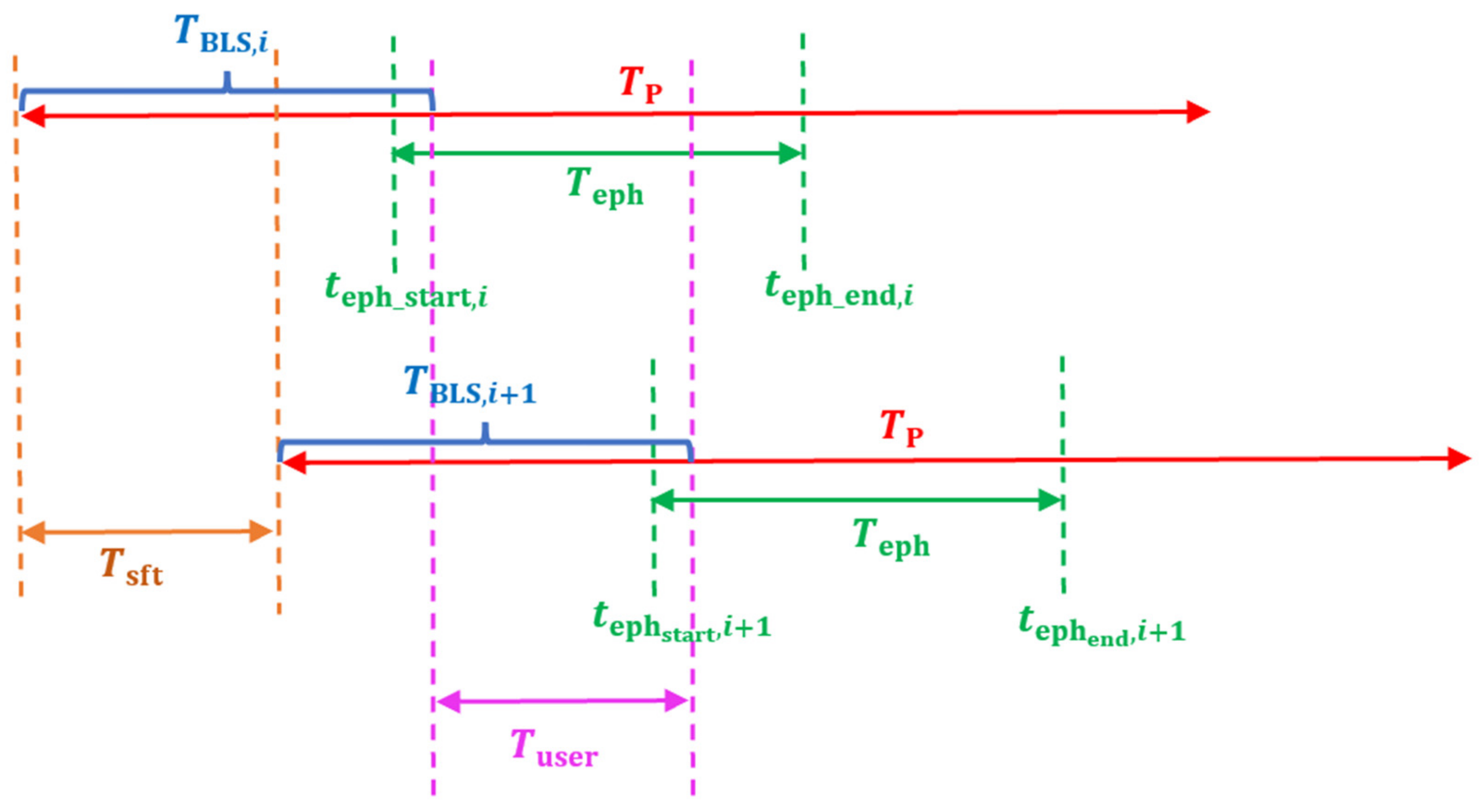
2.1. Near-Real-Time LEO Satellite POD with BLS Adjustment

Before the POD process, the GNSS measurements tracked by the GNSS receiver and antenna onboard the LEO satellite first needed to undergo data pre-processing screening, including outlier detection and cycle slip detection. Details were described in [24]. In this study, L1 and L2 phase and code GPS measurements were used to form the Ionosphere-Free (IF) combination for the BLS adjustment. Errors that could be computed well with models were corrected in the Observed-Minus-Computed (O-C) terms, including the LEO and GNSS satellite antenna Phase Center Offset (PCOs) and Phase Center Variations (PCVs), the corrections from the LEO satellite Antenna Phase Center (APC) to the Center of Mass (CoM), the phase windups, the relativistic effects and the Differential Code Biases (DCBs) (if needed) of the GNSS satellites, and the Sagnac effect.

The observation equations for the IF phase ($\Delta {\phi }_{\mathrm{IF}}^s$) and code O-C terms ($\Delta p_{\mathrm{IF}}^s$) for satellite $s$ at the $i$-th epoch $t_i$ could be expressed as follows:

$$\mathrm{E}\left(\Delta {\phi }_{\mathrm{IF}}^s\left(t_i\right)\right)=A_{\mathrm{K}}^s\left(t_i\right)X_{\mathrm{K}}+A_{\mathrm{SRP}}^s\left(t_i\right)a_{\mathrm{SRP}}+A_{\mathrm{Sto}}^s\left(t_i\right)a_{\mathrm{Sto}}+c\times \Delta t_r\left(t_i\right)+{\lambda }_{\mathrm{IF}}\times N_{\mathrm{IF}}^s$$

(1)

$$\mathrm{E}\left(\Delta p_{\mathrm{IF}}^s\left(t_i\right)\right)=A_{\mathrm{K}}^s\left(t_i\right)X_{\mathrm{K}}+A_{\mathrm{SRP}}^s\left(t_i\right)a_{\mathrm{SRP}}+A_{\mathrm{Sto}}^s\left(t_i\right)a_{\mathrm{Sto}}+c\times \Delta t_r\left(t_i\right)$$

(2)

where $\mathrm{E}\left(·\right)$ was the expectation operator. $\Delta t_r$ denoted the LEO satellite clock bias, which was multiplied with the speed of light $c$. ${\lambda }_{\mathrm{IF}}$ was the IF wavelength, which only had a mathematical meaning similar to the non-integer IF ambiguity $N_{\mathrm{IF}}^s$ of satellite $s$, where:

$${\lambda }_{\mathrm{IF}}=\frac{c}{f_1+f_2}$$

(3)

$$N_{\mathrm{IF}}^s=\frac{f_1^2{\lambda }_1{N}_1-f_2^2{\lambda }_2{N}_2}{c\left(f_1-f_2\right)}+\frac{{\xi }_{\mathrm{IF}}-{\xi }_{\mathrm{IF}}^s-d_{\mathrm{IF}}}{{\lambda }_{IF}}$$

(4)

$f_j$ and ${\lambda }_j$ denoted the frequency and wavelength of carrier $L_j$, respectively. ${\xi }_{\mathrm{IF}}$ and ${\xi }_{\mathrm{IF}}^s$ were the phase hardware biases of the LEO satellite and GNSS satellite $s$, respectively. $d_{\mathrm{IF}}$ denoted the code hardware bias of the LEO satellite, and the DCB of the GNSS satellites was assumed corrected in the O-C terms. New ambiguity parameter $N_{\mathrm{IF}}^s$ was set whenever a cycle slip occurs on L1 or L2.

In Equations (1) and (2), $X_{\mathrm{K}}$ denoted the six Keplerian elements of the LEO satellite orbit at the initial epoch $t_0$ of the BLS adjustment, i.e., the semi-major axis, the eccentricity, the inclination, the right ascension of ascending node, the argument of perigee, and the argument of latitude at $t_0$. $a_{\mathrm{SRP}}$ was a subset of $a_{\mathrm{SRP},\mathrm{all}}$, which contained nine elements, namely the constant, sine, and cosine terms of the Solar Radiation Pressure (SRP) accelerations in the radial (R), along-track (S), and cross-track (W) directions, expressed as:

$$a_{\mathrm{SRP},\mathrm{all}}={\left(a_{\mathrm{R}0},a_{\mathrm{S}0},a_{\mathrm{W}0},a_{\mathrm{RS}},a_{\mathrm{SS}},a_{\mathrm{WS}},a_{\mathrm{RC}},a_{\mathrm{SC}},a_{\mathrm{WC}}\right)}^{\mathrm{T}}$$

(5)

They formed the SRP accelerations in the radial ($a_{\mathrm{SRP},\mathrm{R}}$), along-track ($a_{\mathrm{SRP},\mathrm{S}}$), and cross-track ($a_{\mathrm{SRP},\mathrm{W}}$) directions as follows:

$$a_{\mathrm{SRP},\mathrm{R}}=a_{\mathrm{R}0}+a_{\mathrm{RS}}\times \sin \left(u\right)+a_{\mathrm{RC}}\times \cos \left(u\right)$$

(6)

$$a_{\mathrm{SRP},\mathrm{S}}=a_{\mathrm{S}0}+a_{\mathrm{SS}}\times \sin \left(u\right)+a_{\mathrm{SC}}\times \cos \left(u\right)$$

(7)

$$a_{\mathrm{SRP},\mathrm{W}}=a_{\mathrm{W}0}+a_{\mathrm{WS}}\times \sin \left(u\right)+a_{\mathrm{WC}}\times \cos \left(u\right)$$

(8)

where $u$ is the argument of latitude. To avoid overparameterization, $a_{\mathrm{SRP}}$ here contained only the constant terms $a_{\mathrm{R}0}$, $a_{\mathrm{S}0}$, and $a_{\mathrm{W}0}$. In Equations (1) and (2), $a_{\mathrm{Sto}}$ stood for the stochastic accelerations in the R, S, and W-directions, which were set for each sub-interval of 6 min. $a_{\mathrm{Sto}}$ was constrained to zero with a standard deviation of $5\times {10}^{-9} \mathrm{m}/{\mathrm{s}}^2$ to avoid over-parametrization. $A_{\mathrm{K}}^s$, $A_{\mathrm{SRP}}^s$, and $A_{\mathrm{Sto}}^s$ represented the partial derivatives of the IF phase and code observations from satellite $s$, with respect to the unknowns $X_{\mathrm{K}}$, $a_{\mathrm{SRP}}$, and $a_{\mathrm{Sto}}$, respectively. They could be formulated as:

$$A_{\mathrm{K}}^s\left(t_i\right)=\frac{X_{r0}\left(t_i\right)-X^s\left(t_i\right)}{\Vert X^s\left(t_i\right)-X_{r0}\left(t_i\right)\Vert }\times \frac{\partial X_{r0}\left(t_i\right)}{\partial X_{\mathrm{K}}}$$

(9)

$$A_{\mathrm{SRP}}^s\left(t_i\right)=\frac{X_{r0}\left(t_i\right)-X^s\left(t_i\right)}{\Vert X^s\left(t_i\right)-X_{r0}\left(t_i\right)\Vert }\times \frac{\partial X_{r0}\left(t_i\right)}{\partial a_{\mathrm{SRP}}}$$

(10)

$$A_{\mathrm{Sto}}^s\left(t_i\right)=\frac{X_{r0}\left(t_i\right)-X^s\left(t_i\right)}{\Vert X^s\left(t_i\right)-X_{r0}\left(t_i\right)\Vert }\times \frac{\partial X_{r0}\left(t_i\right)}{\partial a_{\mathrm{Sto}}}$$

(11)

where $X_{r0}\left(t_i\right)$ and $X^s\left(t_i\right)$ were the approximate LEO satellite position and the position of GNSS satellite $s$, respectively, at $t_i$. The term $\left(X_{r0}\left(t_i\right)-X^s\left(t_i\right)\right)/\Vert X^s\left(t_i\right)-X_{r0}\left(t_i\right)\Vert$ stood for the partial derivatives of the observations, with respect to the LEO satellite position at $t_i$. The partial derivatives of the LEO satellite position, with respect to the unknowns $X_{\mathrm{K}}$, $a_{\mathrm{SRP}}$, and $a_{\mathrm{Sto}}$ at $t_i$ were expressed as $\partial X_{r0}\left(t_i\right)/\partial X_{\mathrm{K}}$, $\partial X_{r0}\left(t_i\right)/\partial a_{\mathrm{SRP}}$, and $\partial X_{r0}\left(t_i\right)/\partial a_{\mathrm{Sto}}$, respectively. These terms are developed with numerical integration based on the variational equations [25].

Based on Equations (1) and (2), all the unknown parameters, i.e., $X_{\mathrm{K}}$, $a_{\mathrm{SRP}}$, $a_{\mathrm{Sto}}$, $\Delta t_r\left(t_i\right)$, and $N_{\mathrm{IF}}^s$ are estimated in the BLS adjustment. Real-time high-precision GNSS orbits and clocks were used for the adjustment. Equal weighting was applied here due to the simple measurement environment of the LEO satellite, which was also helpful in strengthening the model. The sampling interval and time span used for the processing can vary with the orbital accuracy needed. In this study, 24 h of data with a sampling interval of 30 s were used for our tests in Section 3.

With the estimated orbital dynamic parameters, denoted as ${\widehat{X}}_{\mathrm{K}}$, ${\widehat{a}}_{\mathrm{SRP}}$, and ${\widehat{a}}_{\mathrm{Sto}}$, the Cartesian coordinates of the LEO satellite orbit could be numerically integrated to any time point within the estimation time window, also with the help of the existing advanced models for Earth’s gravity and other perturbation accelerations. They are briefly described in

Table 1. Dynamic models used for orbit numerical integration.

Acceleration Terms	Models and Parameters Used
Gravitational Attraction of the Earth	EGM2008 (Earth Potential Degree: 120) [26]
Gravitational Attractions of other planets	Ephemeris from JPL DE405 [27]
Solid Earth and Pole Tides	IERS 2010 [28]
Ocean Tides	FES2004 [29]

.

With the real-time orbits calculated, the orbital errors could be analyzed with reference to the post-processed reference orbits generated with, e.g., the IGS final products. Compared to the orbital errors in the radial, along-track, and cross-track directions, the corresponding error projection on the Earth, i.e., the OURE, was more relevant for the ground user. In this study, the ${\sigma }_{\mathrm{OURE}}$ was calculated in a global averaged sense, based on the Root Mean Square (RMS) of the radial (${\sigma }_{\mathrm{R}}$), along-track (${\sigma }_{\mathrm{S}}$), and cross-track orbital errors (${\sigma }_{\mathrm{W}}$), as well as their projection coefficients (${\omega }_{\mathrm{R}}$, ${\omega }_{\mathrm{SW}}$) [1], expressed as:

$${\sigma }_{\mathrm{OURE}}=\sqrt{{\omega }_{\mathrm{R}}^2{\sigma }_{\mathrm{R}}^2+{\omega }_{\mathrm{SW}}^2\left({\sigma }_{\mathrm{S}}^2+{\sigma }_{\mathrm{W}}^2\right)}$$

(12)

To calculate the ${\sigma }_{\mathrm{OURE}}$ in a global averaged sense, the projection coefficients ${\omega }_{\mathrm{R}}$ and ${\omega }_{\mathrm{SW}}$ were computed based on integration in the longitude and latitude directions of the Earth [30]. ${\omega }_{\mathrm{R}}$ increases with the orbital height, while ${\omega }_{\mathrm{SW}}$ decreases with the orbital height. For GRACE C and Sentinel-3B tested in Section 3, ${\omega }_{\mathrm{R}}$ amounted to about 0.457 and 0.542, respectively, and ${\omega }_{\mathrm{SW}}$ amounted to about 0.629 and 0.594, respectively. By calculating the RMS in each direction, the outlier exclusion was optionally performed with a threshold comprising the mean error and 4.42 times the standard deviation. More details are given in Section 3.

2.2. Short-Term Orbit Prediction for Real-Time Applications

Using high-precision GNSS products, as stated in [18], the near-real-time orbits estimated with BLS adjustment in Section 2.1 could reach a 3D RMS below or around 5 cm. Next, the near-real-time LEO satellite orbits needed to be predicted in the near future so that the latency caused by the data collection, data processing, denoted as $T_{\mathrm{BLS}}$, and intervals between subsequent rounds of the BLS adjustments ($T_{\mathrm{Sft}}$) could be bridged. Assuming a fast and real-time data collection with ignorable latency, the prediction time $T_{\mathrm{P}}$ needed to be at least $T_{\mathrm{BLS}}+T_{\mathrm{Sft}}$, not to mention the possible occurrence of BLS processing problems, which may have required the users to use the previous round of the prediction. Assuming a processing time of 3–12 min and a time shift of 5 min between subsequent rounds of the BLS processing, a prediction time $T_{\mathrm{P}}$ of 30 min was considered in this section. Note that the real-time users only needed to use a part of the predicted orbits, depending on the $T_{\mathrm{BLS}}$ and $T_{\mathrm{Sft}}$.

Figure 2 shows the time scheme for the near-real-time BLS POD, the short-term orbit prediction, and the ephemeris fitting for the $i$-th and the ($i+1$)-th rounds of the processing. As an example, for the $i$-th round, the BLS POD endured a period of $T_{\mathrm{BLS},i}$ processing the data of, e.g., the last 24 h. The prediction started after the BLS POD, with the prediction period $(T_{\mathrm{P}}$) started by the end of the processed 24 h, i.e., at the beginning of the BLS processing (see the start of the top red line). The pre-defined prediction time, $T_{\mathrm{P}}$, was conservatively longer than it was actually needed. With the orbit prediction finished, the ephemeris fitting was performed using the predicted orbits at the regulated start and end time points $t_{\mathrm{eph}\_\mathrm{start},i}$ and $t_{\mathrm{eph}\_\mathrm{end},i}$, with a pre-defined fitting interval of $T_{\mathrm{eph}}$. Similar to the broadcast ephemeris of the GNSS satellites, $t_{\mathrm{eph}\_\mathrm{start},i}$ and $t_{\mathrm{eph}\_\mathrm{end},i}$ were often defined at integer times, where $t_{\mathrm{eph}\_\mathrm{start},i}$ could be considered slightly before the end of the BLS adjustment, although the real-time users did not use this part. Within the fitted ephemeris, the real-time users only use the part for which the last round of processing was completed, and the next round of processing was not yet finished (see the magenta line). From Figure 2, it could be observed that the period for real-time usage $T_{\mathrm{user}}$ equaled to the time shift between subsequent rounds of the BLS processing, $T_{\mathrm{Sft}}$. The processing time of the prediction and the ephemeris fitting were considered to be insignificant compared to the processing time of the BLS adjustment. Therefore, they were not further counted in Figure 2.

With the near-real-time high-accuracy BLS LEO satellite orbits available, a proper prediction strategy needs to be defined for a prediction time of up to 30 min. To achieve a possibly high orbital prediction accuracy, for a certain prediction period, the prediction strategy varies for LEO satellites at different altitudes. For Sentinel-3B at about 810 km altitude and GRACE C at about 500 km, as examples, the strategies for a 30 min orbital prediction were selected as strategy A, shown in

Table 2. Prediction strategies of the LEO satellites Sentinel-3B of about 810 km and GRACE C of about 500 km orbital heights above ground.

Satellite	Fitting Time (h)	Keplerian Elements	SRP	Stochastic Velocity Pulses
Sentinel-3B	4	Yes (6)	Yes (9)	None
GRACE C	12	Yes (6)	Yes (9)	Every 1 h

[21]. For Sentinel-3B, the satellite orbits are extended based on dynamic parameters fitted within the last four hours. The dynamic parameters include the six Keplerian elements ($X_{\mathrm{K}}$), and nine SRP parameters ($a_{\mathrm{SRP},\mathrm{all}}$). For GRACE C flying at lower altitude, in addition to these 12 dynamic parameters, the satellite orbits were extended with additional once-per-hour stochastic velocity pulses. The dynamic parameters were fitted within 12 h. The strategy was selected based on OURE at a half-hour prediction period for these two satellites in 2019 and 2020 [21].

Depending on the processing time of the BLS POD ($T_{\mathrm{BLS}}$) and the time shift between subsequent BLS POD processes ($T_{\mathrm{Sft}}$), as shown in Figure 2, a certain time window within the prediction period corresponded to the real-time window of the users ($T_{\mathrm{user}}$). With a possibly quick processing and a frequent shift of the BLS POD, this time window could be attempted to be very near the prediction start, so that small prediction errors could be guaranteed. In Section 3, with different computation efficiencies assumed, different time windows will be tested for these two satellites to estimate the approximate real-time orbital errors.

2.3. Ephemeris Fitting of the Predicted Orbits

Providing the users with Cartesian orbits at each epoch is not an efficient solution for real-time applications. For GNSS satellites, it is typical to transmit orbital corrections for the broadcast ephemeris received from the navigation message. The orbital corrections are typically constructed with low-order polynomials to extract the orbital corrections at the desired time instants. For LEO satellites, the situations are different. Due to the much lower altitudes of the LEO satellites, the fitting time of the ephemeris need to be significantly reduced to reach the same level of accuracy as the GNSS broadcast ephemeris [1]. Low-order polynomials could also hardly serve as corrections for high-precision orbits with a sampling interval similar to those for the GNSS satellites, as the LEO satellite orbits change much faster. As such, it is reasonable to directly describe the precise LEO satellite orbits with a set of ephemeris parameters fitted within a short time interval, e.g., 10–30 min. The fitting errors are generally dependent on the orbital heights, the fitting intervals, and the choices of the ephemeris parameters.

Different from the GNSS satellites, the LEO satellites are near-circular. This leads to an eccentricity of almost zero, and near-singularities at the argument of perigee $\omega$ and the mean anomaly $M$. These could result in a poor precision of the Keplerian elements when estimating them in their traditional forms. Studies have been performed with regard to the LEO-specific non-singularity parameters [31,32]. To avoid the near-singularities mentioned above, three of the traditional Keplerian elements, i.e., the eccentricity $e$, the argument of perigee $\omega$, and the mean anomaly $M$ are reformed as [32]:

$$e_x=e\times \cos \left(\omega \right)$$

(13)

$$e_y=e\times \sin \left(\omega \right)$$

(14)

$$\gamma =\omega +M$$

(15)

where $\gamma$ was a newly formed Keplerian element. ${\gamma }_0$ represented $\gamma$ at the reference epoch $t_e$. The six traditional Keplerian elements were thus turned into $e_x$, $e_y$, ${\gamma }_0$, the semi-major axis $a$, the inclination $I_0$, and the Right Ascension of Ascending Node (RAAN) ${\mathsf{\Omega }}_0$ (in addition to ${\omega }_{\mathrm{E}}\times \left(t-t_{\mathrm{G}0}\right)$). ${\omega }_{\mathrm{E}}$ was the Earth rotation rate, and $t_{\mathrm{G}0}$ denoted the beginning of the GPS week. Similar to the GPS ephemeris, nine other parameters were used to compensate for different periodic behaviors of the orbital parameters, which were the mean motion correction $\Delta n$, the inclination rate $\dot{I}$, the RAAN rate $\dot{\Omega }$, and the second-order harmonic coefficients $Cus2$, $Cuc2$, $Crs2$, $Crc2$, $Cis2$, $Cic2$. Together with the reference epoch $t_e$, they formed the 16 estimable ephemeris parameters for the LEO satellites (see

Table 3. Estimable ephemeris parameters for LEO satellites.

Number of Parameters	Estimable Ephemeris Parameters
	Basic	Additional
16	$t_e$$, e_x$$, e_y$$, {\gamma }_0$$, a$$, I_0$$, {\mathsf{\Omega }}_0$ $\Delta n$$, \dot{I}$$, \dot{\Omega }$ $Cus2$$, Cuc2$$, Crs2$$, Crc2$$, Cis2$$, Cic2$	--
18		$\dot{a}$$, \dot{n}$
20		$\dot{a}$$, \dot{n}$$, Crs3$$, Crc3$
22		$\dot{a}$$, \dot{n},$$Crs3$$, Crc3$$, Cis3$$, Cic3$

). Note that the estimable parameters $e_x$, $e_y$, ${\gamma }_0$ need to be transformed back into their traditional forms $e$, $\omega$, and $M_0$ before sending them to users:

$$e=\sqrt{e_x^2+e_y^2}$$

(16)

$$\omega =\arctan \left(\frac{e_y}{e_x}\right)$$

(17)

$$M_0={\gamma }_0-\omega$$

(18)

In addition to the 16 basic ephemeris parameters, more parameters can be used to further compensate for the rest of the harmonic behaviors and high-order rates of certain ephemeris parameters. In this study, examples are given in Table 3 to form the 18-, 20-, and 22-parameter ephemeris. Other combinations can also be made to form the 18-, 20-, and 22-parameters without introducing significant differences in the fitting errors [32]. The estimable ephemeris parameters were fitted using orbits of a certain interval with the least-squares adjustment. The partial derivations of the Cartesian orbits to the estimable parameters are described in [32,33].

As mentioned before, the ephemeris fitting errors are related to the orbital heights, the fitting interval, and the selected ephemeris parameters. So far, most studies have used post-processed high-precision LEO satellite orbits or simulated orbits to fit the ephemeris parameters. In Section 4, to check the feasibility of the ephemeris parameters for real-time applications, the ephemeris fitting errors of Sentinel-3B and GRACE C are discussed for predicted LEO satellite orbits that correspond to the real-time time windows, using 10 min fitting intervals and parameters of different numbers.

3. Test Results

In this section, the real-time LEO satellite orbits based on BLS POD and short-term prediction will be analyzed in three parts. Firstly, the near-real-time BLS POD solutions are discussed for their processing time, orbital accuracies, and OURE using data of the 810 km orbital height of Sentinel-3B and 500 km GRACE C, and the real-time GNSS satellite orbits and clocks from CNES and IGS RTS. Secondly, with different BLS processing times assumed, the predicted satellite orbits within different prediction time windows are discussed for their accuracies and OUREs. Thirdly, a part of the predicted orbits containing the real-time time window are fitted into ephemeris of different parameters. The fitting errors for these predicted orbits are discussed. The total error budget for the real-time LEO satellite orbits can then be presented under different situations. The reference orbits were taken from the Level 1B products of JPL for GRACE C [17], and from the European Space Operations Centre (ESOC) for Sentinel-3B.

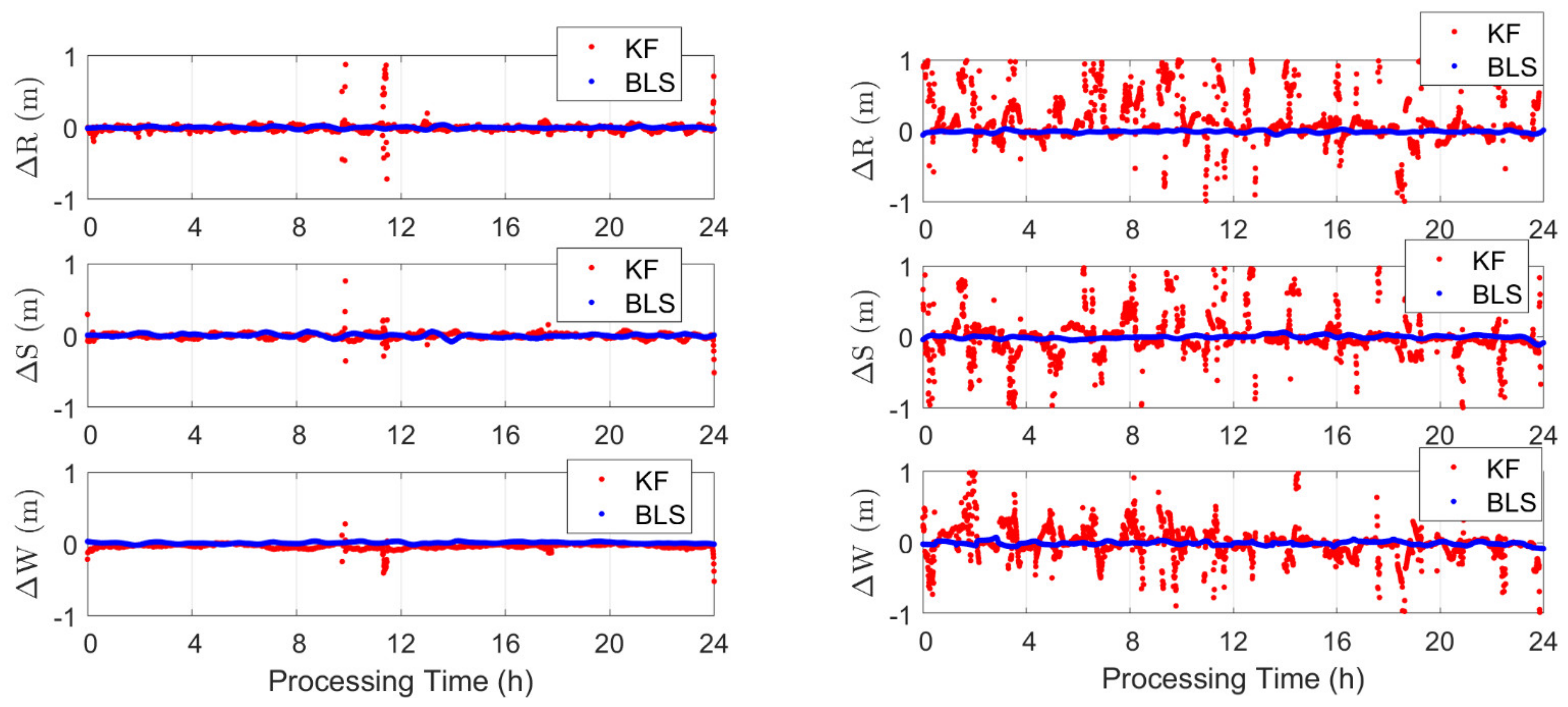
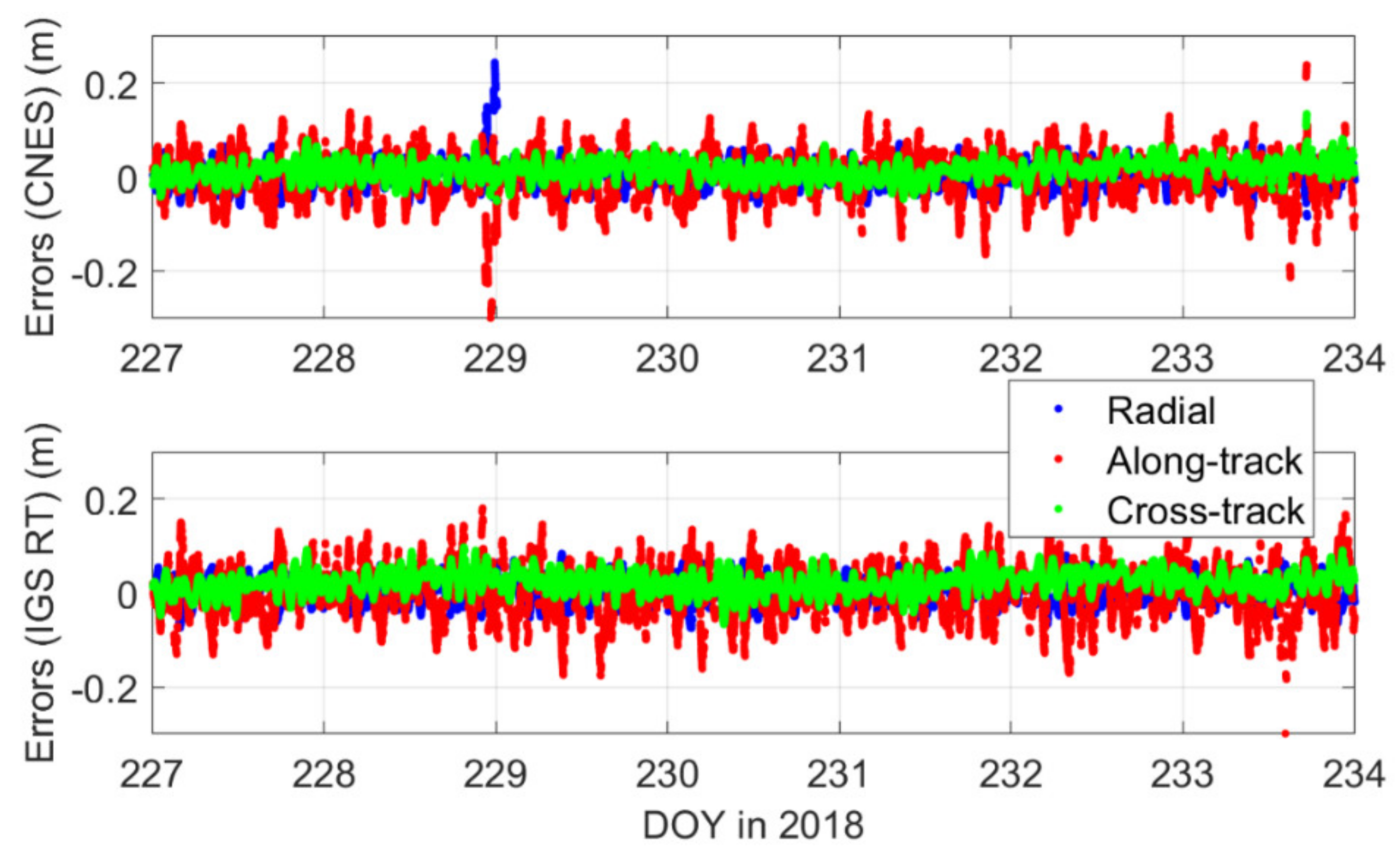
3.1. Near-Real-Time BLS POD Results

The accuracy of the near-real-time BLS POD results is closely related to that of the real-time GNSS products. Applying different GNSS products, the 3D RMS of the near-real-time BLS orbital errors could vary from a few centimeters to around 1 dm [18]. As representative examples, Figure 3 shows the BLS POD errors of Sentinel-3B on 15 August 2018 using the CNES real-time products and the IGS RTS products. Using 24 h of GPS L1 and L2 measurements with a sampling interval of 30 s, the RMS of the orbital errors in all three directions amounted to a few centimeters. The largest RMS can be found in the along-track direction due to the model deficiency as it cannot perfectly cover the air drag effects. The ${\sigma }_{\mathrm{OURE}}$, as calculated with Equation (12), amounted to 2.5 and 2.7 cm when using the two types of GNSS real-time products, respectively.

The good near-real-time BLS POD results shown in Figure 3 were not coincidences. With the starting time shifted by 5 min from 0:00:00 in GPS time (GPST) on 14 August 2018 to 23:55:00 on 20 August 2018, 2016, sets of 24 h daily BLS POD results were produced for Sentinel-3B. The corresponding daily RMS and ${\sigma }_{\mathrm{OURE}}$ are illustrated in Figure 4, with respect to their starting times. It could be seen that with a single-direction RMS amounting mostly from 1 to 4 cm, the ${\sigma }_{\mathrm{OURE}}$ using the CNES and IGS real-time products (see the gray dots) were generally between 2 and 4 cm. The along-track orbital errors were larger than those in the other two directions, which was caused by the air drag effects that were not perfectly compensated by the stochastic accelerations. The results obtained using the CNES real-time products (left panel) were slightly better than those generated using the IGS RTS products (right panel).

The averaged RMS, denoted as ${\overline{\sigma }}_{\mathrm{R}, \mathrm{S}, \mathrm{W}}$ in any of the R, S, W-directions, was calculated as follows:

$${\overline{\sigma }}_{\mathrm{R}, \mathrm{S}, \mathrm{W}}=\sqrt{\frac{{{\displaystyle \sum }}_{i-1}^n{\sigma }_{\mathrm{R},\mathrm{S},\mathrm{W}}^2\left(t_i\right)}{n}}$$

(19)

where ${\sigma }_{\mathrm{R}, \mathrm{S}, \mathrm{W}}$ represented the RMS of the orbital errors in any of the R, S, W-directions. $t_i$ denoted the starting time of the 24 h processing interval. $n$ denoted the number of the BLS processing rounds. The averaged ${\sigma }_{\mathrm{OURE}}$, denoted as ${\overline{\sigma }}_{\mathrm{OURE}}$, was similarly calculated as:

$${\overline{\sigma }}_{\mathrm{OURE}}=\sqrt{\frac{{{\displaystyle \sum }}_{i-1}^n{\sigma }_{\mathrm{OURE}}^2\left(t_i\right)}{n}}$$

(20)

Table 4. Averaged RMS of the orbital errors and the OUREs for Sentinel-3B and GRACE C using different real-time GNSS products. The results without outlier exclusions are given in parentheses.

Satellite	GNSS Real-Time Products	${\overline{\mathit{\sigma }}}_{\mathbf{R}} \left(\mathbf{cm}\right)$	${\overline{\mathit{\sigma }}}_{\mathbf{S}} \left(\mathbf{cm}\right)$	${\overline{\mathit{\sigma }}}_{\mathbf{W}} \left(\mathbf{cm}\right)$	${\overline{\mathit{\sigma }}}_{\mathbf{OURE}} \left(\mathbf{cm}\right)$	${\overline{\mathit{\sigma }}}_{3\mathbf{D}} \left(\mathbf{cm}\right)$
Sentinel-3B	CNES	1.6 (1.8)	2.9 (3.0)	2.3 (2.4)	2.4 (2.5)	4.1 (4.2)
	IGS RTS	1.8 (1.8)	3.4 (3.4)	3.1 (3.1)	2.9 (2.9)	4.9 (4.9)
GRACE C	CNES	1.2 (1.2)	2.2 (2.3)	1.9 (1.9)	1.9 (1.9)	3.2 (3.2)
	IGS RTS	1.4 (1.4)	2.6 (2.7)	2.0 (2.0)	2.1 (2.2)	3.5 (3.6)

lists the averaged RMS of the radial, along-track, and orbital errors, as well as the OUREs. The average 3D RMS was also given, which was calculated with the ${\overline{\sigma }}_{\mathrm{R}}$, ${\overline{\sigma }}_{\mathrm{S}}$, and ${\overline{\sigma }}_{\mathrm{W}}$. The RMS values without any outlier exclusion (see the end of Section 2.1) were also given in parentheses. From Table 4 it could be observed that the ${\overline{\sigma }}_{\mathrm{OURE}}$ of the near-real-time BLS POD were generally at 2–3 cm. The excluded outliers did not significantly influence the results. The averaged 3D RMSE were below 5 cm for the two test satellites using these two real-time GNSS products.

As shown in Figure 1, the status of the observation data was sometimes not optimal, which could result in frequent jumps, gaps, and outliers in the Kalman-filter-processed POD, even for well-maintained LEO satellites such as GRACE C. The day 12 August 2022 (see the right panel of Figure 1) was not coincidental. The Kalman-filter-based results, e.g., from 6 to 12 August 2022 exhibited similar behaviors as the red dots in the right panel of Figure 1. Using the BLS POD, the averaged RMS and OURE of the near-real-time orbits were processed for GRACE C in these seven days. The results (see

Table 5. Averaged RMS of the orbital errors and the OUREs for GRACE C in 6–12 August 2022 with less healthy data status. The results without outlier exclusions are given in parentheses.

Satellite	GNSS Real-Time Products	${\overline{\mathit{\sigma }}}_{\mathbf{R}} \left(\mathbf{cm}\right)$	${\overline{\mathit{\sigma }}}_{\mathbf{S}} \left(\mathbf{cm}\right)$	${\overline{\mathit{\sigma }}}_{\mathbf{W}} \left(\mathbf{cm}\right)$	${\overline{\mathit{\sigma }}}_{\mathbf{OURE}} \left(\mathbf{cm}\right)$	${\overline{\mathit{\sigma }}}_{3\mathbf{D}} \left(\mathbf{cm}\right)$
GRACE C	CNES	1.7 (1.7)	1.9 (2.0)	2.3 (2.3)	2.0 (2.0)	3.4 (3.5)
	IGS RTS	1.7 (1.7)	2.0 (2.0)	2.4 (2.4)	2.1 (2.1)	3.5 (3.5)

) suggested that this poor data status did not significantly influence the BLS POD accuracy. A similar OURE of about 2 cm could be achieved as in the test week of August 2018, using both the CNES and IGS real-time GNSS products.

In addition to the orbital accuracy, the processing time of the BLS POD process was of great concern, as it directly influenced the prediction time needed for real-time applications. Using 24 h of GPS L1 L2 observations with a sampling interval of 30 s, the processing time was tested on two servers of different settings (shown in

Table 6. Processing time of BLS POD on different servers.

Server Number	Model	Operating Frequency	Processing Time
1	Intel(R) Xeon(R)	2.7 GHz	5–6 min
2	Intel(R) Xeon(R)	1.9 GHz	11–12 min

). As shown in the table, with enough CPUs available, the operating frequency played an important role in the processing speed. The processing time increased from 5–6 min to 11–12 min with degraded computational operating frequency from 2.7 to 1.9 GHz. In Section 3.2, the variation of the processing time would be considered when testing different time windows for real-time usage of the predicted orbits.

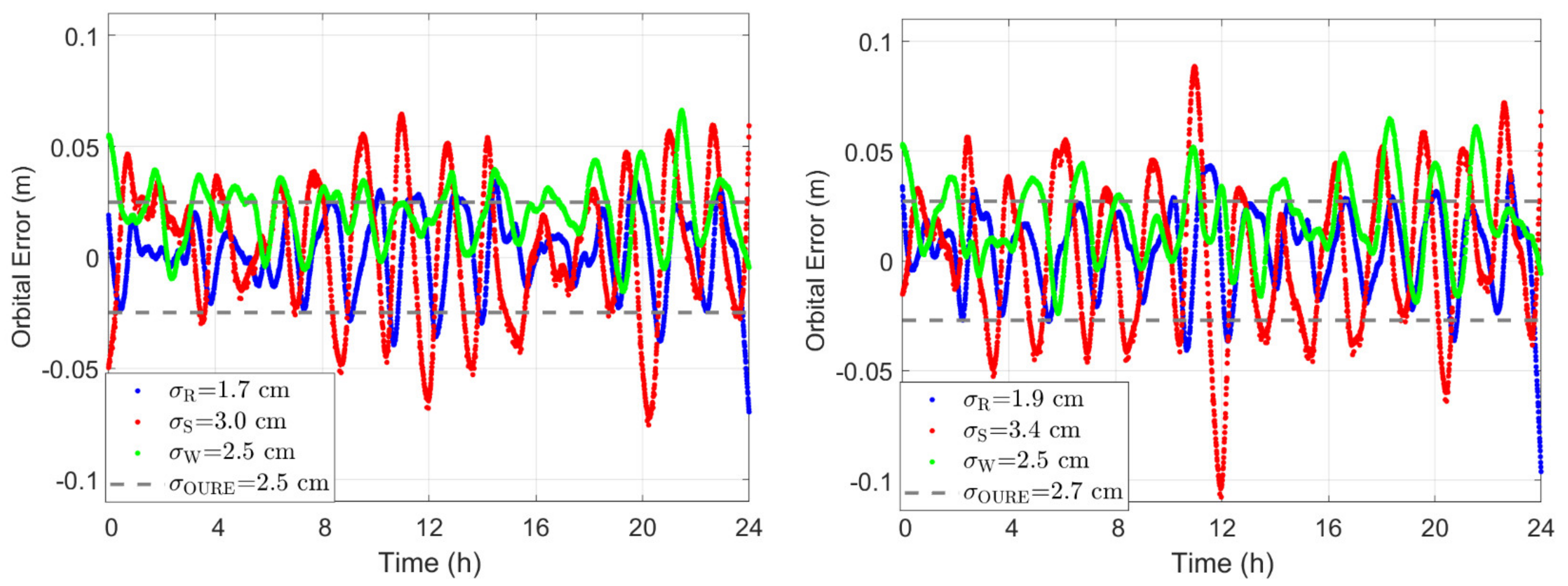
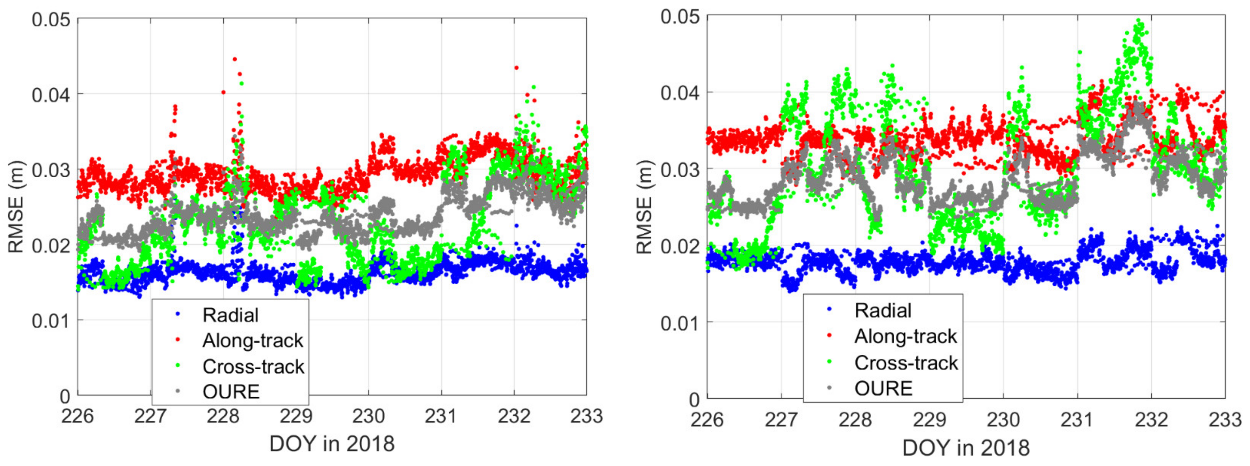
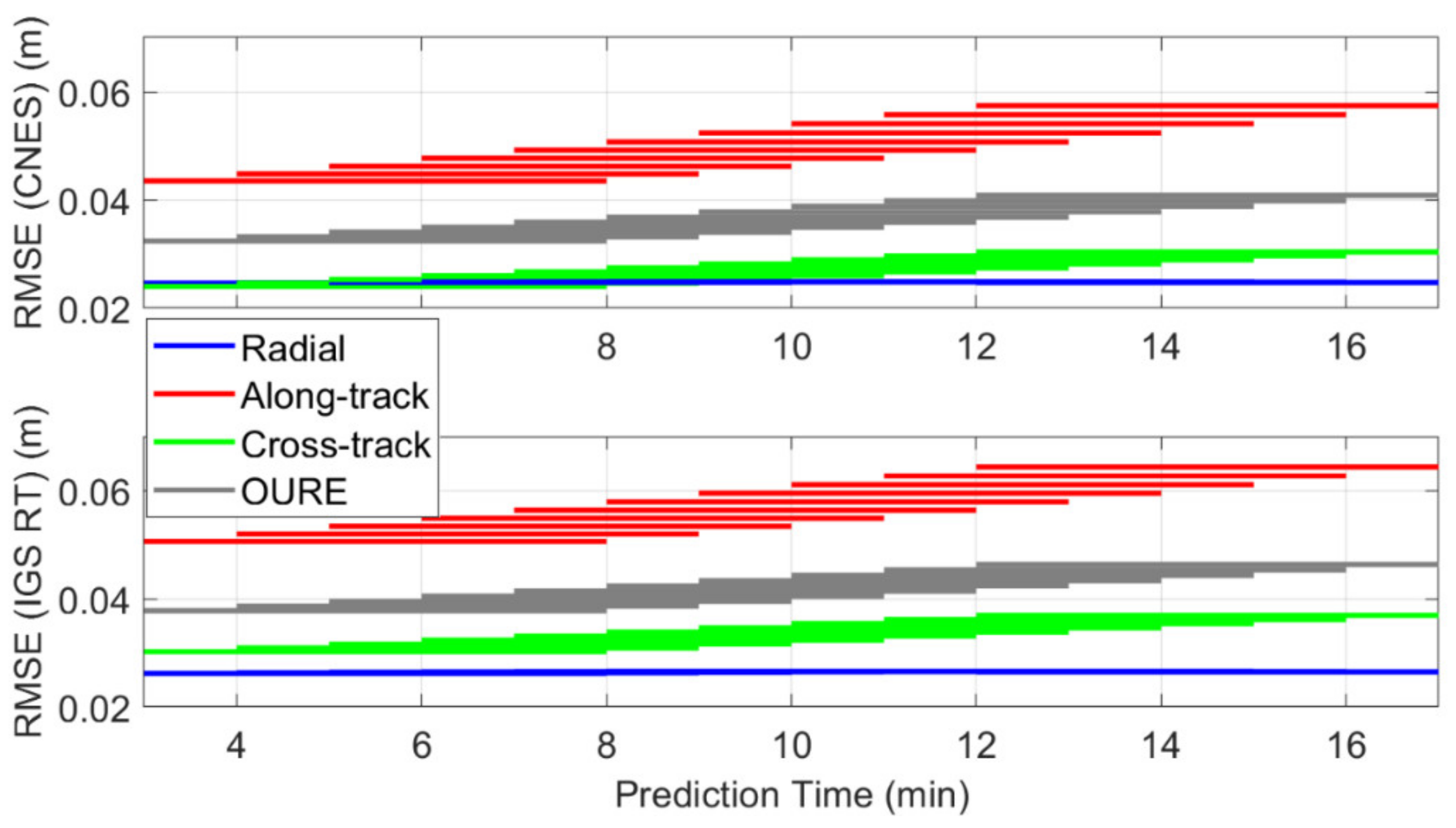
3.2. Real-Time Orbits Based on Short-Term Prediction

As described in Figure 2, the processing time of the BLS POD and the time shift between subsequent rounds of the BLS POD derived the needed prediction time, i.e., the time window that corresponded to the real-time usage in the predicted orbits. For a BLS processing time of $T_{\mathrm{BLS}}$ and a processing shift of $T_{\mathrm{Sft}}$, the real-time users would be able to use the predicted orbits at a prediction time from $T_{\mathrm{BLS}}$ to $T_{\mathrm{BLS}}+T_{\mathrm{Sft}}$. For a $T_{\mathrm{BLS}}$ of 5–6 min (see processor 1 in Table 6) and a $T_{\mathrm{Sft}}$ of 5 min, as an example, the orbits predicted from about 6–11 min would be used for real-time applications.

Figure 5 shows the predicted orbits of 6–11 min in each round of the 30 min predictions using the data of Sentinel-3B. The predicted orbits of the corresponding time windows were connected using different rounds of the predictions for assumed real-time applications from 15 to 21 August 2018. Using the CNES real-time products (see the top panel) as an example, the predicted orbital errors had an RMS of about 2.5, 4.8, and 2.6 cm in the radial, along-track, and cross-track directions, respectively, resulting in an OURE of 3.5 cm.

The RMS and OUREs for the predicted orbits at 6–11 min are listed in

Table 7. Averaged RMS of the predicted orbital errors at 6–11 min and the corresponding OUREs for Sentinel-3B and GRACE C using different real-time GNSS products. The results without outlier exclusions are given in parentheses.

Satellite	GNSS Real-Time Products	${\mathit{\sigma }}_{\mathbf{R},\mathbf{P}} \left(\mathbf{cm}\right)$	${\mathit{\sigma }}_{\mathbf{S},\mathbf{P}} \left(\mathbf{cm}\right)$	${\mathit{\sigma }}_{\mathbf{W},\mathbf{P}} \left(\mathbf{cm}\right)$	${\mathit{\sigma }}_{\mathbf{OURE},\mathbf{P}} \left(\mathbf{cm}\right)$	${\mathit{\sigma }}_{3\mathbf{D},\mathbf{P}} \left(\mathbf{cm}\right)$
Sentinel-3B	CNES	2.5 (2.6)	4.8 (5.4)	2.6 (2.6)	3.5 (3.8)	6.0 (6.5)
	IGS RTS	2.6 (2.6)	5.5 (5.5)	3.2 (3.2)	4.0 (4.1)	6.9 (6.9)
GRACE C	CNES	2.9 (3.2)	5.5 (6.3)	2.6 (2.6)	4.0 (4.5)	6.7 (7.8)
	IGS RTS	3.3 (3.5)	6.6 (7.0)	2.7 (2.7)	4.7 (5.0)	7.6 (8.2)

for Sentinel-3B and GRACE C using the CNES and IGS RTS products. ${\sigma }_{\mathrm{R},\mathrm{P}}$, ${\sigma }_{\mathrm{S},\mathrm{P}}$, ${\sigma }_{\mathrm{W},\mathrm{P}}$, and ${\sigma }_{3\mathrm{D},\mathrm{P}}$ denoted the RMS of the radial, along-track, cross-track, and 3D prediction errors at 6–11 min, respectively, and ${\sigma }_{\mathrm{OURE},\mathrm{P}}$ represented the corresponding OURE for the predicted orbits. From Table 7 it could be seen that the along-track prediction errors played the dominant role in the total error budget, especially for the lower LEO satellite GRACE C. Using high-quality real-time GNSS products, the OURE of the prediction errors at 6–11 min were generally at 3–5 cm. The 3D RMSE was at about 6–8 cm. Although the BLS near-real-time orbital accuracy of GRACE C was slightly better than that of Sentinel-3B (see Table 4), the short-term prediction accuracy of the lower satellite GRACE C was shown to be worse. For real-time LEO satellite orbital errors based on predictions of only 6–11 min, the orbital height already played an important role.

Depending on the BLS processing time ($T_{\mathrm{BLS}}$) on different machines, the valid prediction time windows used for real-time applications could vary. Assuming a processing time shift ($T_{\mathrm{Sft}}$) of 5 min, the prediction time windows were tested for 3–8 min, 4–9 min, 5–10 min, 6–11 min, 7–12 min, 8–13 min, 9–14 min, 10–15 min, 11–16 min, and 12–17 min. The RMS and OUREs of the predicted orbital errors are illustrated in Figure 6 for different prediction time windows. It could be seen that the prediction errors increased with the increasing prediction time, especially in the along-track direction (red lines). In the radial direction (blue lines), this increase was insignificant. For the Sentinel-3B at about 810 km, when using the CNES real-time products, the OURE (gray lines) had increased from 3.2 cm (using the prediction time window of 3–8 min) to 4.0 cm (using the prediction time window of 12–17 min). When using the IGS RTS products, the OURE had increased from 3.8 to 4.5 cm. The quality of the real-time GNSS products used, i.e., the accuracy of the near-real-time BLS orbits, also played a significant role in the orbital prediction.

The OUREs for the two test satellites using the CNES and IGS real-time products are listed in

Table 8. Averaged OURE of the predicted orbits within different prediction time windows. The results without outlier exclusions are given in parentheses.

Prediction Time Window (min)	Sentinel-3B (CNES) (cm)	Sentinel-3B (IGS RTS) (cm)	GRACE C (CNES) (cm)	GRACE C (IGS RTS) (cm)
3–8	3.2 (3.6)	3.8 (3.8)	3.6 (4.0)	4.2 (4.4)
4–9	3.3 (3.7)	3.9 (3.9)	3.7 (4.2)	4.4 (4.6)
5–10	3.4 (3.7)	4.0 (4.0)	3.9 (4.4)	4.5 (4.8)
6–11	3.5 (3.8)	4.0 (4.1)	4.0 (4.5)	4.7 (5.0)
7–12	3.6 (3.9)	4.1 (4.2)	4.2 (4.7)	5.0 (5.1)
8–13	3.7 (4.0)	4.2 (4.3)	4.4 (4.9)	5.1 (5.3)
9–14	3.8 (4.1)	4.3 (4.4)	4.5 (5.1)	5.3 (5.5)
10–15	3.9 (4.2)	4.4 (4.5)	4.7 (5.3)	5.4 (5.7)
11–16	4.0 (4.2)	4.5 (4.5)	4.9 (5.4)	5.6 (5.9)
12–17	4.1 (4.3)	4.6 (4.7)	5.0 (5.6)	5.8 (6.1)

for different prediction time windows. For the tested prediction windows from 3–8 min to 12–17 min, the OURE generally varied between 3 and 6 cm. From Table 8, it could be concluded that the real-time LEO satellite orbital accuracy based on BLS near-real-time POD and short-term predictions was mainly determined by the following factors:

1)

The prediction time, i.e., the sum of the BLS POD processing time ($T_{\mathrm{BLS}}$) and the time shift between subsequent BLS POD processes ($T_{\mathrm{Sft}}$). Extending the prediction time by 9 min, as shown in Table 8, had increased the averaged OURE by 0.8 to 1.6 cm. The increase was especially large for satellites with low altitudes.

2)

The orbital height. This factor has correlated influences with the prediction time on the real-time orbital accuracy. According to Table 8, compared to the 810 km Sentinel-3B, the GRACE C at 500 km had increased the OURE by about 4 mm at a short prediction window of 3–8 min, and by about 0.9–1.2 cm at a longer prediction window of 12 to 17 min.

3)

The quality of the GNSS satellite and clock products, i.e., the near-real-time BLS POD accuracy. By using CNES and IGS high-precision real-time GNSS products, the OURE had varied by 5–8 mm. The variation could increase when using other real-time GNSS products with lower accuracies.

In addition to the factors mentioned above, an appropriate prediction strategy is important for achieving good short-term prediction accuracy. A non-optimal prediction strategy, as tested, could easily lead to degradations of accuracy at some centimeters. The prediction strategies used in this contribution (see Table 2) were selected based on studies using high-precision post-processed orbits of these two satellites [21]. For other satellites, it is suggested to test for different prediction strategies using enough empirical data of a relevant period.

Similar to the last sub-section, the GRACE C data in 6–12 August 2022 with a low optimal data status was tested for short-term orbit prediction. It should be noted that from 2018 to 2022, the orbital height of GRACE C had reduced from about 503.3 km to 500.7 km. As shown in

Table 9. Averaged OURE of the predicted orbits of GRACE C with less healthy data and reduced height from 6 to 12 August 2022. The results without outlier exclusions are given in parentheses.

Prediction Time Window (min)	GRACE C (CNES) (cm)	GRACE C (IGS RTS) (cm)
3–8	4.9 (5.1)	4.9 (5.1)
4–9	5.2 (5.4)	5.2 (5.4)
5–10	5.4 (5.6)	5.5 (5.6)
6–11	5.7 (5.9)	5.7 (5.9)
7–12	6.0 (6.2)	6.0 (6.2)
8–13	6.3 (6.5)	6.3 (6.5)
9–14	6.6 (6.8)	6.6 (6.8)
10–15	6.9 (7.1)	7.0 (7.1)
11–16	7.2 (7.4)	7.3 (7.4)
12–17	7.5 (7.7)	7.7 (7.8)

, the prediction OURE had increased by about 1–3 cm for GRACE C in 2022. The degradation was possibly related to the following reasons:

1)

The already low orbital altitude had been further reduced in 2022. This led to increased influences of the mis-modeled air drag effects, which led to increased prediction errors.

2)

As data sets in different years were used, the data status and the variation of the stochastic accelerations were also changed. These might lead to slight differences in the predictions.

However, with advanced processing units having prediction time windows of 6–11 min or lower, it could be seen that the prediction OURE was generally at the sub-dm level. The reasons above that led to possible degradations of the prediction results mainly influence the orbit in relatively longer prediction windows.

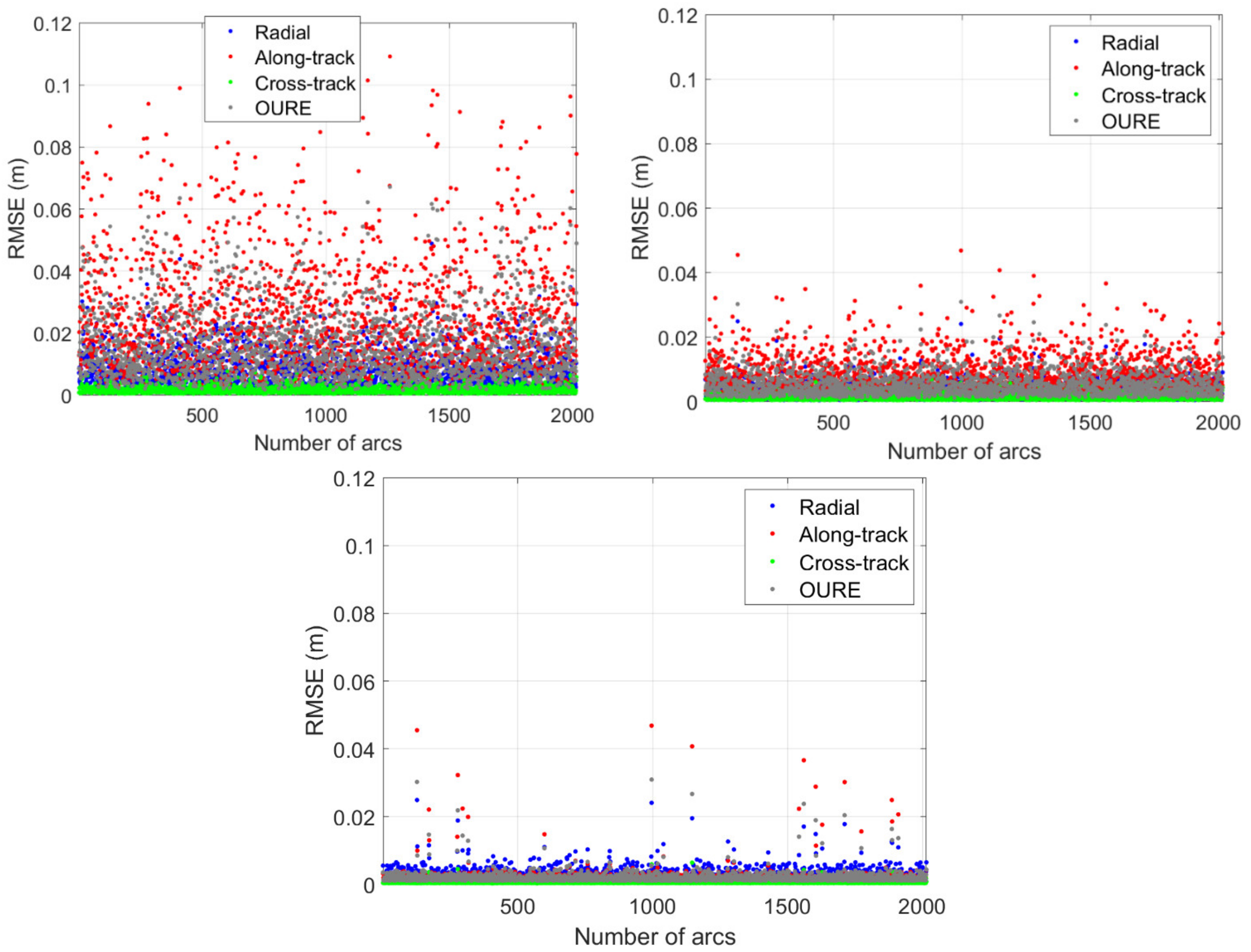
3.3. Ephemeris Fitting of the Real-Time Orbits

As the orbital information of LEO satellites varies quickly with time, instead of transmitting high-sampling orbits/orbit corrections, the LEO satellite orbits over short intervals could be represented by LEO-specific ephemeris parameters as described in Section 2.3. The orbital fitting errors are closely related to the following factors [32]:

1)

The orbital height

2)

The number of the ephemeris parameters

3)

The fitting interval

In general, a high altitude of the LEO satellite, a high number of the ephemeris parameters, and a short fitting interval are helpful in reducing the fitting errors. In this section, a fitting time of 10 min, i.e., from 5 to 15 min in the predicted orbits, was used to cover most of the 5 min prediction time windows described in the last sub-section. Different from fitting the post-processed high-precision orbits, as performed in most of the previous studies, this section used the predicted orbits for ephemeris fitting, which matched better to the actual real-time scenario. The data of 810 km height Sentinel-3B orbits and 500 km GRACE C orbits from 15 to 21 August 2018 were used for the tests.

Using Sentinel-3B data and the CNES real-time products as an example, Figure 7 shows the RMS of the ephemeris fitting errors for 2014 sets of 10 min fitting intervals, using the 5–15 min predicted orbits with the prediction start shifted by 5 min each time. The three sub-figures illustrated the cases for 16-, 18-, and 22-parameter fitting, respectively (see Section 2.3). The averaged RMSE of the ephemeris fitting errors and the averaged OURE are calculated as in Equations (19) and (20). For the Sentinel-3B orbits, the averaged OURE amounts to 1.9, 0.6, and 0.3 cm for the 16-, 18-, and 22-parameter fitting, respectively. Among the three directions, the along-track fitting errors played a major in the error budget.

The averaged RMSE and OURE of the fitting errors are listed in

Table 10. Averaged RMS and OURE of the ephemeris fitting errors for the predicted orbits of 5–15 min. The results without outlier exclusions are given in parentheses.

RMSE/OURE	Sentinel-3B (CNES) (cm)	Sentinel-3B (IGS RTS) (cm)	GRACE C (CNES) (cm)	GRACE C (IGS RTS) (cm)
16 Parameters
Radial	1.0 (1.0)	1.0 (1.0)	2.2 (2.2)	2.2 (2.2)
Along-track	3.0 (3.0)	3.0 (3.0)	5.2 (5.2)	5.2 (5.2)
Cross-track	0.2 (0.2)	0.2 (0.2)	0.5 (0.5)	0.5 (0.5)
OURE	1.9 (1.9)	1.9 (1.9)	3.4 (3.4)	3.4 (3.4)
18 Parameters
Radial	0.4 (0.4)	0.4 (0.4)	1.0 (1.0)	1.0 (1.0)
Along-track	1.0 (1.0)	1.0 (1.0)	2.1 (2.1)	2.1 (2.1)
Cross-track	0.2 (0.2)	0.2 (0.2)	0.5 (0.5)	0.5 (0.5)
OURE	0.6 (0.6)	0.6 (0.6)	1.4 (1.4)	1.4 (1.4)
22 Parameters
Radial	0.3 (0.3)	0.3 (0.3)	0.9 (0.9)	0.9 (0.9)
Along-track	0.4 (0.4)	0.4 (0.4)	1.2 (1.2)	1.2 (1.2)
Cross-track	0.1 (0.1)	0.1 (0.1)	0.2 (0.2)	0.2 (0.2)
OURE	0.3 (0.3)	0.3 (0.3)	0.9 (0.9)	0.9 (0.9)

for different situations. It could be seen that with a fitting interval of 10 min, the OURE of the fitting errors for Sentinel-3B were at a few millimeters for 18 and 22-parameter fitting, while the OURE was at 1–2 cm when using 16 ephemeris parameters. The differences in fitting errors could also be caused by the orbital height of the LEO satellite. For the much lower satellite GRACE C, the fitting errors were shown to be larger, i.e., with an OURE at 3–4 cm for the 16-parameter fitting, and slightly below 1 cm for the 22-parameter fitting. Different real-time GNSS products do not lead to significant differences in the ephemeris fitting errors. Compared with the prediction errors shown in Section 3.2, the fitting errors were generally insignificant when using 18 or more ephemeris parameters.

With the data in 6–12 August 2022 tested as before, the fitting errors of GRACE C were almost the same as those exhibited in Table 10. This suggested that the fitting errors were not influenced much by the sizes of the prediction errors when using the same dynamic models to extend the orbits. The orbital height and the model used to extend the orbits played a larger role in the fitting error budget.

3.4. Total Error Budget

Based on the short-term orbit prediction and the ephemeris fitting introduced in Section 3.2 and Section 3.3, the total error budget is discussed in this section. The real-time orbital errors on the user side corresponded to the differences between the Cartesian coordinates generated with the ephemeris parameters and the reference orbits. Assuming a BLS processing time ($T_{\mathrm{BLS}}$) varying from 5 to 10 min and a processing shift ($T_{\mathrm{Sft}}$) of 5 min, the time window corresponding to the real-time usage was tested for a prediction time of 5–10 min, 6–11 min, 7–12 min, 8–13 min, 9–14 min, and 10–15 min. The ephemeris fitting was performed using the 5–15 min predicted orbits, i.e., with a fitting interval of 10 min.

Table 11. Total error budget (in OURE) of the real-time LEO satellite orbits. The values are given for different prediction time windows. The results without outlier exclusions are given in parentheses.

Error Type	OURE (cm)
	5–10 min	6–11 min	7–12 min	8–13 min	9–14 min	10–15 min
Sentinel-3B (CNES)
Prediction error	3.4 (3.7)	3.5 (3.8)	3.6 (3.9)	3.7 (4.0)	3.8 (4.1)	3.9 (4.2)
Fitting error	0.2 (0.3)	0.2 (0.3)	0.2 (0.3)	0.2 (0.3)	0.2 (0.3)	0.2 (0.3)
Total error	3.4 (3.8)	3.5 (3.9)	3.6 (3.9)	3.7 (4.0)	3.8 (4.1)	3.9 (4.2)
Sentinel-3B (IGS RTS)
Prediction error	4.0 (4.0)	4.0 (4.1)	4.1 (4.2)	4.2 (4.3)	4.3 (4.4)	4.4 (4.5)
Fitting error	0.2 (0.3)	0.2 (0.3)	0.2 (0.3)	0.2 (0.3)	0.2 (0.3)	0.2 (0.3)
Total error	4.0 (4.0)	4.1 (4.1)	4.1 (4.2)	4.2 (4.3)	4.3 (4.4)	4.4 (4.5)
GRACE C (CNES)
Prediction error	3.9 (4.4)	4.0 (4.5)	4.2 (4.7)	4.4 (4.9)	4.5 (5.1)	4.7 (5.3)
Fitting error	0.6 (0.9)	0.6 (0.8)	0.6 (0.8)	0.6 (0.8)	0.6 (0.8)	0.6 (0.9)
Total error	4.0 (4.4)	4.1 (4.6)	4.3 (4.8)	4.4 (5.0)	4.6 (5.1)	4.8 (5.3)
GRACE C (IGS RTS)
Prediction error	4.5 (4.8)	4.7 (5.0)	5.0 (5.1)	5.1 (5.3)	5.3 (5.5)	5.4 (5.7)
Fitting error	0.6 (0.9)	0.6 (0.8)	0.6 (0.8)	0.6 (0.9)	0.6 (0.8)	0.6 (0.9)
Total error	4.6 (4.8)	4.8 (5.0)	5.0 (5.2)	5.1 (5.4)	5.3 (5.6)	5.5 (5.8)

shows the total error budget of the real-time orbits in OURE. The orbits were fitted using 22 ephemeris parameters, and only the fitting errors within the corresponding 5 min prediction time windows were counted for calculating their OUREs. From Table 11 it could be observed that the prediction errors played a major role in the total error budget, while the fitting errors had almost no influence on the total orbital errors. The orbital heights significantly affected the total errors. For Sentinel-3B at around 810 km height, the total real-time orbital errors were around 3–4 cm. For LEO satellites with higher orbits, the results were expected to be not worse than this level.

The total error budget was also given for GRACE C from 6–12 August 2022 with a lower healthy data status than above (

Table 12. Total error budget (in OURE) of the real-time GRACE C satellite orbits from 6 to 12 August 2022 with less healthy data status. The values are given for different prediction time windows. The results without outlier exclusions are given in parentheses.

Error Type	OURE (cm)
	5–10 min	6–11 min	7–12 min	8–13 min	9–14 min	10–15 min
GRACE C (CNES) in August 2022
Prediction error	5.4 (5.6)	5.7 (5.9)	6.0 (6.2)	6.3 (6.5)	6.6 (6.8)	6.9 (7.1)
Fitting error	0.6 (0.9)	0.6 (0.9)	0.6 (0.9)	0.6 (0.9)	0.6 (0.9)	0.6 (0.9)
Total error	5.5 (5.7)	5.8 (5.9)	6.0 (6.2)	6.3 (6.5)	6.6 (6.8)	6.9 (7.1)
GRACE C (IGS RTS) in August 2022
Prediction error	5.5 (5.6)	5.7 (5.9)	6.0 (6.2)	6.3 (6.5)	6.6 (6.8)	7.0 (7.1)
Fitting error	0.6 (0.9)	0.6 (0.9)	0.6 (0.9)	0.6 (0.9)	0.6 (0.9)	0.6 (0.9)
Total error	5.5 (5.7)	5.8 (5.9)	6.0 (6.2)	6.3 (6.5)	6.6 (6.8)	6.9 (7.1)

). Similarly, the prediction errors played the determining role in the total error budget. The real-time orbital errors were around 5–7 cm for different time windows.

Despite the various advantages of the BLS adjustment, the real-time LEO satellite orbital accuracy based on BLS POD and short-term prediction was shown to be no worse than the sub-dm-level LEO satellite POD based on the real-time Kalman filter, especially for satellites with relatively high altitudes. As such, for high-altitude LEO satellites with orbits higher than 800 km, the proposed strategy based on BLS POD and short-term prediction was a reasonable method for applications requiring high-accuracy and real-time orbits.

4. Discussions and Conclusions

Benefiting from the much lower altitudes of the LEO satellites and their correspondingly increased speeds, LEO augmentation is nowadays frequently discussed in aiding the traditional GNSS-based PNT service. Similar to the GNSS satellites, for ground-based real-time PNT service, the orbits and clocks of the LEO satellites need to be provided to users in real time with high precision. Among them, high-precision and stable real-time orbits are of the utmost importance, as the real-time satellite clocks often need to be determined by constraining or fixing the predicted orbits.

Compared to the real-time orbits determined with the Kalman filter, the Batch Least-Squares (BLS) POD process is often less vulnerable to data problems, as the nature of the BLS allows the usage of information from both sides and at the same time, guarantees a better data pre-processing results. However, BLS usually suffers from longer processing time, and is thus less efficient than Kalman-filter-based processing in real time applications. With the ever-improving computational power nowadays and the advanced orbit prediction strategies, it is possible to limit the prediction time and the short-term orbital prediction errors. In this study, a comprehensive analysis is performed with regard to the procedure and the accuracy of the real-time LEO orbits based on BLS adjustment and short-term prediction. The process starts from the raw GNSS observations tracked onboard the LEO satellites, and ends with the LEO-specific ephemeris parameters that are broadcast to users in real time.

Using real LEO satellite data of two satellites at different altitudes, i.e., the GRACE C at about 500 km and Sentinel-3B at about 810 km, the study is split into three parts addressing different points, i.e., the near-real-time BLS POD, the short-term predictions, and the ephemeris fitting. A variation of reasonable BLS processing times is assumed to test the shifted prediction windows that will be needed for real-time applications. Two types of high-precision real-time GNSS products, i.e., the CNES real-time products and the IGS RTS products, are used to test their influences on the BLS POD results and the corresponding short-term prediction. Using 24 h dual-frequency GPS data with a sampling interval of 30 s, high-accuracy near-real-time orbits with an OURE of about 1–3 cm can be obtained using the BLS adjustment, for both satellites and using both products.

For the real-time orbital errors achieved in the total error budget, the following points are to be noted:

1)

Shortening the BLS processing time is essential, as it directly relates to the valid prediction time to be used in the real-time window. In our tests, for the same satellite, extending the BLS processing time from 3 to 12 min could increase the prediction OURE by 0.8 to 1.6 cm. Within this range, a larger increase is often observed for the lower LEO satellite GRACE C.

2)

The orbital height plays an important role in the orbit prediction and ephemeris fitting, especially when the number of ephemeris parameters is low. Comparing the results of the 810 km height Sentinel-3B and the 500 km GRAEC C, for a long BLS processing time of 12 min, the increase in the OURE for the orbit prediction amounts to about 1 cm. For 16-parameter ephemeris fitting, the OURE of the fitting error itself has reached 1.5 cm.

3)

Assuming ephemeris fitting with, e.g., 22 parameters and a short fitting interval of 10 min, the real-time orbital errors are dominated by the errors in the predicted orbits, where the along-track errors have the major contribution. In general, with a current modern processing unit limiting the BLS processing time to 5–6 min, a real-time OURE of 3–5 cm can be achieved when an appropriate prediction strategy is applied and when high-quality GNSS products are used.

4)

It is suggested to study the best suitable prediction strategy for a specific LEO satellite within a specific time period, especially for low-altitude satellites. Otherwise, the prediction errors could increase.

5)

In this study, two types of high-quality real-time GNSS products were used in the BLS POD process, i.e., the CNES real-time products and the IGS RTS products. The resulting differences in the POD showed that the CNES real-time GNSS products had delivered near-real-time orbits with better accuracy. However, the purpose of using these two different real-time GNSS products here is not to compare them, but to show that the GNSS orbits and clocks influence the LEO POD results, even when both products are of high accuracy. When GNSS products are only available at a lower accuracy, e.g., the predicted part of the IGS ultra-rapid products, the POD accuracy will correspondingly decrease.

6)

This contribution addressed only the orbital contribution to the URE. For ground-based positioning users, the combined contribution of the orbital and clock errors is of actual concern. Although not further attempted in this paper, the method to determine real-time LEO satellite clocks, their accuracies, and their correlations with real-time orbits are topics that will be considered in our future work.

Despite all the advantages of the BLS adjustment and the high accuracy that can be achieved in actual real time, one has to admit that the Kalman filter is more flexible in dealing with orbits that are difficult to be modeled and predicted, e.g., orbits during maneuvers, and very low LEO satellite orbits below, e.g., 300 km. This flexibility originates from its much shorter processing time of one epoch, which leads to very short prediction. For the BLS POD, shortening the processing time is one of the essential tasks in the future, especially for LEO satellites with low altitudes. This concerns not only the expectation of faster processing units in the future, but also the capability to compromise between the accuracy of the near-real-time orbits, and the amount of the observation data used. In general, BLS POD with short-term orbit prediction is shown to be a promising method for obtaining high-accuracy real-time LEO satellite orbits, especially for high-altitude LEO satellites. Further improvements can be expected in the future with improvements in computational efficiency.

References

1. Reid, T.G.R.; Neish, A.M.; Walter, T.; Enge, P.K. Broadband LEO constellations for navigation. Navig. J. Inst. Navig. 2018, 65, 205–220. [Google Scholar] [CrossRef]
2. Baeza, V.M.; Lagunas, E.; Al-Hraishawi, H.; Chatzinotas, S. An Overview of Channel Models for NGSO Satellites. In Proceedings of the IEEE Vehicular Technology Conference 2022, London, UK, Beijing, China, 26–29 September 2022. [Google Scholar] [CrossRef]
3. Montenbruck, O.; Gill, E. Around the world in a hundred minutes. In Satellite Orbits, 1st ed.; Springer: Berlin, Germany, 2000; pp. 1–13. [Google Scholar]
4. Ge, H.; Li, B.; Ge, M.; Zang, N.; Nie, L.; Shen, Y.; Schuh, H. Initial assessment of precise point positioning with LEO enhanced global navigation satellite systems (LeGNSS). Remote Sens. 2018, 10, 984. [Google Scholar] [CrossRef] [Green Version]
5. Li, X.; Ma, F.; Li, X.; Lv, H.; Bian, L.; Jiang, Z.; Zhang, X. LEO constellation-augmented multi-GNSS for rapid PPP convergence. J. Geod. 2018, 93, 749–764. [Google Scholar] [CrossRef]
6. Li, M.; Xu, T.; Guan, M.; Gao, F.; Jiang, N. LEO-constellation-augmented multi-GNSS real-time PPP for rapid re-convergence in harsh environments. GPS Solut. 2022, 26, 29. [Google Scholar] [CrossRef]
7. Wang, K.; El-Mowafy, A.; Wang, W.; Yang, L.; Yang, X. Integrity Monitoring of PPP-RTK Positioning; Part II: LEO Augmentation. Remote Sens. 2022, 14, 1599. [Google Scholar] [CrossRef]
8. Faragher, R.; Ziebart, M. OneWeb LEO PNT: Progress or Risky Gamble? Inside GNSS, 28 September 2020. Available online: https://insidegnss.com/oneweb-leo-pnt-progress-or-risky-gamble/ (accessed on 28 June 2021).
9. Lawrence, D.; Cobb, H.S.; Gutt, G.; O’Connor, M.; Reid, T.G.R.; Walter, T.; Whelan, D. Innovation: Navigation from LEO. GPS World, 30 June 2017. Available online: https://www.gpsworld.com/innovation-navigation-from-leo/ (accessed on 10 October 2022).
10. Jia, Y.; Bian, L.; Cao, Y.; Meng, Y.; Zhang, L. Design and Analysis of Beidou Global Integrity System Based on LEO Augmentation. In Lecture Notes in Electrical Engineering, Proceedings of the China Satellite Navigation Conference (CSNC) 2020 Proceedings: Volume II, CSNC 2020, Chengdu, China, 22–25 November 2020; Sun, J., Yang, C., Xie, J., Eds.; Springer: Singapore, 2020; Volume 651, pp. 624–633. [Google Scholar] [CrossRef]
11. Michalak, G.; Glaser, S.; Neumayer, K.H.; König, R. Precise orbit and Earth parameter determination supported by LEO satellites, inter-satellite links and synchronized clocks of a future GNSS. Adv. Space Res. 2021, 12, 4753–4782. [Google Scholar] [CrossRef]
12. Yang, L. The Centispace-1: A LEO Satellite-Based Augmentation System. In Proceedings of the 14th Meeting of the International Committee on Global Navigation Satellite Systems, Bengaluru, India, 8–13 December 2019. [Google Scholar]
13. Hauschild, A.; Tegedor, J.; Montenbruck, O.; Visser, H.; Markgraf, M. Precise onboard orbit determination for LEO satellites with real-time orbit and clock corrections. In Proceedings of the ION GNSS+ 2016, Institute of Navigation, Portland, OR, USA, 12–16 September 2016; pp. 3715–3723. [Google Scholar]
14. Wang, Z.; Li, Z.; Wang, N.; Hoque, M.; Wang, L.; Li, R.; Zhang, Y.; Yuan, H. Real-time precise orbit determination for LEO between kinematic and reduced-dynamic with ambiguity resolution. Aerospace 2022, 9, 25. [Google Scholar] [CrossRef]
15. Takasu, T. Real-time PPP with RTKLIB and IGS real-time satellite orbit and clock. In Proceedings of the IGS Workshop 2010, Newcastle upon Tyne, UK, 28 June–2 July 2010. [Google Scholar]
16. Laurichesse, D.; Cerri, L.; Berthias, J.P.; Mercier, F. Real time precise GPS constellation and clocks estimation by means of a Kalman filter. In Proceedings of the ION GNSS+ 2013, Institute of Navigation, Nashville, TN, USA, 16–20 September 2013; pp. 1155–1163. [Google Scholar]
17. Wen, H.Y.; Kruizinga, G.; Paik, M.; Landerer, F.; Bertiger, W.; Sakumura, C.; Bandikova, T.; Mccullough, C. Gravity Recovery and Climate Experiment Follow-On (GRACE-FO) Level-1 Data Product User Handbook. JPL D-56935 (URS270772), 11 September 2019. Available online: https://podaac-tools.jpl.nasa.gov/drive/files/allData/gracefo/docs/GRACE-FO_L1_Handbook.pdf (accessed on 26 October 2022).
18. Allahvirdi-Zadeh, A.; Wang, K.; El-Mowafy, A. POD of small LEO satellites based on precise real-time MADOCA and SBAS-aided PPP corrections. GPS Solut. 2021, 25, 31. [Google Scholar] [CrossRef]
19. Hadas, T.; Bosy, J. IGS RTS precise orbits and clocks verification and quality degradation over time. GPS Solut. 2015, 19, 93–105. [Google Scholar] [CrossRef] [Green Version]
20. RTS. RTS Contributors + Providers, Real-Time Analysis Centers. 2022. Available online: https://igs.org/rts/contributors/#real-time-analysis-centers (accessed on 10 October 2022).
21. Wang, K.; El-Mowafy, A.; Yang, X. URE and URA for predicted LEO satellite orbits at different altitudes. Adv. Space Res. 2022, 70, 2412–2423. [Google Scholar] [CrossRef]
22. ESA. SENTINEL-3, ESA’s Global Land and Ocean Mission for GMES Operational Services. European Space Agency. 2012. Available online: https://sentinel.esa.int/documents/247904/351187/S3_SP-1322_3.pdf (accessed on 11 October 2022).
23. Fernández, M. Sentinel-3 Properties for GPS POD, Copernicus Sentinel-1, -2 and -3 Precise Orbit Determination Service (SENTINELSPOD), GMV-GMESPOD-TN-0027, Version 1.7. 2019. Available online: https://sentinels.copernicus.eu/documents/247904/3372613/Sentinel-3-GPS-POD-Properties.pdf (accessed on 11 October 2022).
24. Wang, K.; Allahvirdi-Zadeh, A.; El-Mowafy, A.; Gross, J.N. A Sensitivity Study of POD Using Dual-Frequency GPS for CubeSats Data Limitation and Resources. Remote Sens. 2020, 12, 2107. [Google Scholar] [CrossRef]
25. Beutler, G. Variational equations. In Methods of Celestial Mechanics; Astronomy and Astrophysics Library; Springer: Berlin/Heidelberg, Germany, 2005; pp. 175–207. [Google Scholar]
26. Pavlis, N.K.; Holmes, S.A.; Kenyon, S.C.; Factor, J.K. An Earth gravitational model to degree 2160: EGM2008. In Proceedings of the EGU 2008, Vienna, Austria, 13–18 April 2008. [Google Scholar]
27. Standish, E.M. JPL Planetary and Lunar Ephemerides, DE405/LE405. JPL IOM 312, F-98–048. 1998. Available online: https://naif.jpl.nasa.gov/pub/naif/generic_kernels/spk/planets/a_old_versions/de405.cmt (accessed on 26 October 2022).
28. Petit, G.; Luzum, B. IERS Conventions; IERS Technical Note, 36; Verlag des Bundesamts für Kartographie und Geodäsie: Frankfurt am Main, Germany, 2010; 179p, ISBN 3–89888-989–6. [Google Scholar]
29. Lyard, F.; Lefevre, F.; Letellier, T.; Francis, O. Modelling the global ocean tides: Modern insights from FES2004. Ocean Dyn. 2006, 56, 394–415. [Google Scholar] [CrossRef]
30. Chen, L.; Jiao, W.; Huang, X.; Geng, C.; Ai, L.; Lu, L.; Hu, Z. Study on signal-in-space errors calculation method and statistical characterization of BeiDou navigation satellite system. In Lecture Notes in Electrical Engineering, Proceedings of the China Satellite Navigation Conference (CSNC), Wuhan, China, 15–17 May 2013; Sun, J., Jiao, W., Wu, H., Shi, C., Eds.; Springer: Berlin/Heidelberg, Germany, 2013; Volume 243. [Google Scholar]
31. Hintz, G.R. Survey of orbit element sets. J. Guid. Control. Dyn. 2008, 31, 785–790. [Google Scholar] [CrossRef]
32. Xie, X.; Geng, T.; Zhao, Q.; Liu, X.; Zhang, Q.; Liu, J. Design and validation of broadcast ephemeris for low Earth orbit satellites. GPS Solut. 2018, 22, 54. [Google Scholar] [CrossRef]
33. Cui, X.; Jiao, W.; Jia, X.; He, T. Comparisons of two kinds of GPS broadcast ephemeris parameter algorithms. Chin. J. Space Sci. 2006, 26, 382–387. [Google Scholar]
Figure 1. Orbital errors processed with the Kalman Filter (KF) in real-time and the Batch Least-Squares (BLS) adjustment in near-real-time. The data of GRACE C on 14 August 2018 (left) and 12 August 2022 (right) were processed using the CNES real-time GNSS products.
Remotesensing 15 00133 g001
Figure 2. Time scheme for real-time LEO satellite POD based on the near-real-time BLS adjustment, the short-term prediction, and the ephemeris fitting.
Remotesensing 15 00133 g002
Figure 3. Near-real-time BLS orbital errors of Sentinel-3B on 15 August 2018 using (left) the CNES real-time products and (right) the IGS RTS products.
Remotesensing 15 00133 g003
Figure 4. RMS and σ OURE of the 24 h BLS orbital errors for Sentinel-3B using time intervals shifted from 14 to 20 August 2018. (Left) the CNES real-time products and (right) the IGS RTS products were used for the plots.
Remotesensing 15 00133 g004
Figure 5. Connected orbital errors predicted for 6–11 min for Sentinel-3B from 15 to 21 August 2018. The CNES real-time products (top) and IGS RTS products (bottom) were used for the processing.
Remotesensing 15 00133 g005
Figure 6. RMS of the orbital prediction errors of Sentinel-3B for different prediction time windows. The CNES real-time products (top) and IGS RTS products (bottom) were used for the processing.
Remotesensing 15 00133 g006
Figure 7. Ephemeris fitting errors of the predicted orbits at 5 to 15 min using (top left) 16 parameters, (top right) 18 parameters, and (bottom) 22 parameters. Data from Sentinel-3B and CNES real-time GNSS products from 15 to 21 August 2018 were used for the plots.
Remotesensing 15 00133 g007