Retrieval of Snow Depth on Arctic Sea Ice from the FY3B/MWRI

Abstract

Given their high albedo and low thermal conductivity, snow and sea ice are considered key reasons for amplified warming in the Arctic. Snow-covered sea ice is a more effective insulator, which greatly limits the energy and momentum exchange between the atmosphere and surface, and further controls the thermal dynamic processes of snow and ice. In this study, using the Microwave Emission Model of Layered Snowpacks (MEMLS), the sensitivities of the brightness temperatures (TBs) from the FengYun-3B/MicroWave Radiometer Imager (FY3B/MWRI) to changes in snow depth were simulated, on both first-year and multiyear ice in the Arctic. Further, the correlation coefficients between the TBs and snow depths in different atmospheric and sea ice environments were investigated. Based on the simulation results, the most sensitive factors to snow depth, including channels of MWRI and their combination form, were determined for snow depth retrieval. Finally, using the 2012–2013 Operational IceBridge (OIB) snow depth data, retrieval algorithms of snow depth were developed for the Arctic on first-year and multiyear ice, separately. Validation using the 2011 OIB data indicates that the bias and standard deviation (Std) of the algorithm are 2.89 cm and 2.6 cm on first-year ice (FYI), respectively, and 1.44 cm and 4.53 cm on multiyear ice (MYI), respectively.

1. Introduction

The Arctic plays an important role in the global climate system. In recent years, the Arctic has attracted an increased amount of attention because climate change is expected to be amplified 1.5 to 4.5 times in the region [1,2], which is known as “Arctic Amplification” [3,4,5]. The ice and snow are considered key reasons for the amplified warming in the Arctic [6,7]. Compared to ice, snow cover has a higher albedo and its thermal conductivity is nearly an order of magnitude smaller than that of sea ice [8,9,10,11,12]. As a result, snow-covered sea ice is a more effective insulator, which greatly limits the energy and momentum exchange between the atmosphere and surface, and further controls the thermal dynamic processes of snow and ice, such as the time and quantity of sea ice generation and snow melting. According to Maykut’s research, 10 cm of snow on thin ice (i.e., ice thickness less than 1 m) in winter will cause the heat flux through the interface to decrease by a factor of five [13]. In addition, snow modifies the surface roughness of sea ice, affecting the atmosphere–ice drag coefficient and interactions [14]. Snow depth is an essential parameter for determining the thickness of sea ice from altimeters and calculating the freshwater budget in sea ice [15,16]. Understanding the amount of snow on sea ice can help to provide more accurate estimates of precipitation [17], and it is also very important for numerical simulations [18,19]. Therefore, accurate information concerning snow on sea ice is essential to Arctic climate change research specifically and global climate change research more generally [15,17,20].

Nevertheless, due to the particular characteristics of the polar environment, it is difficult to conduct traditional in situ measurements. In contrast, satellite remote sensing is a significant means to observe the ice and snow in polar region, and microwave radiometers have become the primary sensors for snow depth observations in polar regions. In the Arctic, only products pertaining to snow depth on first-year ice (FYI) have been delivered [17,21,22], while the retrieval of snow depths on multiyear ice (MYI) is still in the theoretical stage, and no operational products have been released. In 1998, Markus proposed a retrieval algorithm for snow depths on FYI [23]. By comparing the brightness temperature (TB) from the Special Sensor Microwave Imager (SSM/I) with in situ snow depth data from the South Pole, gradient ratios of TBs between 19 and 37 GHz with vertical polarization were used to retrieve the snow depths on sea ice in the Antarctic. In 2002, Comiso applied this algorithm to the Advanced Microwave Scanning Radiometer-EOS (AMSR-E), and based on this, the National Snow and Ice Data Center (NSIDC) released a snow depth product [17,21,22]. In December 2018, based on the same algorithm, NSIDC released a snow depth product from the Advanced Microwave Scanning Radiometer 2 (AMSR2) [24]. The algorithm is based on an assumption that scattering increases with increasing snow depth, and scattering efficiency is greater at 37 GHz than at 19 GHz. For snow-free sea ice, the gradient ratio is near zero and becomes increasingly more negative as snow depth increases. Due to the limitations of this algorithm, only the snow depths on FYI can be retrieved in the Arctic. In 2006, Markus et al. [25] found that using low-frequency channels of AMSR-E or AMSR2 might improve the capability of snow depth observation because low-frequency signals are more sensitive to deep snow and are less affected by weather, ice, and white frost inside the snow. According to this inference, Rostosky et al. [26] derived new retrieval coefficients based on a regression analysis using five years of Operation IceBridge (OIB) airborne snow depth measurements (see Section 2.1.2 for a definition of OIB data) and extended the algorithm to take advantage of the lower frequency channel at 7 GHz. The gradient ratios of the 18.7 and 6.9 GHz vertical TB were used for statistical regression. The root mean square error (RMSE) values of the algorithm compared with OIB data on FYI and MYI were 3.7 and 5.5 cm, respectively. In April 2019, the University of Bremen provided a snow depth dataset based on this algorithm, but it was not an operational product, with data only available in spring every year. In 2019, Kilic et al. [27] used the Round Robin Data Package of the ESA sea ice CCI project, which contains TBs from the AMSR2 collocated with measurements from ice mass balance buoys (IMBs) and the NASA OIB airborne campaigns over Arctic sea ice. The snow depth over sea ice was estimated with an RMSE of 5.1 cm, using a multilinear regression with the TBs at 6, 18, and 36 GHz on vertical channels. Braakmann-Folgmann and Donlon [28] proposed an artificial neural network using both AMSR2 and Soil Moisture and Ocean Salinity (SMOS) data as input to retrieve snow depths in the Arctic in 2019. Trained using seven years of OIB snow depth data, the algorithm is suitable for FYI and MYI, and the bias and the RMSE relative to OIB snow depth data were 1.1 and 4 cm. In the same year, Liu et al. [29] constructed an ensemble-based deep neural network to retrieve snow depth by the TB from the Special Sensor Microwave Imager/Sounder (SSMIS) and used snow depth from IMB data to train the network. The bias and RMSE between the obtained snow data and the IMB data were 0.1 and 9.8 cm, respectively. In addition to these empirical algorithms, Maaß et al. proposed an algorithm for snow depth retrieval on thick ice based on radiative transfer theory using L-band TBs from SMOS [30]. They proved the possibility of using SMOS horizontally polarized TBs to retrieve snow depths on thick ice (i.e., ice thickness greater than 1.5 m) in cold conditions.

There are some limitations to these algorithms. First, for the AMSR-E algorithm, only snow depths under 50 cm were calculated because the penetration depths of the microwave signals at 36.5 was less than 50 cm, and the algorithm is only valid for FYI in the Arctic, because the microwave signature of snow is very similar to the MYI signature, so snow depth on MYI cannot be retrieved unambiguously. Second, the algorithms introduced above directly use in situ data (or OIB data) and the observed TBs for sensitivity and correlation analysis. They are only statistical results, without considering the interaction of microwave signals in different environments of snow and ice. The analysis results lack a physical basis. Third, some algorithms (such as the Kilic algorithm [27]) only analyze the correlation between snow depth and TB at a high sea ice concentration (SIC), which is not suitable for areas with a low SIC. At last, compared with the regression algorithm, the algorithms using neural networks or a deep learning method can obtain a better retrieval accuracy. However, they are highly dependent on the accuracy and comprehensiveness of the training dataset. When datasets used for training algorithm are not accurate (e.g., when model outputs are used in training for large domain applications or when machine learning is applied to areas where observations are missing or sparse), large deviations may occur in the calculation results [31].

In this study, we carried out research on the retrieval of snow depth on sea ice in the Arctic using the TBs from the FengYun-3B (FY3B)/MicroWave Radiometer Imager (MWRI). Based on the transmission process of microwave signatures in ice snow, and the atmosphere, we first used a microwave radiative transfer model to simulate the changes in TBs from the FY3B/MWRI with variations in snow depths on sea ice. In the simulations results, the sensitivities of the TBs in each channel to the changes in snow depths were obtained in different conditions; the correlations between them were also analyzed. We then developed a retrieval algorithm of snow depth on sea ice using the TBs from the most sensitive channels with various combination forms and the OIB snow depths in the Arctic. Because the physical characteristics of FYI and MYIare different, we calculated the snow depths for the two types of sea ice separately. Finally, we verified the retrieval snow depths using 2011 OIB snow depth data.

2. Data and Model

2.1. Data

Several datasets were used for model input, algorithm development, snow depth comparison, and verification. The spatial range of all datasets is the Arctic region (north of 60°N).

2.1.1. FY3B/MWRI Data

The FengYun-3 series satellites are the second generation of Chinese polar-orbiting meteorological satellite. FY3B was launched in November 2010 and equipped with 11 payloads including MWRI, which is a full-power dual-polarized microwave radiometer. The MWRI scans the Earth conically with a 53.1° observation angle. The main specifications of MRWI are listed in

Table 1. Specifications of the MWRI instrument.

Configuration Parameter			Values
Frequency(GHz)	10.65	18.70	23.80	36.50	89.0
Polarization	V, H	V, H	V, H	V, H	V, H
Bandwidth (MHz)	180	200	400	900	4600
Sensitivity (K)	0.5	0.5	0.5	0.5	0.8
Calibration Error (K)	1.5	1.5	1.5	1.5	1.5
Ground Resolution (km)	51 × 85	30 × 50	27 × 45	18 × 30	9 × 15
Dynamic Range (K)	3–340
Samples/scan	254
Scan Mode	Conical scanning
Orbit Width (Km)	1400
Scan Period (S)	1.8

[32].

The FY3B/MWRI Level 1 swath TBs (Version 1.0) used in this study were obtained from the National Satellite Meteorological Center (NSMC) of China. They are stored as orbital swath records, with 28 separate ascending and descending files per day. Every file contains 10 records of TBs from each channel with original resolutions.

The TB data for vertical channels at 10.7, 18.7, 23.8, and 36.5 GHz, and both the vertical and horizontal channels at 89 GHz, were used to calculate the sea ice concentration and the snow depth on sea ice in the Arctic. Temporal coverage is from 1 January to 30 April 2011, 1 March to 30 April in 2012 and 2013, providing the overlap time between MWRI and OIB data.

2.1.2. OIB Data

The snow cover information is still scarcely observed, despite its importance for polar climate studies. Operation IceBridge, initiated in 2009, collects airborne remote sensing measurements to bridge the gap between NASA’s Ice, Cloud and Land Elevation Satellite (ICESat) mission and the subsequent ICESat-2 mission and has been widely used in model running and the development or validation of snow depth algorithms [24,25,26,27,28]. Operation IceBridge missions are conducted on an annually repeating basis, and the measurements include coastal Greenland, coastal Antarctica, the Antarctic Peninsula, interior Antarctica, the southeast Alaskan glaciers, and Antarctic and Arctic sea ice. Arctic and Greenland campaigns are conducted during March, April, and May, while Antarctic campaigns take place in October and November.

The IceBridge IDCSI4 dataset is used for algorithm development and verification; which is released by NSIDC [33] (referred to as OIB data). It contains derived geophysical data products, including sea ice freeboard, snow depth, and sea ice thickness in the Arctic, Greenland, and Antarctica. To match the time of this study, data from campaigns in 2011 to 2013 were used. Because the nominal flight altitude for snow radar is 460 m, the snow depth data had a footprint size of 14.5 m along-track. It was then averaged to a 40 m length scale.

2.1.3. Sea Ice Type Data

When developing the snow depth algorithm, we needed to distinguish between FYI and MYI because they have different physical properties. In this study, the global sea ice type (SIT) data (Version 2.3) were used to type the sea ice when developing the snow depth algorithm and calculating the snow depths in the Arctic. The SIT product was provided by the European Meteorological Satellite Application Organization (EUMETSAT)/European Organization for the Exploitation of Meteorological Satellites/Ocean and Sea Ice Satellite Application Facility (OSI-SAF). It was retrieved from the combination of passive and active microwave data using a Bayesian approximation method [34]. The product was delivered daily at a 10 km resolution in a polar stereographic projection. The OSI SAF SIT product states that the global sea ice type has the following accuracy requirements: target accuracy: 100,000 km² monthly standard deviation (Std) in difference from the running mean. The time coverage of the data used in this study is from 1 March to 30 April in each year from 2011 to 2013.

2.1.4. ERA-I Data

When running a microwave radiative transfer model, some parameters are required as constant inputs for different snow conditions. In this study, the ERA-interim reanalysis dataset (Version 2.0) was selected as the reference data for model input when analyzing the sensitivities between TBs and snow depths. The dataset was a global atmospheric reanalysis that was available from 1 January 1979 to 31 August 2019, released by the European Centre for Medium-Range Weather Forecasts (ECMWF) [35]. The data assimilation system used to produce the ERA-Interim includes a four-dimensional variational analysis with a 12-hour analysis window. The spatial resolution of the dataset is approximately 80 km on 60 vertical levels from the surface up to 0.1 hPa. In this study, only surface parameters were used, including the sea surface temperature, sea surface pressure, u and v components of 10 m wind, 2 m temperature, air humidity, sea ice concentration, and so on.

2.1.5. Comparative Data

Two snow depth datasets were used as comparative data in this study. One is the five-day averaged snow depth on FYI in the Arctic, which is from the Aqua/AMSR-E Level 3 sea ice product released by the NSIDC (hereinafter referred to as the AMSR-E product) [36]. As the only operational product for snow depth on Arctic FYI, the dataset was obtained by the AMSR-E algorithm [17] and does not contain valuable data on MYI.

The other snow depth dataset was from the University of Bremen (hereinafter referred to as SD_UB), which is calculated from the TBs of AMSR-E (2002–2011) and AMSR2 (2012–present) according to the algorithm of Rostosky et al. [26]. This product contains snow depth data both on FYI and MYI in the Arctic. Its time coverage is from November to the last April/May on Arctic FYI and from March to April/May on MYI every year. The SD_UB data are a unique dataset released till now containing the snow depth data on Arctic MYI, although it is not an operational product.

We used the snow depths on FYI from January to April 2011 and those on MYI from March to April 2011.

2.2. Microwave Emission Model

The Microwave Emission Model of Layered Snowpacks (MEMLS) was used to analyze the relations between the snow depths and the TBs from the FY3B/MWRI in the Arctic, which was the basis for determining the combination of channels when retrieving the snow depth.

MEMLS was provided by the University of Bern and is based on radiative transfer theory. It uses six-flux theory (streams in all space directions, i.e., six fluxes streaming along and opposed to the three principle axes) to simulate multiple volume scattering and absorption [37]. In the first version of MEMLS, the frequency range was 5–100 GHz, and the correlation length was 0.05–0.3 mm. Matzler and Wiesmann [38] used the approved Born approximation method to extend to coarse grained snow with correlation lengths up to 0.6 mm, incorporating a strict definition of the physics of the scattering coefficient. In 2015, Proksch et al. added a backscatter model to MEMLS to enable the simulation of active microwave signals from snow [39]. As sea ice is different from the land, its radiation characteristics vary with salinity due to the existence of brine pocket, while the scattering characteristics change with the density of sea ice. Therefore, the reflectivity and emissivity of the ice snow interface are quite different from those of the snow land interface. In this study, the latest version (MEMLS3&a) was used to perform the simulation of passive microwave radiation from snow packs. In this version, sea ice dielectric and scattering functions were included to simulate the emission processes from sea ice layers beneath the snow.

MEMLS simulates the TB observed on the snow surface, including the internal radiation of snow and the reflected downward radiation from the sky. It has been widely used in simulations of snow both on land and on ice [25,40,41,42,43].

3. Correlation and Sensitivity Analysis

In this study, the TBs from the FY3B/MWRI were simulated in different atmospheric and surface conditions, with different snow depths on the two types of sea ice in the Arctic. When setting the snow parameters, the atmospheric temperature and sea ice temperature on 1 January 2011 in the ECMWF ERA-I data were used. Because liquid water has a high dielectric constant and high absorption characteristics, absorption rather than scattering becomes the main attenuation factor of wet snow compared to dry snow. Therefore, the very small liquid water content in the snow will reduce the penetration depth of the microwave signal and affect the emissivity, making it difficult to calculate the snow depth [44,45,46,47]. For example, in wet snow with a liquid water content of about 1%, a TB of around 10.7 GHz is about 10 K higher than that of dry snow at the same temperature, and the difference can be as high as 100 K at 37 GHz [48]. Therefore, to clarify the sensitivity of the TB to snow depth, only the TB of dry snow was simulated, that is, the input water content was set to zero. The snow particle size setting is usually related to snow density, and the correlation length can be determined according to the snow density and particle size [38,49,50].

Due to the different physical characteristics of FYI and MYI, such as density, particle size, and salinity, simulations were carried out for FYI and MYI separately in this study. First, the density of MYI is lower than that of FYI in the upper layers. This is because of the increased porosity in sea ice due to the evacuation of brine inclusions and the enlargement of brine cavities during the melt season. Second, the salinity of MYI is lower than that of FYI too. As with the temperature rising during the melting season, ice goes into a solution in the brine to produce new lower equilibrium salinities. Melting snow and sea ice then provide a source of fresh water percolating through the sea ice and greatly reducing the salinity [51]. The density of sea ice will affect the volume scattering, while salinity will affect the emissivity of sea ice through the change of the dielectric constant, resulting in a different reflectivity of the ice snow interface, which will ultimately affect the observed brightness temperature from the snow surface.

To analyze the radiation characteristics of snow under different conditions, the particle size and snow density were set to different values in a single layer of snow simulation. Following Garrity [45] and Carsey [6], the snow density on FYI was set to 200, 250, 300, and 350 kg/m³; for MYI, it was 250, 300, 350, and 400 kg/m³. Based on Garrity [45] and Castro-Morales [52], we set the range of snow depths to 5–70 cm at 5 cm intervals. The emissivity of different channels was taken as the average value [6] on FYI and MYI. As for the downward radiation from the sky, previous studies have shown that, in the Arctic region, the annual atmospheric downward radiation in the microwave band was mostly below 30 K, and the reflection can be ignored [7,53,54]. To ensure the accuracy of the TB simulations, the TB of snow observed under different atmospheric conditions was considered. Based on Tonboe [55] and Waters [56], this study simulated the TBs with downward radiation in the absence of water vapor and with a vertical water vapor content of 20 kg/m², separately.

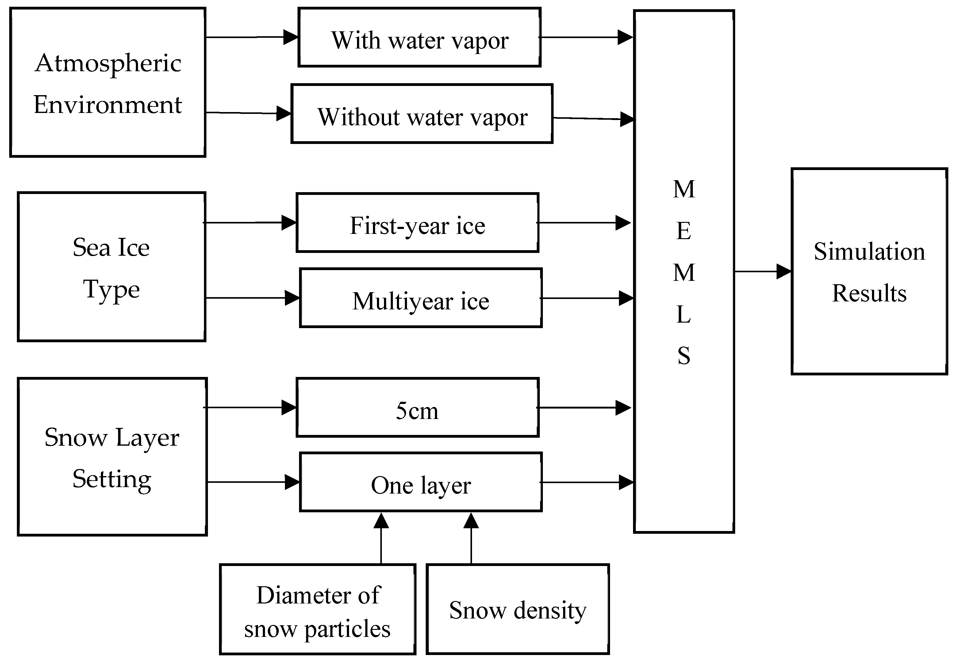
We also considered two types of snow layers, snow with only one layer and snow layered every 5 cm. In the former case, the density and diameter of particles were varied, while for the latter we used the same values referring to Tonboe et al. [57], because the in situ snow density profile data on Arctic sea ice is scarce, and there is not enough to support the simulation. The simulation process with different parameter settings is illustrated in Figure 1.

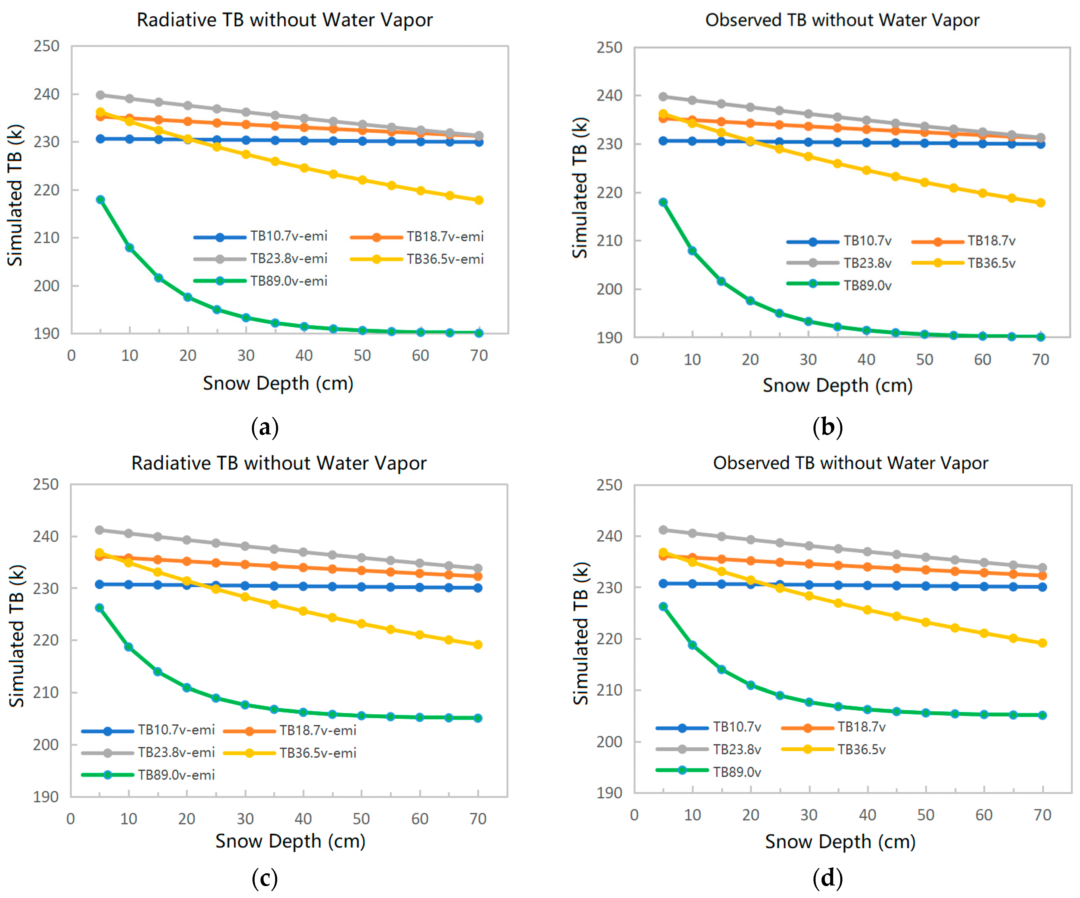
First, the influence of the atmosphere on the TBs was analyzed by simulating the TBs with and without water vapor in the atmosphere. The internal radiant TB from snow and the observed TBs (including the reflected downward radiation from the atmosphere) are shown in Figure 2.

It was found that there is no difference between the radiant TB from snow and the observed TB, regardless of whether water vapor is present in the atmosphere. It can be concluded that the influence of downward atmospheric radiation can be discounted. Comparing the TBs in conditions with and without water vapor, it was found that, except for the channels at 23.8 GHz and 89 GHz, the TBs are very similar in both cases on the other channels. Thus, water vapor influences the TBs at 23.8 GHz and 89 GHz, but has no effect on the observed TBs from other channels. Therefore, when using MEMLS for sensitivity analysis later, we do not account for downward atmospheric radiation, and uniformly use the observed TB without water vapor.

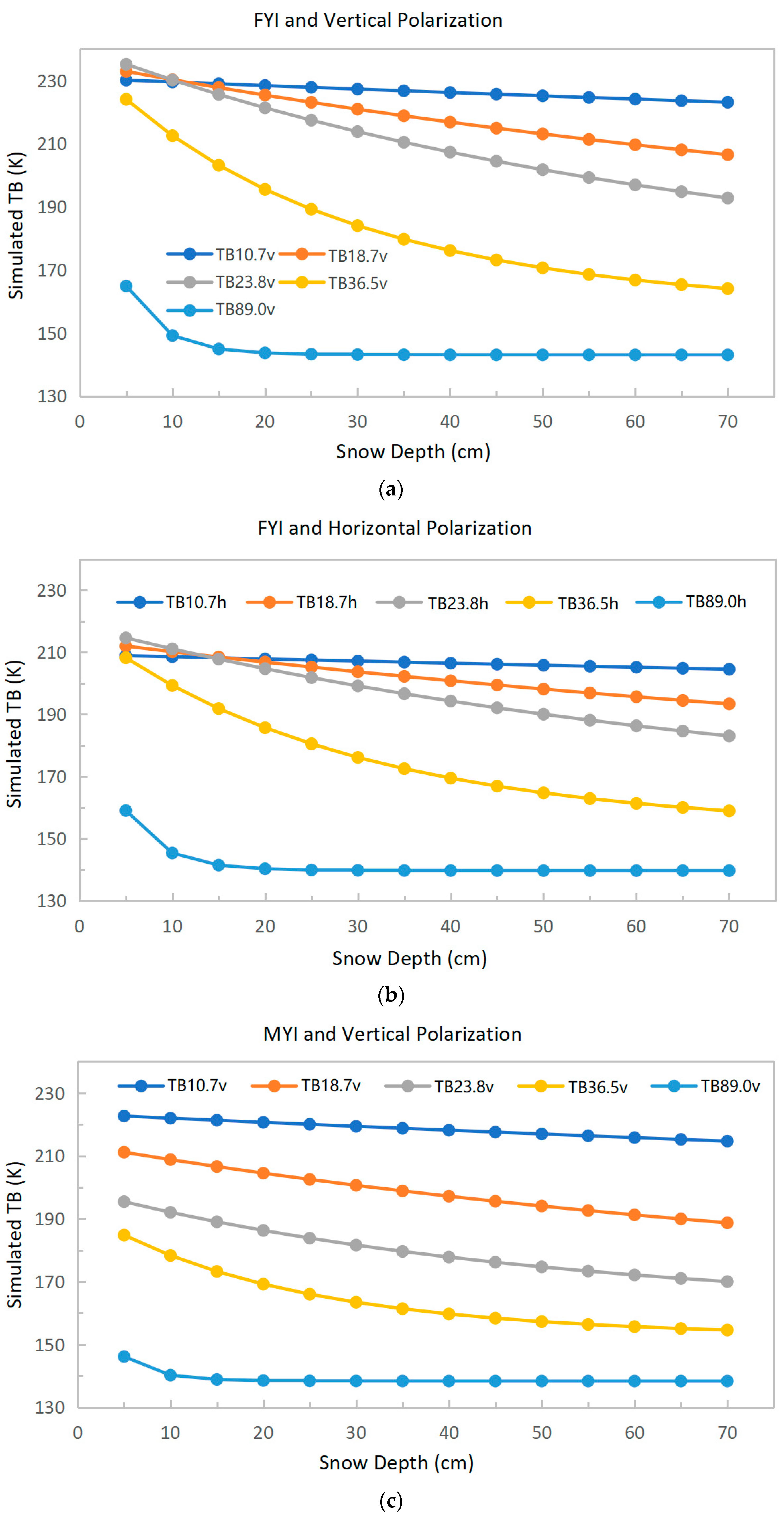
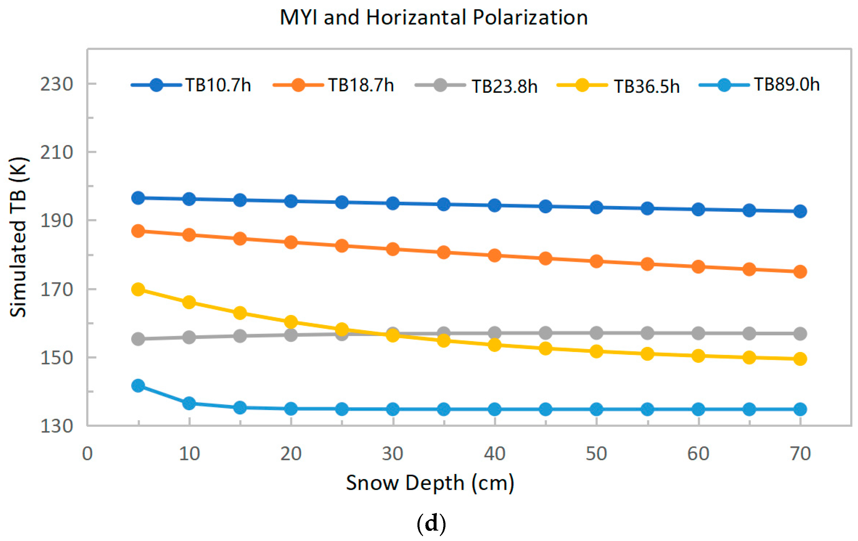
We then conducted the simulation for single-layer snow. In this condition, we set the snow density to 300 kg/m³ and the particle diameter to 1.5 mm as an example. The simulation results are shown in Figure 3.

It can be seen that the observed TBs from vertical channels on FYI decrease as the snow depth increases, and the higher the frequency is, the greater the variation of TBs is, except for 89 GHz. As the snow depth changes from 5 to 70 cm, T_B(10.7 V), T_B(18.7 V), and T_B(36.5 V) decrease by 7 K, 26 K, and 60 K, respectively (T_B denotes TB; V denotes vertical polarization); when the snow is thinner, the attenuation of T_B(89 V) is obvious. As the snow depth increases, the attenuation tends to saturate, and the rate of TB change decreases significantly. The results from the horizontal channels are similar to the above. The main difference is that the rate of changes in TBs is lower than for vertical polarization. The simulations on MYI are also similar to those on FYI. As the snow depth changes from 5 to 70 cm, T_B(10.7 V), T_B(18.7 V), and T_B(36.5 V) decrease by 8 K, 22 K, and 30 K, respectively.

Third, we analyze the snow depth changes with the gradient ratios in different channels. The gradient ratio is defined as follows [53]:

$$\mathrm{GR}\left(f1p1/f2p2\right)=\frac{{\mathrm{T}}_{\mathrm{B}}\left(f2,p2\right)-{\mathrm{T}}_{\mathrm{B}}\left(f1,p1\right)}{{\mathrm{T}}_{\mathrm{B}}\left(f2,p2\right)+{\mathrm{T}}_{\mathrm{B}}\left(f1,p1\right)}$$

(1)

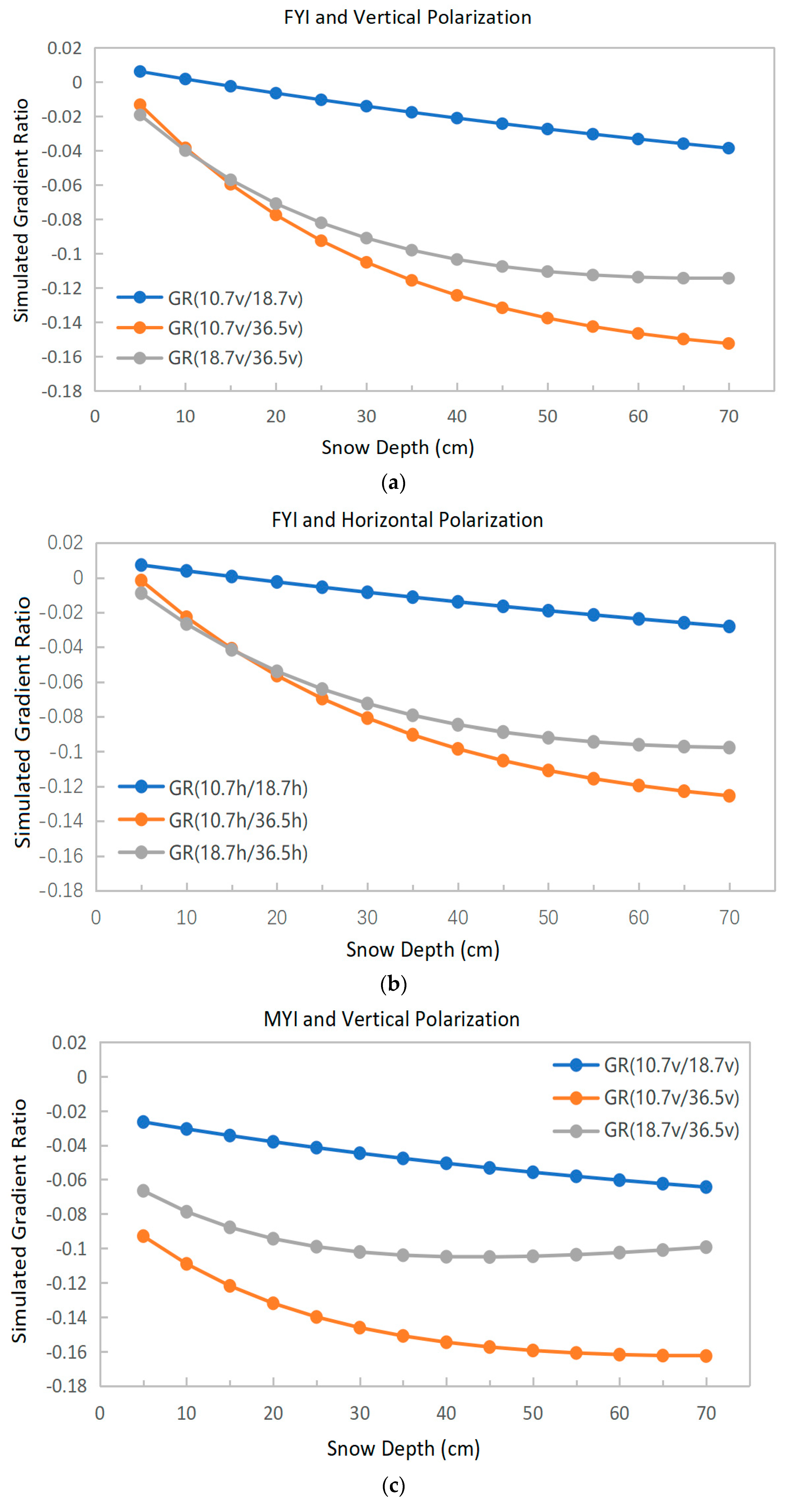
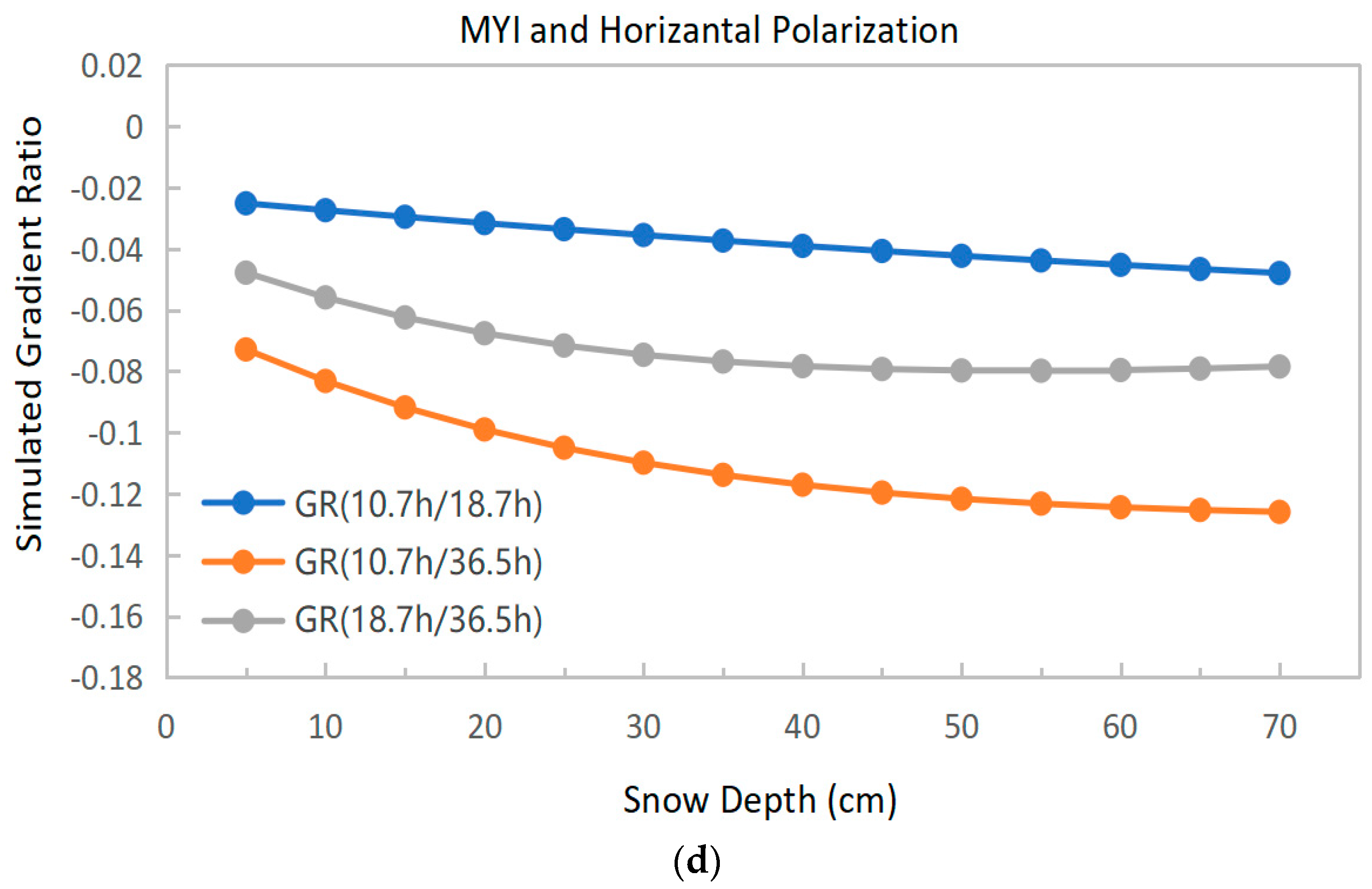
where GR is the gradient ratio, and T_B(f,p) is the TB at frequency f with polarization p (horizontal or vertical). The changes in GRs with snow depth are shown in Figure 4.

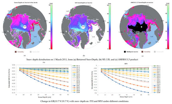
It can be seen from Figure 4 that, for both FYI and MYI, the simulated GR(10.7 V/18.7 V) and GR(10.7 V/36.5 V) decrease as the snow depth increases. The difference is that the former has a linear relationship with respect to snow depth, whereas the latter exhibits a decreasing rate of change as the snow becomes deeper. GR(18.7 V/36.5 V) decreases as the snow depth increases in FYI and tends to saturate when the snow depth is above 50 cm. However, for MYI, it no longer drops once the snow depth is around 30 cm. This is consistent with the conclusion of Markus [23] that the GR can be used to calculate the snow depth on FYI below 50 cm, but cannot be used to retrieve the snow depth on MYI. The results for horizontal polarization are similar to those for vertical polarization. The main difference is that the gradient ratio changes more slowly with the snow depth than in the case of vertical polarization.

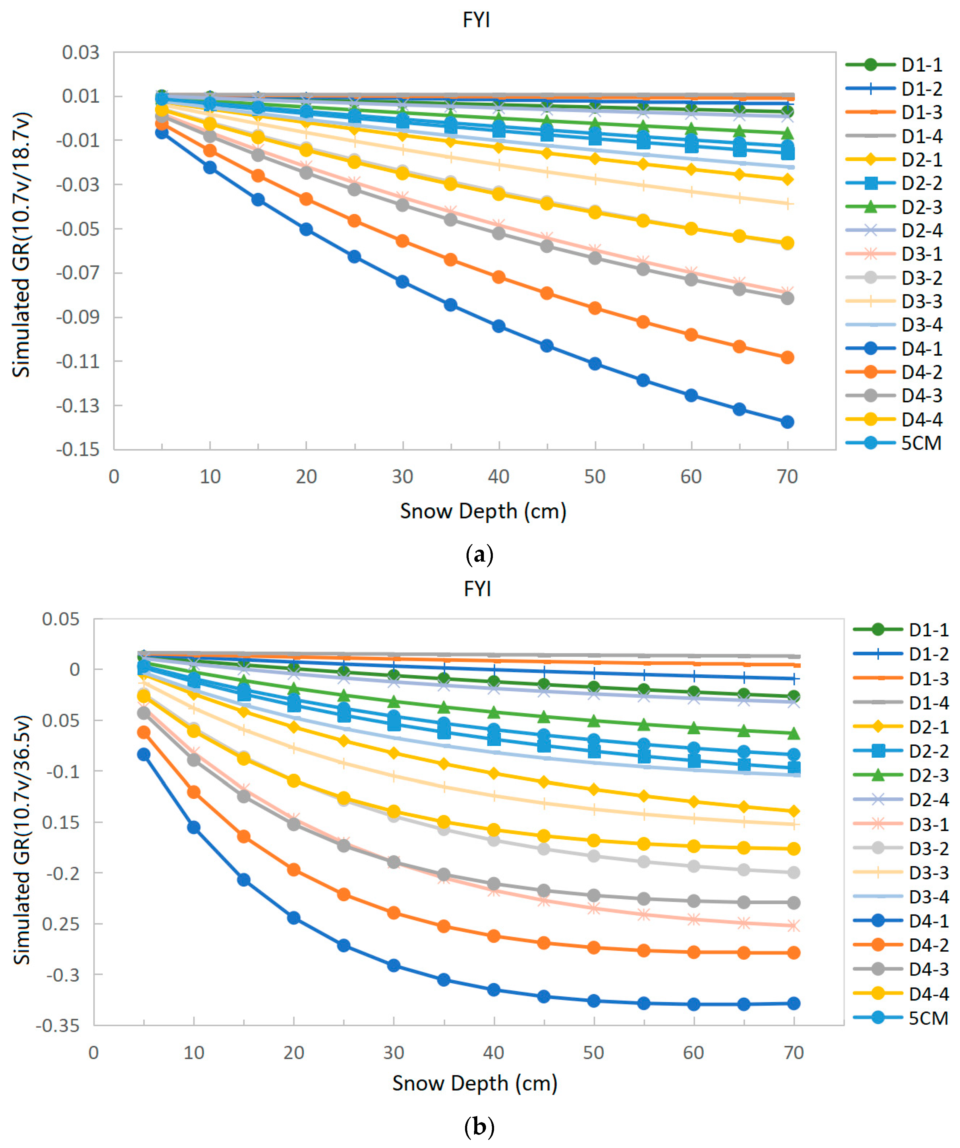
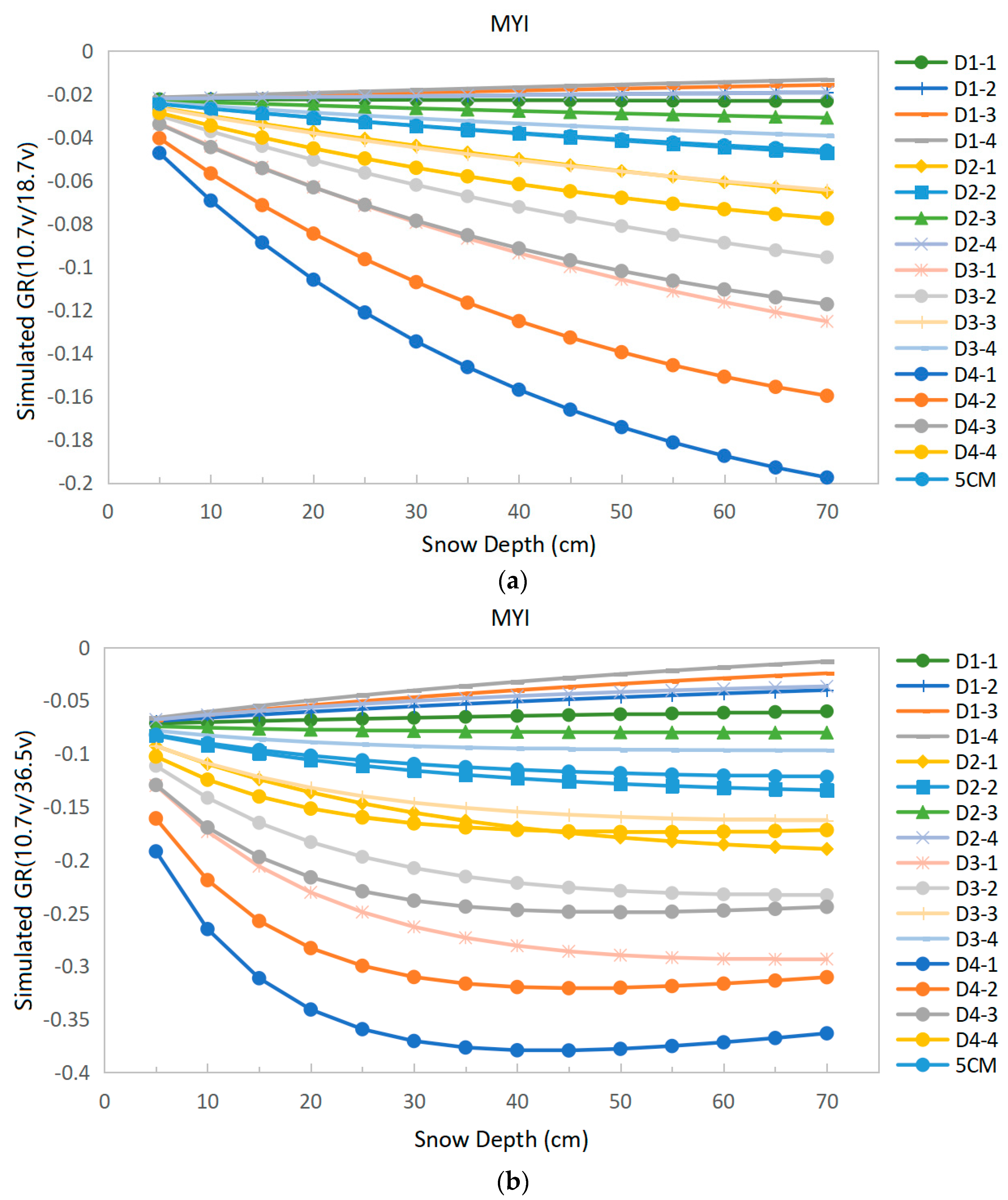
Based on the simulations above, we compared GR(10.7 V/18.7 V) and GR(10.7 V/36.5 V) under different densities, correlation lengths, and layering methods. The vertical polarized GRs on FYI are shown in Figure 5.

“D1–1” to “D4–4” represent different snow conditions in the single layer simulations, as listed in

Table 2. Settings of snow density, particle size, and correlation length in single layer simulation.

Code	FYI			MYI
	Particle Size (mm)	Snow Density (kg/m3)	Correlation Length (mm)	Particle Size (mm)	Snow Density (kg/m3)	Correlation Length (mm)
D1–1	0.5	200	0.078	0.5	200	0.078
D1–2	0.5	250	0.073	0.5	260	0.072
D1–3	0.5	300	0.067	0.5	330	0.064
D1–4	0.5	350	0.062	0.5	400	0.056
D2–1	1.0	200	0.156	1.2	200	0.188
D2–2	1.0	250	0.145	1.2	260	0.172
D2–3	1.0	300	0.135	1.2	330	0.154
D2–4	1.0	350	0.124	1.2	400	0.135
D3–1	1.5	200	0.235	1.8	200	0.281
D3–2	1.5	250	0.218	1.8	260	0.258
D3–3	1.5	300	0.202	1.8	330	0.230
D3–4	1.5	350	0.185	1.8	400	0.203
D4–1	2.0	200	0.313	2.5	200	0.390
D4–2	2.0	250	0.291	2.5	260	0.358
D4–3	2.0	300	0.269	2.5	330	0.320
D4–4	2.0	350	0.247	2.5	400	0.282
5 cm	1.2	300	0.15	1.8	350	0.2

, whereas “5 cm” denotes the simulations with snow layered every 5 cm.

Figure 5 shows that on FYI, GR(10.7 V/18.7 V) decreases near-linearly with increasing snow depth in various environments, and decreases faster with increasing particle size. When the particle size is constant, a smaller density results in a faster decrease inGR. Meanwhile, GR(10.7 V/36.5 V) decreases linearly with the increase in snow depth for small particle size. When the snow depth is less than about 50 cm and the particle size increases, the ratio decreases as the snow depth increases, and then becomes saturated. This is mainly because, as the particle size of snow becomes larger, the scattering of microwave signals by snow gradually increases, which leads to faster changes in TBs with snow depth. Because the scattering of microwave signals is greater at high frequency than at low frequency, the signal attenuation becomes very fast as the particle size increases and becomes saturated at a certain snow depth, which will result in GRs that no longer decrease as the snow depth increases. In some extreme cases, the GR will even increase as snow depth increases when the TB change at high frequency is lower than that at low frequency.

The case for MYI is shown in Figure 6.

Similar to the case of FYI, GR(10.7 V/18.7 V) decreases almost linearly with increasing snow depth, except in extreme cases. With increasing particle size, the GRs gradually increase. GR(10.7 V/36.5 V) also decreases with increasing snow depth when the snow depths are below 30 cm and then remains fairly constant. When the snow particle size is large, this gradient ratio increases with snow depth.

To further analyze the relationship between TBs (GRs) and snow depths, correlation coefficients between them are presented in

Table 3. Correlation coefficients between TBs (GRs) and snow depths.

Parameter	Correlation Coefficient (FYI)	Correlation Coefficient (MYI)
TB(10.7 V)	−0.764	−0.529
TB(18.7 V)	−0.879	−0.524
TB(36.5 V)	−0.956	−0.355
GR(10.7 V/18.7 V)	−0.993	−0.523
GR(10.7 V/36.5 V)	−0.955	−0.323

.

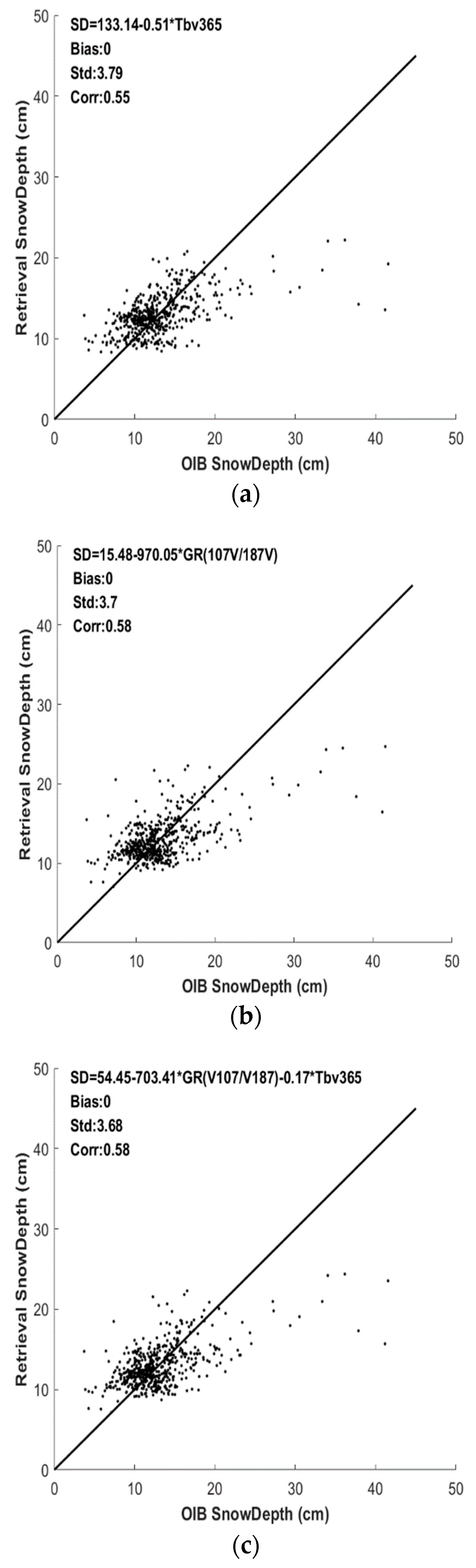
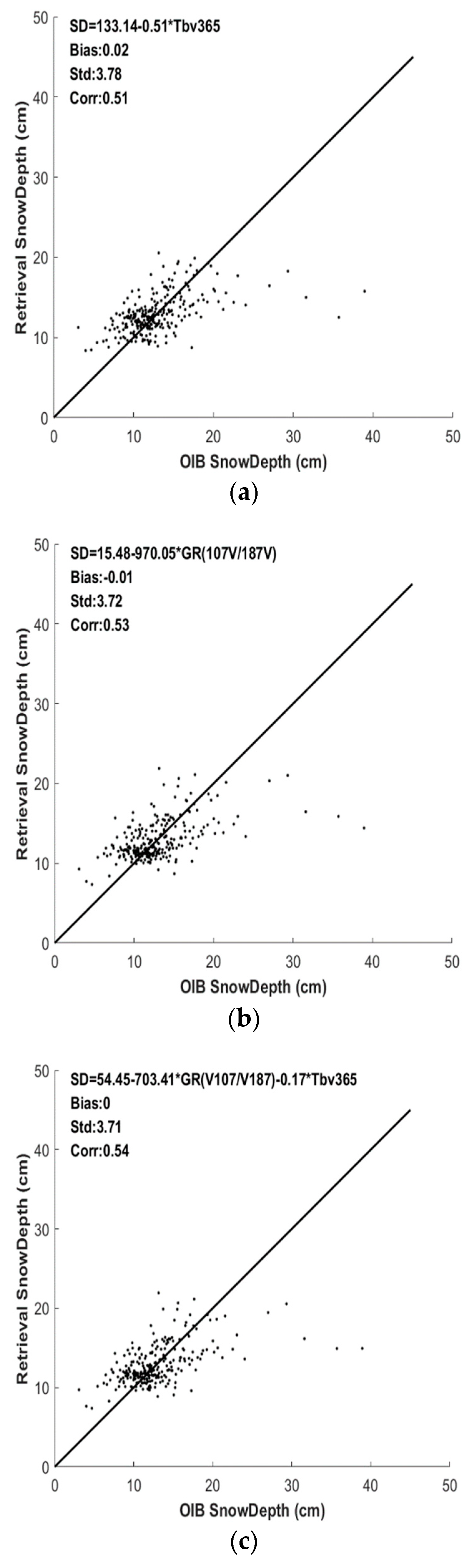
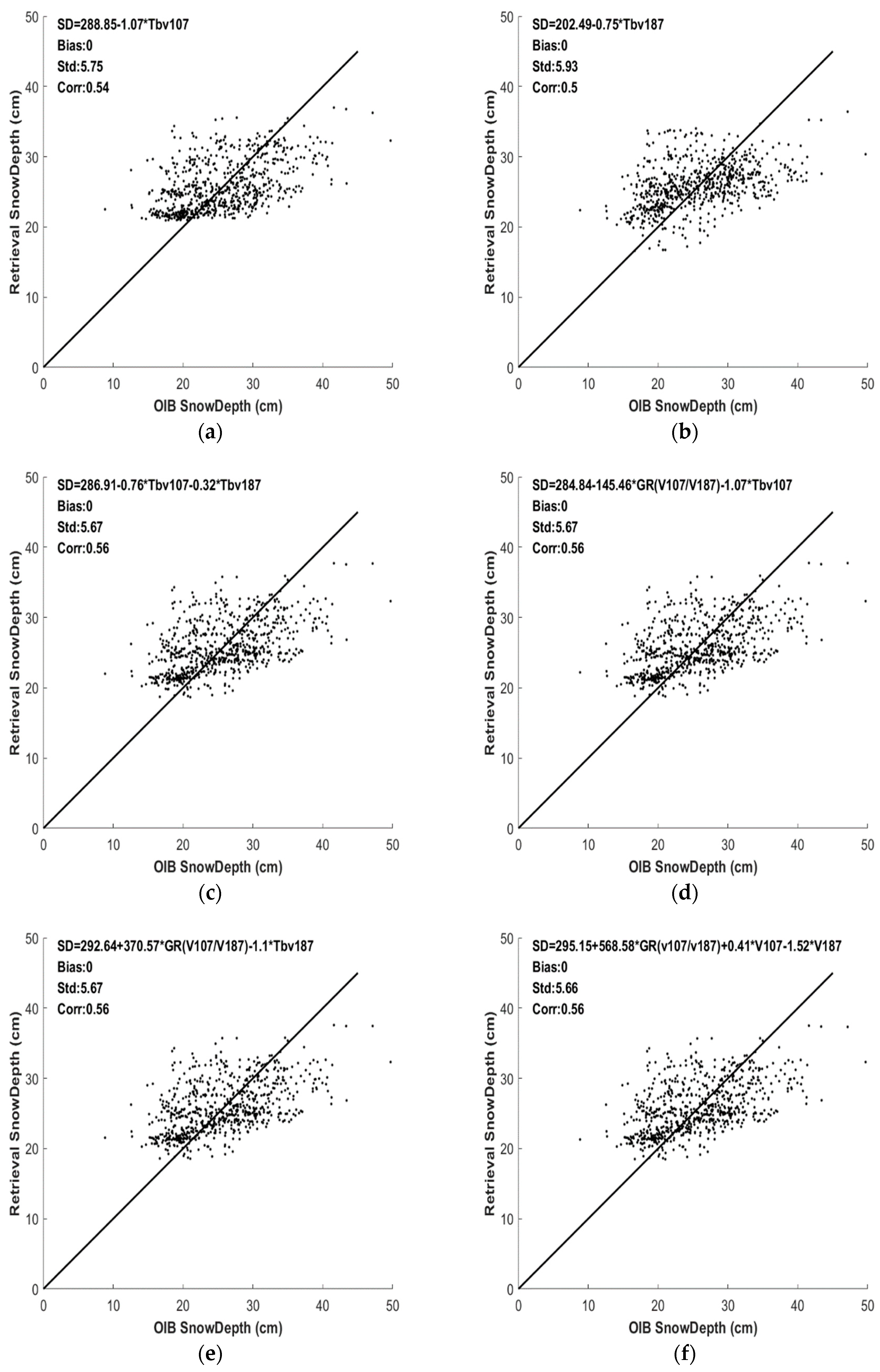
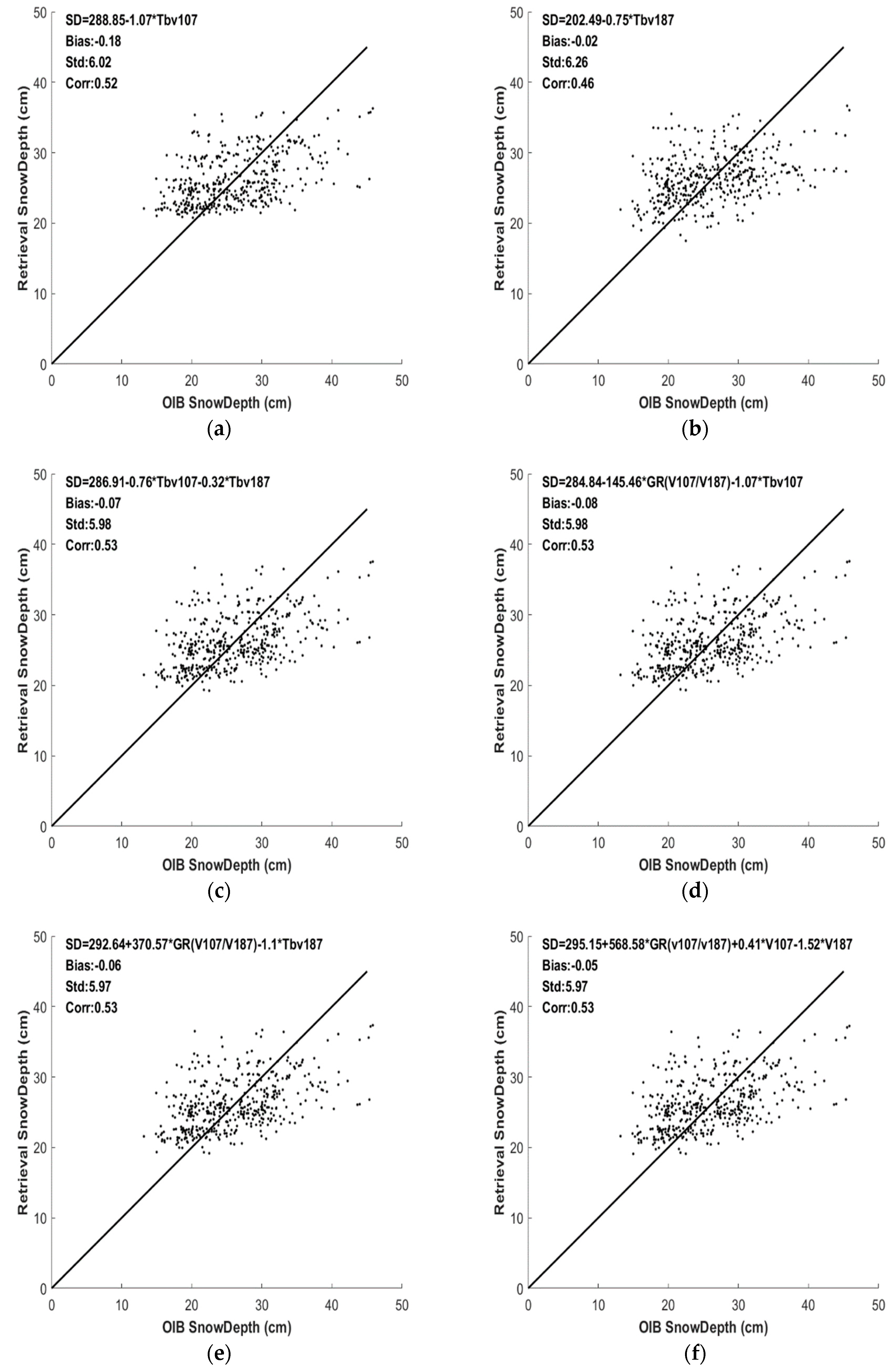
Based on the sensitivity and correlation analyses above, the GR(10.7 V/18.7 V) and TB(36.5 V) are the best parameters for snow depth retrieval on FYI, whereas TB(10.7 V), TB(18.7 V), and GR(10.7 V/18.7 V) are best for MYI.

4. Snow Depth Retrieval

4.1. Algorithm Development

Based on the analysis above, snow depth retrieval on Arctic sea ice is explored using FY3B/MWRI TB and OIB snow depth data. As the OIB IDCSI4 data and MWRI have a three-year overlap time (2011–2013), we chose data from 2012 and 2013 to develop the retrieval algorithm and used 2011 data for algorithm verification.

4.1.1. Data Preprocessing

First, datasets were preprocessed, including deleting invalid data, re-gridding the SIT data, and averaging and projecting TBs from MWRI and snow depths from OIB. Second, we matched the TBs and snow depths. Afterwards, according to SIT data, we classified them into two datasets for FYI and MYI, separately. Two-thirds of each dataset were used for algorithm development, and one-third was for calibration. The numbers of the match up data for algorithm development and calibration are listed in

Table 4. The amount of snow depth data for algorithm development and verification.

Type of Data	FYI	MYI
Algorithm development	508	814
Algorithm calibration	254	407
Total	762	1221

. Figure 7 and Figure 8 show histograms of snow depths for different usage.

On FYI, the average snow depth of the algorithm development is 12.98 cm, and the Std is 4.54 cm; for the calibration dataset, the average snow depth is 12.91 cm, and the Std is 4.39 cm. Meanwhile, on MYI, the average value of the algorithm development data is 28.75 cm, and the Std is 6.64 cm; for the calibration dataset, the corresponding values are 28.69 cm and 6.56 cm. The locations of OIB data in 2012 and 2013 are shown in Figure 9.

4.1.2. Algorithm Development

According to Section 3, we selected GR(10.7 V/18.7 V) and T_B(36.5 V) for snow depth retrieval on FYI, and T_B(10.7 V), T_B(18.7 V), and GR(10.7 V/18.7 V) for MYI. The sea ice concentrations were calculated using the Arctic Radiation and Turbulence Interaction Study Sea Ice (ASI) algorithm with improved tie points [58].

• FYI

According to our sensitivity analysis, the relations between TBs (GRs) and the snow depth on FYI are approximately linear. Therefore, the possible equations for the retrieval algorithm are as follows:

SD = a + b* TB(36.5 V)

(2)

SD = a + b* GR(10.7 V/18.7 V)

(3)

SD = a + b*GR(10.7 V/18.7 V) + c* T_B(36.5 V)

(4)

where SD refers to snow depth in cm; a, b, and c are algorithm coefficients calculated by the development dataset. The fitting results of different coefficients for Equations (2)–(4) are shown in Figure 10.

The fitting results show that the three equations perform similarly. They were then verified by using the TBs from the calibration data to calculate the snow depths with different retrieval algorithms, and the results were compared with the OIB snow depths from the calibration data shown in Figure 11.

Table 5. Statistics of the calibration results on FYI.

Equation	Bias (cm)	Std (cm)	RMSE (cm)	Correlation Coefficient
2	0.02	3.78	3.78	0.51
3	−0.01	3.72	3.72	0.53
4	0	3.71	3.71	0.54

presents the statistics of the calibration.

Based on Figure 11 and Table 5, we can conclude that the algorithm corresponding to Equation (4) performs the best. As shown in Figure 10 and Figure 11, there is poor performance for all methods in relatively deep snow. The main reason is that data larger than 20 cm in the development dataset are very rare, so the algorithm can obtain better results at low snow depth values than at high ones. When the field snow depth data, especially the deep snow data on FYI, are sufficient, the algorithm can later be upgraded. In this study, according to Figure 11 and Table 5, the retrieval algorithm for FYI is

SD = 54.45 − 703.41*GR(10.7 V/18.7 V) − 0.17* T_B(36.5 V).

(5)

• MYI

As for FYI, the algorithms for MYI are considered as follows.

SD = a + b* T_B(10.7 V)

(6)

SD = a + b* T_B(18.7 V)

(7)

SD = a + b* T_B(10.7 V) + c* T_B(18.7 V)

(8)

SD = a + b*GR(10.7 V/18.7 V) + c* T_B(10.7 V)

(9)

SD = a + b*GR(10.7 V/18.7 V) + c* T_B(18.7 V)

(10)

SD = a + b*GR(10.7 V/18.7 V) + c* T_B(10.7 V) + d* T_B(18.7 V)

(11)

The fitting results, using match up data for algorithm development, are shown in Figure 12.

Similar to the algorithm development for FYI, the above algorithms were used to calculate the snow depths corresponding to the TBs from calibration dataset. The retrieved snow depths were then compared with the snow depths from OIB. The results are shown in Figure 13.

The calibration results of each algorithm are listed in

Table 6. Statistics of calibration results on MYI.

Equation	Bias (cm)	Std (cm)	RMSE (cm)	Correlation Coefficient
6	−0.18	6.02	6.02	0.52
7	−0.02	6.26	6.26	0.46
8	−0.07	5.98	5.98	0.53
9	−0.08	5.98	5.98	0.53
10	−0.06	5.97	5.97	0.53
11	−0.05	5.97	5.97	0.53

.

Figure 13 and Table 6 indicate that a combination of GR(10.7 V/18.7 V), T_B(10.7 V), and T_B(18.7 V) yields the highest accuracy. Therefore, the snow depth retrieval algorithm on MYI is

SD = 295.15 + 568.58*GR(10.7 V/18.7 V) + 0.41*T_B(10.7 V) − 1.52*T_B(18.7 V).

(12)

4.2. Comparison and Verification

Based on the retrieval algorithms, we calculated daily Arctic snow depths using FY3B/MWRI TBs from January–May 2011. It should be mentioned that, when determining the sea ice type in the retrieval process, the intensity ratio method was used to distinguish the FYI and the MYI [59]. To eliminate the influence of grain size uncertainties, density variations, and sporadic weather effects, three-day averaged snow depths were used. In this process, we set the melting flags and variable flags on points where the snow was melted or the snow depth had great variation over three days. Figure 14 shows the snow depth distribution on 3 January 2011, as an example.

This figure denotes the averaged snow depth for three days from 1–3 January 2011. To eliminate the influence of land on the retrieval, we removed the data close to land using a 3 × 3 grid mask.

4.2.1. Comparison with Other Datasets

To evaluate the algorithm, a comparative analysis was conducted against three snow depth datasets. The time coverage of SD_UB is from November to April/May, and the data for MYI began on 1 March each year. Considering that, we compared the snow depths on the FYI from January–April 2011 in the three datasets, and on MYI in two datasets, the snow depths of this study (RSD) and SD_UB from March to April 2011 (there are no SD_UB data after 24 April 2011). Finally, we had 111 days for comparison on FYI and 55 days on MYI. As an example, the snow depths from the three datasets on 1 March 2011, are shown in Figure 15.

We can see in Figure 15 that the snow depths retrieved in this study (RSD) are lower than those of the other two datasets on FYI, but higher than that of SD_UB on MYI. The differences are shown in Figure 16.

On FYI, the snow depth differences between RSD and AMSR-E are the smallest, less than 5 cm in most areas. The differences between RSD and SD_UB are the clearest—5–10 cm lower in RSD than in SD_UB on average. The snow depths of AMSR-E are also lower than those of SD_UB, while for MYI, the snow depths of RSD are lower than those of SD_UB, and in many areas, the differences are very similar to those with respect to FYI.

We then compared the three datasets monthly to see if there were monthly changes. The statistical results are presented in

Table 7. Statistics of snow depth differences (RSD minus AMSR-E).

Month	Number of Matchup Data	Bias (cm)	Std (cm)	RMSE (cm)
1	1243520	−1.59	4.16	4.45
2	1316703	−1.75	4.03	4.39
3	1509787	−2.80	4.26	5.10
4	1102124	−4.64	4.76	6.65
All	5172134	−2.63	3.47	4.35

and

Table 8. Statistics of snow depth differences (RSD minus SD_UB).

Area	Month	Number of Matchup Data	Bias (cm)	Std (cm)	RMSE (cm)
FYI	1	1243520	−7.06	3.43	7.85
	2	1316703	−6.56	3.52	7.44
	3	1509787	−6.64	3.48	7.50
	4	1102124	−6.35	3.37	7.19
	All	5172134	−6.66	4.44	8.00
FYI and MYI	3	1977770	−6.34	3.58	7.28
	4	1424654	−6.36	3.38	7.30
	All	3402424	−6.35	3.50	7.25

.

It appears that the snow depths from RSD are lower than those from AMSR-E and SD_UB. The bias between RSD and the AMSR-E product ranges from −4.64 to −1.59 cm, and the Std is from 4.03 to 4.76 cm. The bias is relatively small in January and February compared with that in March and April, and the overall deviation is −2.63 cm. When compared with the SD_UB data, the bias and Std are relatively concentrated on both FYI and the entire sea ice. The bias on FYI is −6.66 cm, while the Std is 4.44 cm. For all datasets, the bias is −6.35 cm, and the Std is 3.5 cm. The results show that the retrieval algorithm presented in this study is closer to the AMSR-E product on FYI, and the difference between RSD and SD_UB changes little from FYI to the entire sea ice.

The main reasons for the differences between the snow depths from RSD and other products are as follows: (1) differences caused by different retrieval algorithms of snow depth. The three datasets are produced by three algorithms using different channels and forms, which will lead to snow depth differences. (2) Differences caused by different sensors. This study is based on FY3B/MWRI TBs, while the other two datasets are based on Aqua/AMSR-E data. Differences in TBs may lead to snow depth differences. The in-orbit calibration and quality evaluation of FY3B/MWRI conducted by Yang et al. [30,60] indicate that the calibration accuracy of the sensor meets the design requirements, that is, the high-frequency channel reaches 2.5 K and the low-frequency channel 2 K. According to Chen [61], the TB differences between MWRI and AMSR-E in different channels can be up to 4 K, and for the vertical channels used in this study, the biases are about 3 K with a Std of 3 K. According to our sensitivity analysis, a 6 K difference in TB on low-frequency channels can lead to snow depth differences of up to 5 cm. (3) Snow depth differences induced by different sea ice classification methods. In AMSR-E products, the MYI is determined by setting the threshold of GR(18.7 V/36.5 V) to −0.02; SD_UB uses the SIT product to identify MYI. In this study, we explored an intensity ratio method to identify ice type based on the TB. A dynamic threshold was also adopted. (4) Errors produced by different sea ice concentrations. In this study, we used the ASI algorithm with improved tie points; SD_UB also uses the ASI algorithm, whereas the AMSR-E product applies the NT2 algorithm. From the sensitivity analysis above, a 10% error in sea ice concentration would produce a snow depth error of up to 5 cm in areas of low sea ice concentrations, thus leading to the difference among the three snow depth datasets.

4.2.2. Algorithm Verification

To evaluate the algorithm accurately, we verified the three groups of snow depths against the OIB data from 2011 for FYI and MYI conditions. Histograms and spatial distributions of the snow depth data for verification are shown in Figure 17 and Figure 18, respectively.

After data preprocessing, we obtained 42 matchup data for FYI and 784 for MYI. The average snow depth on the FYI is 12.19 cm, and the Std is 4.41 cm; the average snow depth on MYI is 23.68 cm, with a Std of 5.74 cm. The verification results are presented in

Table 9. Algorithm verification results.

Sea Ice Type	Data Set Minus OIB	Bias (cm)	Std (cm)	RMSE (cm)	Mean Relative Error (%)
First-year	AMSR-E	4.54	2.80	5.33	43.58
	SD_UB	8.29	3.00	8.82	81.62
	RSD	2.89	2.60	3.89	31.02
Multiyear	SD_UB	7.59	4.71	8.93	36.29
	RSD	1.44	4.53	4.75	18.59

.

Table 9 shows that the biases of RSD on FYI and MYI are 2.89 and 1.44 cm, respectively, with Stds of 2.6 and 4.53 cm. These statistics are better than those corresponding to the other two data products.

A comparison of the three datasets minus the OIB data is shown in Figure 19.

The difference between RSD and OIB on FYI tends to be less than 5 cm, which accounts for 86% of the total data. It accounts for only 9% of the SD_UB data and 67% of the AMSR-E data, which is consistent with previous research [17,20].

For MYI, histograms of the snow depth differences are displayed in Figure 20.

The differences between RSD and OIB on MYI tend to be within ±5 cm, accounting for 71% of the total data; the differences between SD_UB and OIB are up to 8 cm, similar to those reported by Braakmann-Folgmann and Donlon [28].

The following issues may cause differences between RSD and OIB: (1) Spatial and temporal differences between OIB and MWRI data. First, the OIB data are observed on a certain point and certain time, whereas the snow depths from MWRI are calculated from daily average TB data. The time difference may lead to different results. Second, the grid resolution of MWRI data is 12.5 km, whereas the OIB is 40 m. Insufficient OIB data may introduce errors during processing. (2) Limited data for algorithm development, which will lead to errors. The number of OIB datasets is limited and they are mainly collected from the Beaufort Sea and Central Arctic region, which may introduce errors when using them to develop an algorithm for the entire Arctic. (3) Retrieval errors caused by errors in sea ice concentration. (4) OIB systematic errors. Kurtz et al. [62] showed that the average error in the snow depths from OIB data is about 5.7 cm, which will induce errors in snow depth retrieval. (5) Retrieval errors caused by different sea ice and snow conditions. The sensitivity analysis reported in this study indicated that different snow particle sizes and snow densities will influence the scattering of microwave signals. The algorithm developed herein deals with snow depth retrieval only under the general state, and may induce errors when extreme conditions occur. (6) Errors caused by sea ice classification. As the physical properties of FYI and MYI are different, this study adopts different retrieval algorithms for them. Misclassification of sea ice type will lead to misuse of the algorithm and result in retrieval errors.

5. Conclusions

Based on the TBs from the FY3B/MWRI, a study of snow depth retrieval in the Arctic was conducted for both first-year and multiyear ice. Starting from the physical process of microwave signal transmission in ice, snow, and the atmosphere, the influence of snow depth variations on surface observed TBs was analyzed, along with their correlation based on radiative transfer theory. This sensitivity analysis was based on the physical simulation of the microwave transmission process, which is more reasonable and credible. On this basis, the optimal channel combinations and forms for snow depth retrieval were proposed on Arctic sea ice using TBs from the FY3B/MWRI. An algorithm for snow depth retrieval was then developed using TBs from the FY3B/MWRI and snow depths from OIB, on both FYI and MYI in the Arctic. Verification results indicated that the bias and Std of the algorithm developed in this study were 2.89 and 2.6 cm, respectively, on FYI, and 1.44 and 4.53 cm, respectively, on MYI. It can be concluded that the snow depths derived herein are effective and in good agreement with OIB data. The proposed algorithm was proven useful for the effective retrieval of snow depth on sea ice from FY3B/MWRI TBs in the Arctic. Importantly, this study provides the first algorithm of snow depths from MWRI that realizes the full coverage of the Arctic sea ice.

Of course, the algorithm still has some limitations. For example, due to the strong absorption of microwave radiation by liquid water, the microwave signal cannot penetrate wet snow. Therefore, the snow depth retrieval using microwave radiometers, including the algorithm in this study, can only calculate the dry snow. A multi sensor combination method to calculate wet snow depth may be taken into account in a future study. Moreover, we will call for more attention to the continuous collection of field snow depth data, including snow profiles for snow density and snow grain size, to further simulate the effect of snow depth on observed TBs in various snow profiles, together with deep snow data on FYI and MYI, e.g., from the MOSAiC (Multidisciplinary drifting Observatory for the Study of Arctic Climate), to ensure sufficient snow depth data in all numerical ranges. As analysis of the sensitivity of MWRI TBs to snow depths is decided by physical modeling, it does not depend on field datasets. With the increase of in situ snow depth data, the algorithm can be upgraded, but the channels and parameters will remain unchanged.