Deep Learning Based Sea Ice Classification with Gaofen-3 Fully Polarimetric SAR Data

Abstract

In this paper, the performance of C-band synthetic aperture radar (SAR) Gaofen-3 (GF-3) quad-polarization Stripmap (QPS) data is assessed for classifying late spring and summer sea ice types. The investigation is based on 18 scenes of GF-3 QPS data acquired in the Arctic Ocean in 2017. In this study, floe ice (FI), brash ice (BI) between floes and open water (OW, ice-free area) were classified based on a mini sea ice residual convolutional network, which we call MSI-ResNet. While investigating the optimal patch size for MSI-ResNet, we found that, as the patch size continues to grow, the classification accuracy first increases and then decreases. A patch size of 31 × 31 was found to achieve the best performance. The performance of classification using different polarization combinations from the QPS data was also assessed. The vertical-vertical (VV) polarization input overestimates the FI category while incorrectly identifying most of the BI as FI. The VH polarization produces a synchronous improvement in FI, BI, and OW discrimination, with a higher overall accuracy and kappa coefficient (91.09% and 0.85, respectively) than the VV polarization (83.37% and 0.70, respectively). The combination of VV and vertical-horizontal (VH) polarizations presents a modest precision improvement for BI and OW together with a slight overestimation for FI. With VV, VH, and horizontal-horizontal (HH) polarization data as the inputs, the user’s accuracy improves to 95.12%, 93.42%, and 95.17% for FI, BI, and OW, respectively. The accuracy was assessed against visual interpretation of the sea ice classes in the images using a stratified sampling method. The application of the MSI-ResNet method to data covering the Beaufort Sea and the north of the Severnaya Zemlya archipelago was found to achieve a high overall accuracy (kappa) of 94.62% (±0.92) and 94.23% (±0.90), respectively. This is similar to the classification accuracy obtained in the Fram Strait. From the results of this study, it is shown that the MSI-ResNet method performs better than the classical support vector machine (SVM) classifier for sea ice discrimination. The GF-3 QPS mode data also show more details in discriminating scattered sea ice floes than the coincident Sentinel-1A Extra Wide (EW) swath mode data.

1. Introduction

Polar sea ice is a sensitive indicator of global climate changes. Information about sea ice type is also important for ship navigation and climate change prediction in polar regions [1,2,3,4,5]. However, the large extent and harsh environment make most of the polar regions difficult to access and the cost of field investigation remarkably high [6]. Spaceborne remote sensing methods, particularly those using active and passive microwave instruments have proven to be successful in monitoring sea ice. Long-term records of Arctic sea ice monitoring (>40 years) are now available from different operational sources, including the Canadian Ice Service (CIS), the Russian Arctic and Antarctic Research Institute (AARI), the Norwegian Ice Service (NIS), and the U.S. National Ice Center (NIC).

Synthetic aperture radar (SAR) has proven to be suitable for monitoring polar sea ice because it is independent of sunlight and atmospheric influences such as clouds and water vapor [7,8,9]. As the imaging mechanism is triggered by surface roughness and subsurface physical properties, SAR can be used to distinguish the different types of sea ice. A few milestones among the SAR systems that have been used to monitor and research Arctic sea ice are NASA’s SeaSAT mission, the series of satellites operated by the European Space Agency (ESA) (the European Remote Sensing, ENVISAT, and Sentinel-1 systems), the Japan Aerospace Exploration Agency (JAXA) Advanced Land Observing Satellite/Phased Array type L-band Synthetic Aperture Radar (ALOS PALSAR) systems, the German Aerospace Center (DLR) TerraSAR systems, and the Canadian Space Agency (CSA) RADARSAT systems.

Many studies of sea ice classification using polarimetric SAR data have been conducted as polarized data hold more information about the ice surface. According to Gill et al. [10], the authors explored the potential of polarimetric parameters and used ground truth data to estimate sea ice classification accuracy based on the maximum likelihood classifier. They found that the accuracy increased when more uncorrelated polarimetric parameters were used. By using the parameters of ${\mathsf{\sigma }}_{\mathrm{vv}}^0$, entropy and ${\mathsf{\sigma }}_{\mathrm{hv}}^0$, the accuracies for open water (OW), smooth first-year ice (SFYI), rough first-year ice (RFYI), and deformed first-year ice (DFYI) were 96.72%, 96.58%, 67.44%, and 95.58%, respectively. Moen et al. [11] used three consecutive RADARSAT-2 (RS-2) scenes to investigate the robustness of polarimetric SAR data for sea ice classification under slightly varying winter environmental conditions based on a supervised classification method with unsupervised automatic segmentation and labeling of the scene as a reference. This study discriminated between seven sea ice types and found that scenes with similar incidence angles produced reasonable results. Another study by Ressel et al. [12] examined the performance of an automated sea ice classification algorithm based on polarimetric TerraSAR-X (TS-X) images. By the use of four polarimetric features of the geometric intensity, the scattering diversity, the surface scattering fraction features, and comparison with in situ measurements, the study correctly identified young ice (YI), SFYI, rough first-year and multi-year ice (RFYMYI), multi-year ice (MYI), and OW. The polarimetric features of spaceborne L- (ALOS-2), C- (RS-2), and X- (TS-X) band quad-polarimetric SAR data were evaluated and validated by Singha et al. [13] for sea ice discrimination using an artificial neural network method, obtaining accuracies of 100% and 96.9% for OW and all the sea ice classes, respectively.

The neural network approach has been applied to SAR sea ice classification in previous studies. An unsupervised neural network Learning Vector Quantization method was applied to airborne polarimetric SAR data by Hara et al. [14] to classify sea ice, achieving a total classification accuracy of 77.8%. A pulse-coupled neural networks-based unsupervised method for sea ice classification in the Baltic Sea under dry snow conditions was developed by Karvonen et al. [15] using Radarsat-1 ScanSAR wide mode data. A supervised neural network was also developed by Ressel et al. [16] for TS-X backscatter data using gray level co-occurrence matrix (GLCM) textural features as the inputs. The authors found the classification accuracies for OW, smooth drift ice/smooth fast ice (SDI) and moderately deformed drift ice (MDDI) to be 79.4%, 89.3%, and 94.5% respectively. Song et al. [17] designed a residual convolutional network for sea ice classification called SI-Resnet, using the backscatter from Sentinel-1 SAR Extra Wide (EW) swath mode data in HH polarization, and reported a reasonably high overall classification accuracy and kappa coefficient of 94% and 91.9%, respectively. The ResNet deep learning framework was presented by He et al. [18] for easing the training of networks by reformulating the layers as residual learning functions, with reference to the layer inputs instead of learning unreferenced functions. ResNet V2, which is a refined version of ResNet, was subsequently proposed by He et al. [19] in 2016. To date, ResNet V2 has been found to be one of the most effective deep learning network frameworks for image detection and classification.

Gaofen-3 (GF-3) is a civilian spaceborne SAR satellite developed as part of China’s High-Resolution Earth Observation System Project. GF-3 was launched on 10 August 2016, by the China Academy of Space Technology (CAST). The satellite operates in a sun-synchronous orbit with an orbital altitude of about 755 km, and an in-orbit design life of 8 years. One of its main purposes is monitoring ocean and coastal areas [20]. The nominal resolution of the satellite instruments ranges from 1 to 500 m, and the nominal swath width varies from 10 to 650 km. One of the distinctive features of the GF-3 system is its fully polarimetric imaging capability. GF-3 can acquire fully-polarimetric data in three modes of quad-polarization Stripmap I (QPSI), quad-polarization Stripmap II (QPSII), and wave mode. The former two modes are referred to as QPS mode in this paper. More technical specifications of the sensor can be found in [21,22]. GF-3 SAR data have been used in different marine environment investigations and services, e.g., sea surface wind retrieval [23,24], sea ice detection [25], and ship detection [26,27]. The performance of GF-3 in the observation of intertidal flats, offshore tidal turbulent wakes, and oceanic internal waves has also been evaluated [28]. However, to date, there has been no specific investigation of the polar sea ice classification capabilities of GF-3.

The objective of this study was to investigate the performance of GF-3 full-polarization data for late spring and summer sea ice classification based on the three linear orthogonal polarization backscatter coefficients (${\mathsf{\sigma }}_{\mathrm{vv}}^0$, ${\mathsf{\sigma }}_{\mathrm{hh}}^0$, and ${\mathsf{\sigma }}_{\mathrm{vh}}^0$) from QPS mode data. As residual neural networks have been found to be effective in image recognition [19], we adopted this approach, with some adaptive modifications and developed the MSI-ResNet (where ‘MSI’ means mini sea ice) scheme. This method was found to be effective in discerning between FI, BI, and OW. The optimal patch size for the deep learning scheme was determined, so as to ensure more precise results. The influence of different polarization combinations on sea ice classification was also synthetically explored and analyzed. In addition, in this paper, a comparison between the results from MSI-ResNet and the Support Vector Machine (SVM) classifier [29] for sea ice classification with QPS mode data is presented. Finally, the classification results obtained using GF-3 QPS data are compared with the results obtained from near-coincident Sentinel-1A data using the same MSI-ResNet classifier.

2. Dataset, Preprocessing and Training Data

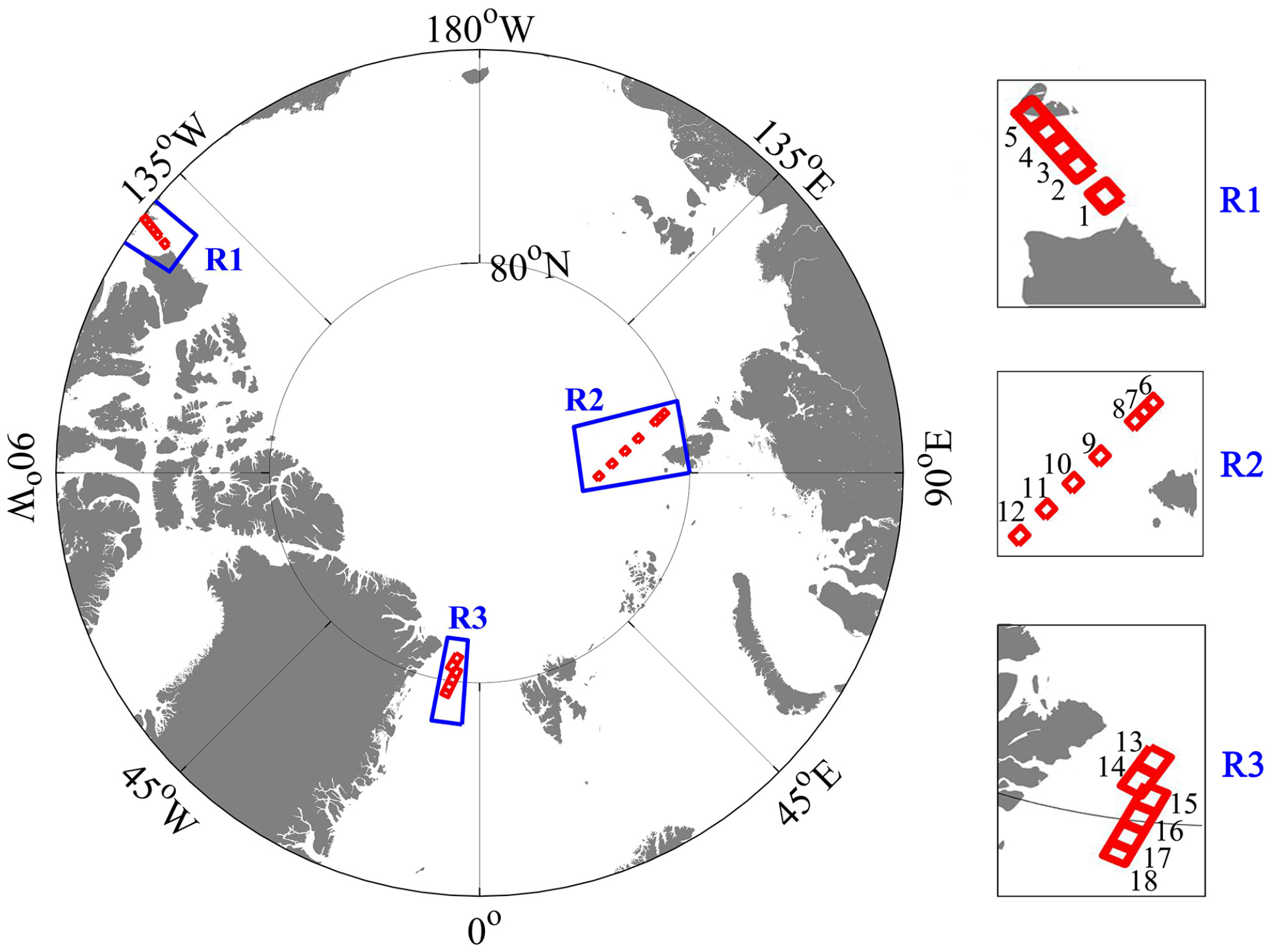
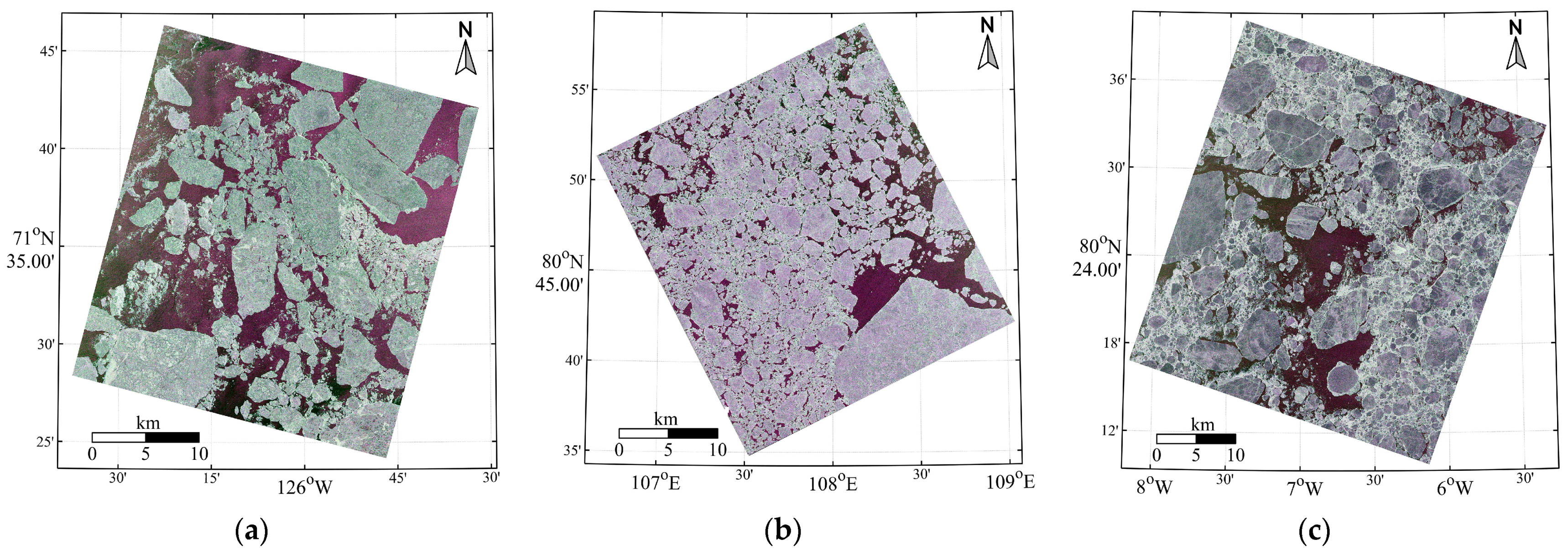
2.1. The GF-3 QPS Mode Dataset

In this study, 18 scenes of GF-3 QPS data acquired over late spring and summer Arctic sea ice were used to evaluate the sea ice classification performance based on a deep neural network approach (Section 3). Figure 1 shows the spatial distribution of these scenes in three regions. The five scenes in the Beaufort Sea, denoted as region 1 (R1), were acquired on 25 May 2017. The seven scenes located north of the Severnaya Zemlya archipelago, denoted as region 2 (R2), were acquired on 2 August 2017. The other six scenes in the Fram Strait, denoted as region 3 (R3), were acquired on 14 and 17 June 2017. According to the temperature related seasonal descriptors in [30] and the 2 m temperatures from ERA5 [31] for those three regions, the R1 and R2 scenes are in early melt season, and the R3 scenes are in advanced melt season. All the images are the Level-1A single look complex product.

Table 1. Data of the 18 scenes from GF-3.

Region	ID	Date	Acq. Time (UTC)	Swath (km)	Near inc. Angle (deg.)	Far inc. Angle (deg.)
R1	1	25 May 2017	15:11:01	18.28	35.35	37.18
	2	25 May 2017	15:11:11	18.28	35.35	37.18
	3	25 May 2017	15:11:15	18.28	35.35	37.18
	4	25 May 2017	15:11:20	18.28	35.35	37.18
	5	25 May 2017	15:11:25	18.27	35.35	37.18
R2	6	2 August 2017	09:09:01	18.10	35.39	37.20
	7	2 August 2017	09:09:06	18.13	35.39	37.20
	8	2 August 2017	09:09:11	18.15	35.39	37.20
	9	2 August 2017	09:09:30	18.24	35.38	37.20
	10	2 August 2017	09:09:44	18.30	35.37	37.20
	11	2 August 2017	09:09:59	18.34	35.37	37.20
	12	2 August 2017	09:10:14	18.32	35.36	37.19
R3	13	14 June 2017	08:01:09	24.88	37.96	40.16
	14	14 June 2017	08:01:15	24.84	37.97	40.16
	15	17 June 2017	07:37:19	27.27	41.73	43.79
	16	17 June 2017	07:37:25	27.24	41.74	43.79
	17	17 June 2017	07:37:31	27.20	41.74	43.79
	18	17 June 2017	07:37:37	27.20	41.74	43.79

summarizes the information about each scene. The imaging mode of the scenes in regions R1 and R2 was QPSI, and the imaging mode was QPSII in region R3. The nominal resolution for the R1 and R2 scenes is 8 m and for R3 it is 25 m. The incidence angle varies between 35.35° and 43.79°. All these data were acquired in conditions with a wind speed of less than 6 m/s.

2.2. SAR Data Preprocessing

The preprocessing of the GF-3 SAR data included radiometric calibration, speckle reduction, normalization, and preparation of the training data. The first three steps constitute the fundamental processing requirements when using SAR data, and normalization is a prerequisite for preparing the inputs of a deep learning method.

The GF-3 radiometric calibration method is given in the user manual as follows:

$${\mathsf{\sigma }}_{\mathrm{dB}}^0=10{\log }_{10}{\mathrm{P}}^{\mathrm{I}}\ast {\left(\mathrm{QV}/\mathrm{m}\right)}^2-{\mathrm{K}}_{\mathrm{dB}}$$

(1)

where ${\mathsf{\sigma }}_{\mathrm{dB}}^0$ is the calibrated backscatter coefficient in the unit of dB, and ${\mathrm{P}}^{\mathrm{I}}$ is the sum of the squares of the real and imaginary parts of the single look complex SAR data. The QV (qualified value) is the maximum digital value of the image before quantization and ${\mathrm{K}}_{\mathrm{dB}}$ is the calibration constant, both of which are provided in the metadata of each scene. The term m is of 32,767 for Level-1A data. Normalization of the backscattering coefficients to a fixed incidence angle for each scene was unnecessary because the variation of the incidence angle across the swath in this dataset is small, ranging from 1.8° to 2.2°.

A Lee filter was applied to reduce the speckle noise. The Lee filter accentuates the edges between ice and water with an insignificant loss of texture features. A window size of 5 × 5 pixels was used. The calibrated GF-3 SAR backscatter coefficient data was used as inputs to the adaptive Lee filter. After calibration and speckle filtering, we rescaled the backscatter coefficient dB range into a digital range of 0–255 for each region. The scaling of each region was performed for each image separately. The limits of the rescaled backscatter coefficient were set to 1.5% and 98.5% of all the polarization ranges in the given region. We then combined the different polarization data (${\mathsf{\sigma }}_{\mathrm{vv}}^0$, ${\mathsf{\sigma }}_{\mathrm{vh}}^0$, and ${\mathsf{\sigma }}_{\mathrm{hh}}^0$) into RGB format, in preparation for the input into the deep learning scheme. Figure 2 shows the color composite images of the R1-1, R2-6, and R3-15 scenes (the first two alphanumeric letters are the region designation and the third number is the ID of the scene as listed in Table 1).

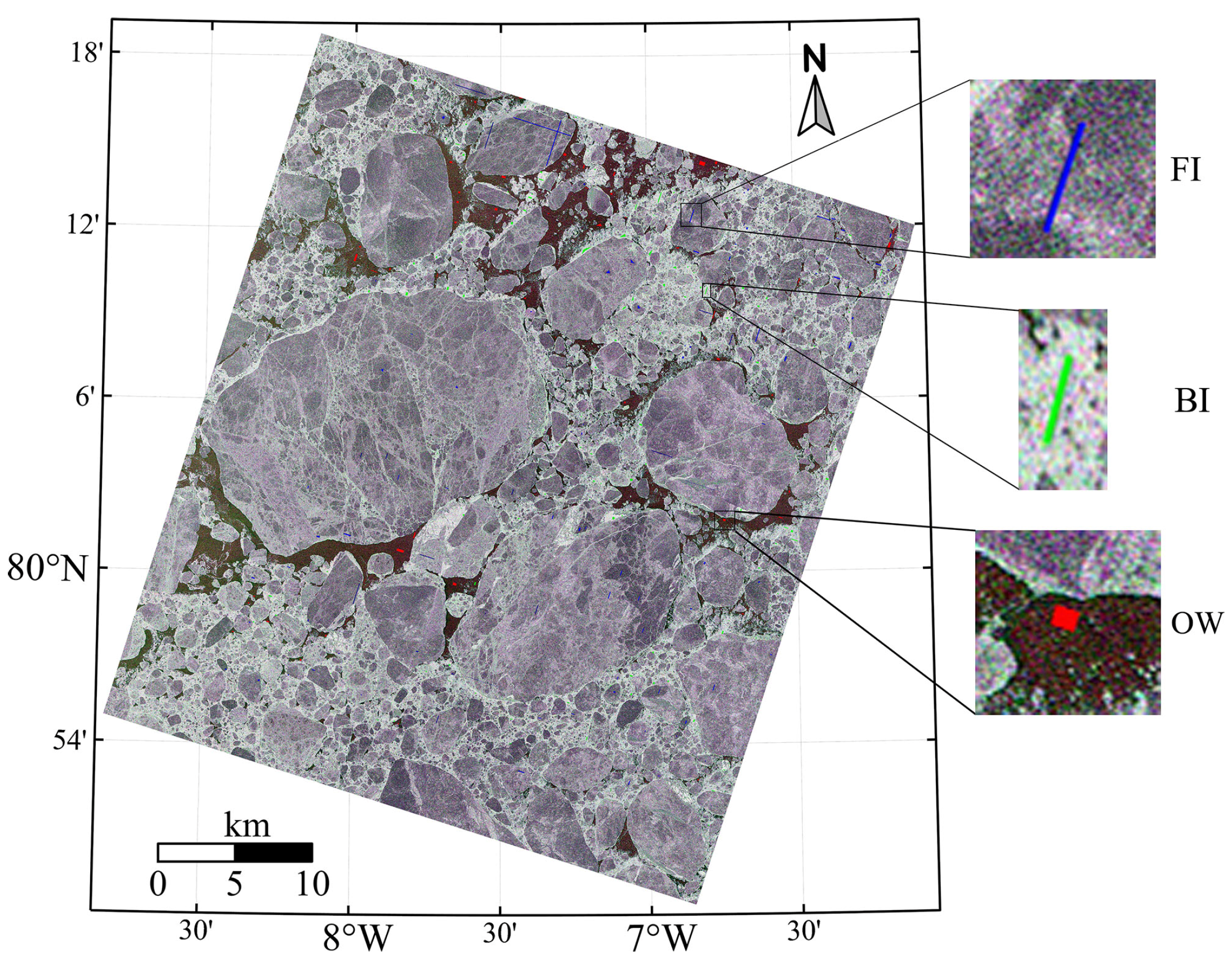
2.3. Dataset for Model Training

Ground truth data are important for implementing supervised neural network classification. The sea ice type maps released by a sea ice monitoring agency such as CIS, NIC, or AARI are commonly used as training datasets in sea ice classification studies. However, CIS ice charts are not available in all the geographic areas of the present study, and although the NIC/AARI ice charts are produced weekly, they are generated at a coarse resolution. Therefore, for the data during the melt season, the training data were generated using manual visual identification of the different sea ice types in the images.

The World Meteorological Organization (WMO) has defined seven major sea ice categories based on the ice development stage [32]. However, it is impractical to identify all these categories, especially in late spring and summer scenes when young ice types do not exist, and flooded ice surfaces can mask the underlying ice type in radar images. This results in MYI (which has a distinctly high backscatter in winter) and first-year ice (FYI) having similar radar signatures in summer. The surface deformation form, which is caused by the collision and convergence of mobile ice floes, makes the backscatter high in SAR images in both co- and cross-polarization [33]. However, the deformation may become eroded in summer or covered with wet snow, both of which reduce the backscatter. BI may also continue to exist between ice floes, and its roughness results in relatively high backscatter. Therefore, in this study, three surface categories were considered: floe ice (FI), brash ice (BI), and open water (OW). The FI category combines FYI and MYI, both of which are commonly of round or elliptical shape, with medium backscatter. The BI category represents the crushed ice between ice floes, and OW denotes the ice-free area, which has the lowest backscatter coefficient, because of its relatively smooth surface.

To construct the machine learning model (see Section 3.1), training data and validation data were required. The training data were used for developing the model. The validation data served as auxiliary data for tuning the parameters of the model to avoid overfitting and were used to improve the model capability by checking the performance of the model during the training phase.

The training and validation datasets used in developing the model were generated as follows. Firstly, we labeled the areas of the different surface types, i.e., FI, BI, and OW, in the RGB composite SAR scenes using LabelMe [34], which is an efficient open-source graphical image annotation tool. Figure 3 shows the sparse labeled areas in the composite image of the R3-16 scene, with enlarged segments representing the three surface categories of FI, BI, and OW in blue, green, and red, respectively. The labeled areas may not feature homogeneous SAR backscatter because the given surface may have a range of backscatter. The labeled areas were randomly selected but evenly distributed within the image space, and they occupy a small percentage (about 0.14%) of the entire image area.

For each pixel in the labeled area of each type, the pixel and its neighboring pixels in the composite SAR image were extracted as a patch. Each patch was considered to represent a single surface type, i.e., the type of the center pixel. Figure 4 depicts a virtual segment in an image, with the three colors representing the three surfaces of FI, BI, and OW. For instance, the black outer boundary represents the labeled area, with all the pixels inside representing the FI surface. For each pixel within the labeled area, a window is established. This is shown in the dotted lines for pixels “a”, “b”, “c”, and “d”. The window is 3 × 3 pixels in this example, where the window constitutes one patch. With the changing of the window size, the surface type information contained in a given patch becomes different. To determine the most appropriate information content for GF-3 QPS mode data for the algorithm, four patch sizes were tested in this study, i.e., 25 × 25, 31 × 31, 37 × 37, and 43 × 43. All the pixels within a patch constituted a training sample, which was used as the input for the deep learning network. As a patch may contain peripheral pixels, the surface types of the pixels within the same patch can be different. As the VV, VH, and HH polarizations were considered, each image patch was a 3-D matrix of size, 31 × 31 × 3. The number of generated patches is equal to the number of pixels in all the labeled area. Of the generated patches, 80% were randomly selected as training data, and the other 20% were used for the validation. We did not reject any training data. The number of training samples for the R1, R2, and R3 scenes were 207,409, 219,888, and 344,043, respectively, and the ratios of FI, BI, and OW were about the same in each scene.

The composite images of the R1-1, R2-6, and R3-15 SAR scenes were used to test the performance of the final trained model for each region, respectively, and the rest of the scenes in each region were used for the labeling and making the training data. The training scenes were not used for the testing, considering the possible overfitting of the machine learning.

3. Methodology

In this study we constructed a deep neural network structure called MSI-ResNet for classifying the three surface types of FI, BI, and OW in the GF-3 SAR QPS data. This structure is based on ResNet V2 [19] after shrinking and modifying the original network to allow for classification of a small number of categories in high resolution SAR imagery as the input data. In the field of machine learning, different patch sizes and inputs will have an influence on the classification results. Based on MSI-ResNet, the effect of the patch size and the classification performance of different polarization combinations of GF-3 QPS mode data were explored. For the classification result assessment, a stratified random sampling method was used to compare the results with the visual classification of the surface types in the SAR images. To further assess the MSI-ResNet classification results, the results were also compared with the classification results obtained using the SVM classifier. The specifics of the MSI-ResNet structure and stratified random sampling method are respectively presented in Section 3.1 and Section 3.2. Data from the images with an ID of 1, 6, and 15 (Figure 1 and Table 1) were selected for performing the accuracy evaluation for each region, and the other data in the same region were used for the training.

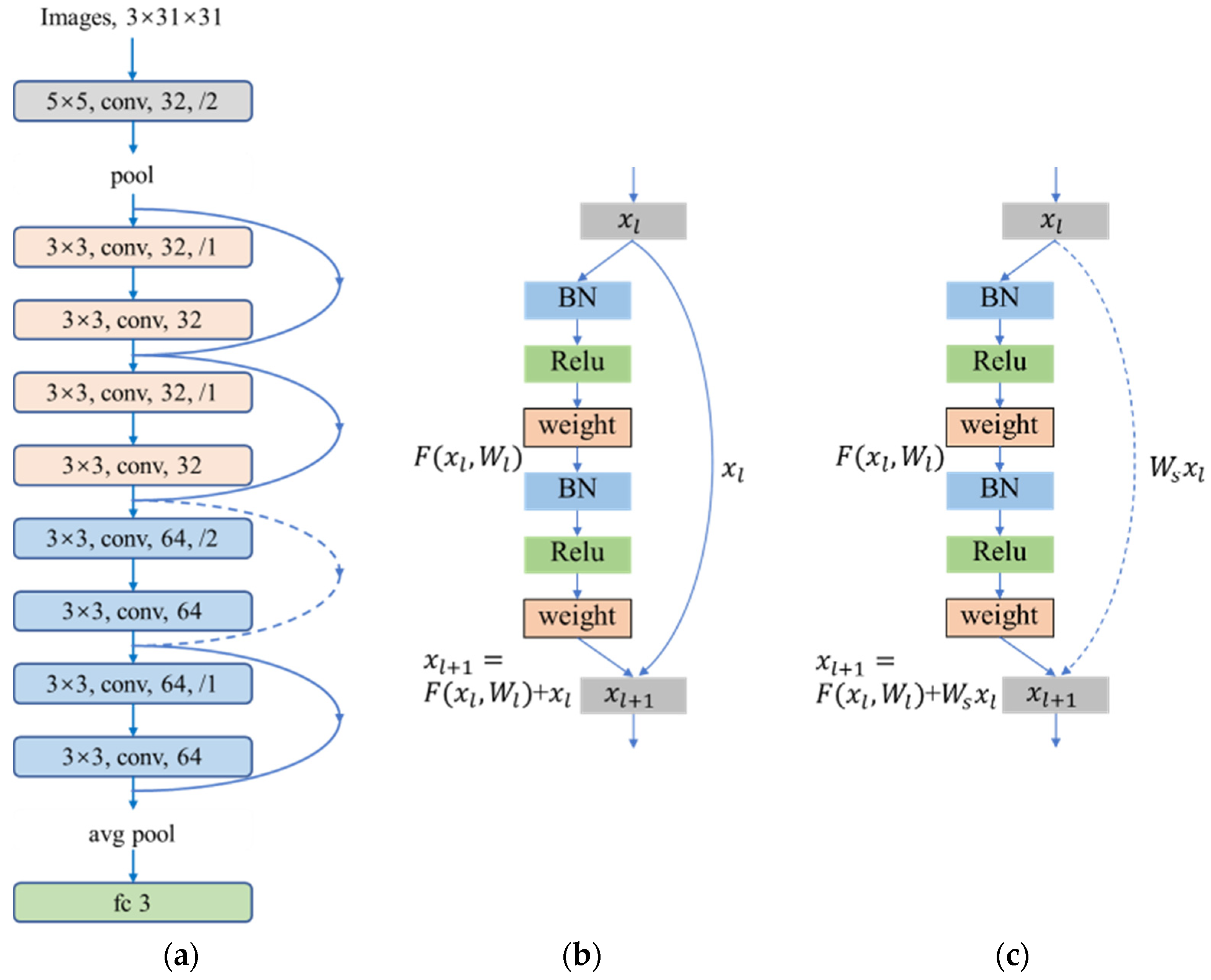
3.1. Structure of MSI-ResNet

A neural network is able to establish the intrinsic connection between input–target pairs when they are well associated [35]. A deep learning network, which is also known as a deep neural network, consists of an input layer, hidden layers, and an output layer. The hidden layers include convolutional layers, pooling layers, and fully connected layers. A convolutional layer (conv) functions as a feature extractor by convolving with the input data, generally using multiple kernels of a specific size. The convolved features are then nonlinearized by an activation layer to produce the feature maps. A pooling layer compresses the feature map to reduce its redundancy and converts the output to a vector during the last pooling process. All the learned features of the previous layers are combined by the fully connected (fc) layer to determine the desired patterns.

Deep learning models have been widely used in image classification. Among the different models, deep residual neural network models, and especially the ResNet V2 model, can solve the problem of gradient explosion and gradient disappearance. Therefore, according to the characteristics of SAR remote sensing imagery and the principle of the ResNet V2 model, we designed a lightweight deep residual neural network model for sea ice classification, i.e., MSI-ResNet, based on pixels (Figure 5a). The model effectively shortens the training time, while improving the training efficiency and classification accuracy.

The MSI-ResNet model is structured in 10 layers, as shown in Figure 5a, with input images of a size of 3 × 31 × 31. The first convolutional layer’s kernel size is 5 × 5, the stride is 2, and the number of convolution kernels is 32. It is the largest layer of convolution kernels in the model to obtain the features of large neighborhood of the model and image denoising. The resulting vectors are processed using max pooling with a stride of 1. Four residual blocks follow, each of which consists of two convolutional layers with the kernel size of 3 × 3, and the inputs of each block are connected with the outputs using an arrowed curve. The kernel number generally increases as the neural network becomes deeper to learn more features of the specific inputs. Each convolutional layer in the first two residual blocks has 32 kernels, and there are 64 kernels for the last two blocks in the structure of MSI-ResNet. The stride of the third block changes to 2 in order to decompress the outputs of that block as the channel number doubles, while all the other blocks remain with a default stride of 1. This leads to dimension inconsistency in the third residual block, whose input and output dimensions are 64 × 14 × 14 and 64 × 7 × 7, respectively. We use the dotted curve to represent this in Figure 5a. The other three solid lines refer to a consistent dimension connection for the blocks. The specific structure of these two residual blocks are shown in Figure 5b,c, respectively. After the residual blocks, the image is processed by average pooling to reduce the dimension of the image, and a vector of 64 × 1 × 1 is obtained, which greatly reduces the computational load. The last layer is a fully connected layer, which outputs the probability of the center pixel of the input image belongings to each kind of surface type.

As mentioned above, there are two types of blocks in the MSI-ResNet model, as shown in Figure 5b,c. Each block consists of three layers: a batch normalization (BN) layer, a rectified linear unit (ReLU) activation layer, and a weight layer (the parameters of that convolution). In addition to the residual block itself, the BN is carried out to prevent the gradient from disappearing and exploding in each residual block, which can effectively improve the training efficiency. Suppose that the input of the $l$-th residual block is $x_l$ and the output is $x_{l+1}$. In most cases (as shown in Figure 5b), in a residual block $x_l$ performs two convolution operations $W_l$ with the step size of 1. The residual $F\left(x_l,W_l\right)$ plus $x_l$ gives $x_{l+1}$:

$$x_{l+1}=F\left(x_l,W_l\right)+x_l$$

(2)

The dimensions of $x_l$ and $F$ must be equal in Equation (2) to conduct the addition operation. In another case (Figure 5c), as shown in the third residual block in Figure 5a, the number of channels and the size of each channel have changed which will cause the inputs and outputs to have different dimensions as mentioned above. To achieve the addition operation for $x_l$ and $F\left(x_l,W_l\right)$, a convolution operator $W_s$ is needed for $x_l$ to make the convolved $W_s{x}_l$ and $F\left(x_l,W_l\right)$ have the same channel number and size. The calculation formula is:

$$x_{l+1}=F\left(x_l,W_l\right)+W_s{x}_l$$

(3)

We set the learning rate to 0.0001, the weight decay to 0.0001, the BN decay to 0.997, and the batch norm scale to 10⁻⁵. The classifier is the SoftMax function.

The loss function is the SoftMax-cross-entropy cost function, which is defined as:

$$loss = -\frac{1}{n}{\displaystyle \sum }_{i=1}^n\left[y_i\ln h\left(x_i\right)+\left(1-y_i\right)\ln \left(1-h\left(x_i\right)\right)\right]$$

(4)

where $h\left(x_i\right)$ is the predicted output, $y_i$ is the expected output, $n$ is the total number of samples, and $x_i$ is an input vector.

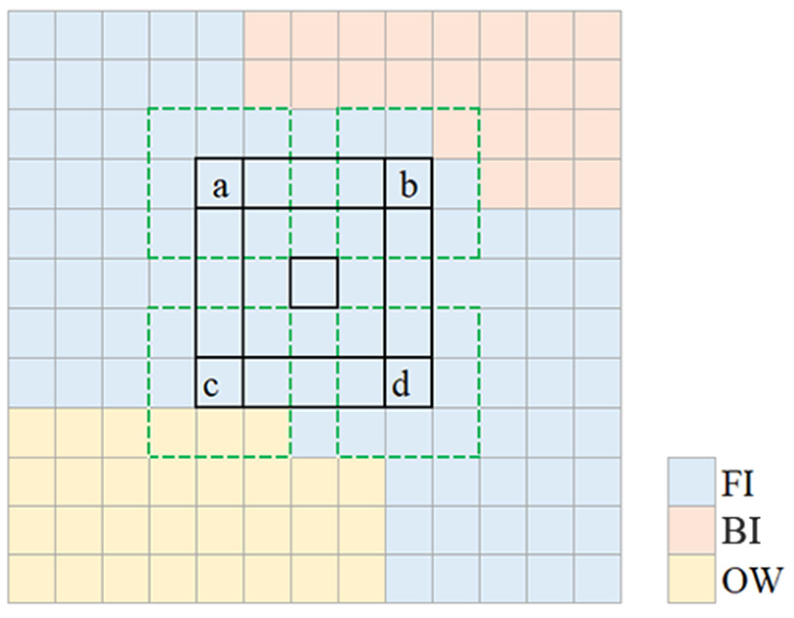
3.2. The Stratified Random Sampling Assessment Method

Due to the large width and resolution of SAR image coverage, it is always difficult to obtain accurate reference data by field measurement or manual annotation. Evaluation of the classification accuracy is thus usually conducted by the use of sampling and constructing an error matrix. Stratification is a common technique for data sampling when there are certain subdivisions in the imagery. If a random sample is taken in each stratum, the whole procedure is described as stratified random sampling which guaranteed that the strata have already been constructed. The stratified random sampling method allows each stratum to have different classification accuracy expectations [36]. As a result, stratified random sampling has been applied to many remote sensing image classification accuracy assessment tasks [37,38]. One of the convenient forms of stratified random sampling formulas for any allocation with continuous data is given as follows [36]:

$$n= \frac{{\left(\sum W_h{S}_h\right)}^2}{V+\left(1/N\right)\sum W_h{S}_h^2}$$

(5)

where the term $n$ is the number of samplings for each stratum, the suffix $h$ denotes the stratum, $W_h= N_h/N$ is the stratum weight, $N_h$ is the total number of units, $N$ is the total number of units. In our study, $N$ is the total pixel number of the validation image. $S_h^2$ is the unbiased estimate of the true variance for a certain stratum (the divisor for the variance is $N_h$−1). $S_h^2= U_h\left(1-U_h\right)$, where $U_h$ is the expected user’s accuracy for each stratum. We set the user’s accuracy values of FI, BI, and OW as 0.7, 0.9, and 0.95, respectively, which are appropriate values, according to the previous research [10,16,39]. The term $V$ is the desired variance of all the estimates, which was specified as 0.01 in this study.

4. Results and Assessments

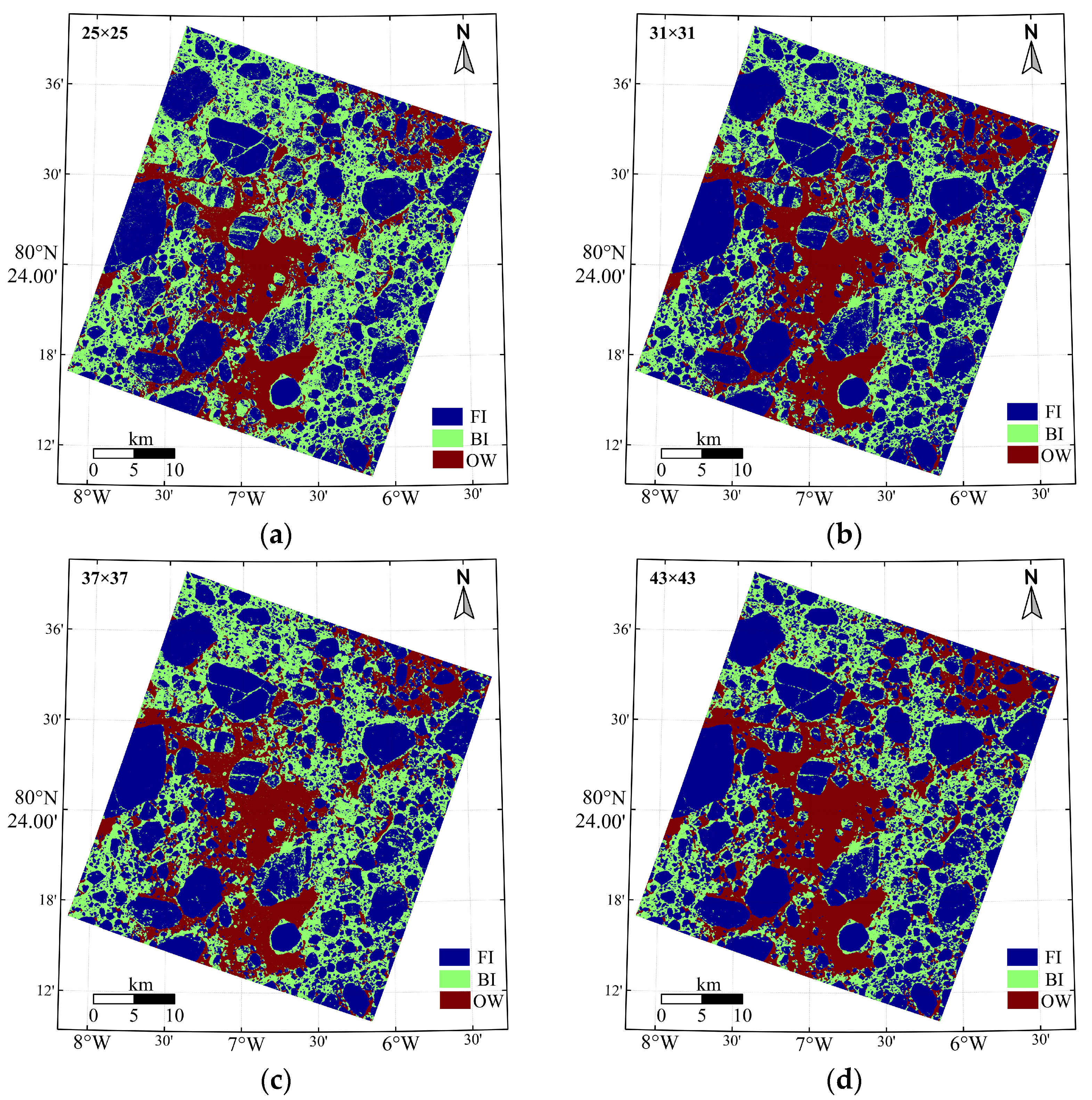
4.1. Experiments with the Patch Size

Figure 6 depicts the results of the sea ice classification of the R3-15 scene using patch sizes from 25 to 43 with a step size of 6 using the MSI-ResNet method with the VV, VH, and HH polarization combination as input. The blue, green, and red colors denote FI, BI, and OW, respectively. The assessment of the classification accuracy was performed based on visual interpretation of the imagery. Random sampling from each ice type was used while maintaining the proportion of the samples from each class. The confusion matrix is shown in

Table 2. Sea ice classification confusion matrix for the R3-15 scene data based on MSI-ResNet with patch sizes of 25 × 25, 31 × 31, 37 × 37, and 43 × 43.

Patch Size	Ice Type	FI	BI	OW	User’s Accuracy (%)	Producer’s Accuracy (%)	Overall Accuracy (%)	Kappa	Fraction (%)
25 × 25	FI	565	19	6	95.76	90.98	90.53	0.85	46.18
	BI	53	379	16	84.60	89.81			35.02
	OW	3	24	213	88.75	90.64			18.80
31 × 31	FI	687	21	9	95.12	96.33	94.67	0.91	53.04
	BI	21	341	3	93.42	90.21			27.04
	OW	3	10	256	95.17	96.60			19.92
37 × 37	FI	473	25	1	94.79	91.67	90.10	0.85	48.98
	BI	39	267	7	85.30	80.42			29.80
	OW	4	40	316	87.78	97.53			21.22
43 × 43	FI	639	26	2	95.80	93.70	89.53	0.83	51.02
	BI	36	296	5	87.83	77.28			25.74
	OW	7	61	231	77.63	97.12			23.24

.

The user’s accuracy is the correctly classified pixels in a category divided by the total number of pixels that are classified into that category. The producer’s accuracy is the number of the correctly classified pixels of a category divided by the number of reference pixels selected from the training data [40,41]. The overall accuracy combines these two measures. The kappa coefficient takes the bias caused by sample size differences into account, so that it can be used to evaluate the consistency between the model prediction results and the actual classification results. A high kappa coefficient value means high consistency. Table 2 shows that the overall accuracy and kappa coefficient reach their maximum values (94.67% and 0.91, respectively) when the patch size is 31 × 31, and their minimum values (89.53% and 0.83, respectively) when the patch size is 43 × 43. This means that the patch size may add noise that hinders the development of the machine learning, and hence affects the classification accuracy. We recommend exploring the optimal patch size to refine the accuracy of the classification.

Considering all the examined patch sizes, the average user’s (producer’s) accuracies for FI, BI, and OW are 95.37% (93.17%), 87.79% (84.43%), and 87.33% (95.47%), respectively. When using the minimum and maximum patch sizes in Table 2, the variation range of the user’s (producer’s) accuracy is 1.01% (5.35%), 8.83% (12.93%), and 17.54% (6.89%) for FI, BI, and OW, respectively, and the corresponding variance is 0.25 (5.76), 16.04 (43.17), and 52.57 (10.53), respectively. The FI shows the highest classification accuracy, which remains relatively steady with the changing patch size. The accuracy of BI is more variable than that of FI, with the largest variance of the producer’s accuracy. The OW is most sensitive to the patch size, and shows the highest accuracy variance.

The patch size of 31 × 31 was used in the subsequent exploration. The OW is overestimated in all the patch sizes since its user’s accuracy is always lower than the producer’s accuracy. As for the resulting fractions of these three ice surfaces (Table 2), the OW fraction increases from 18.8% to 23.24% as the patch size increases, which is very different to the fluctuations for FI and BI.

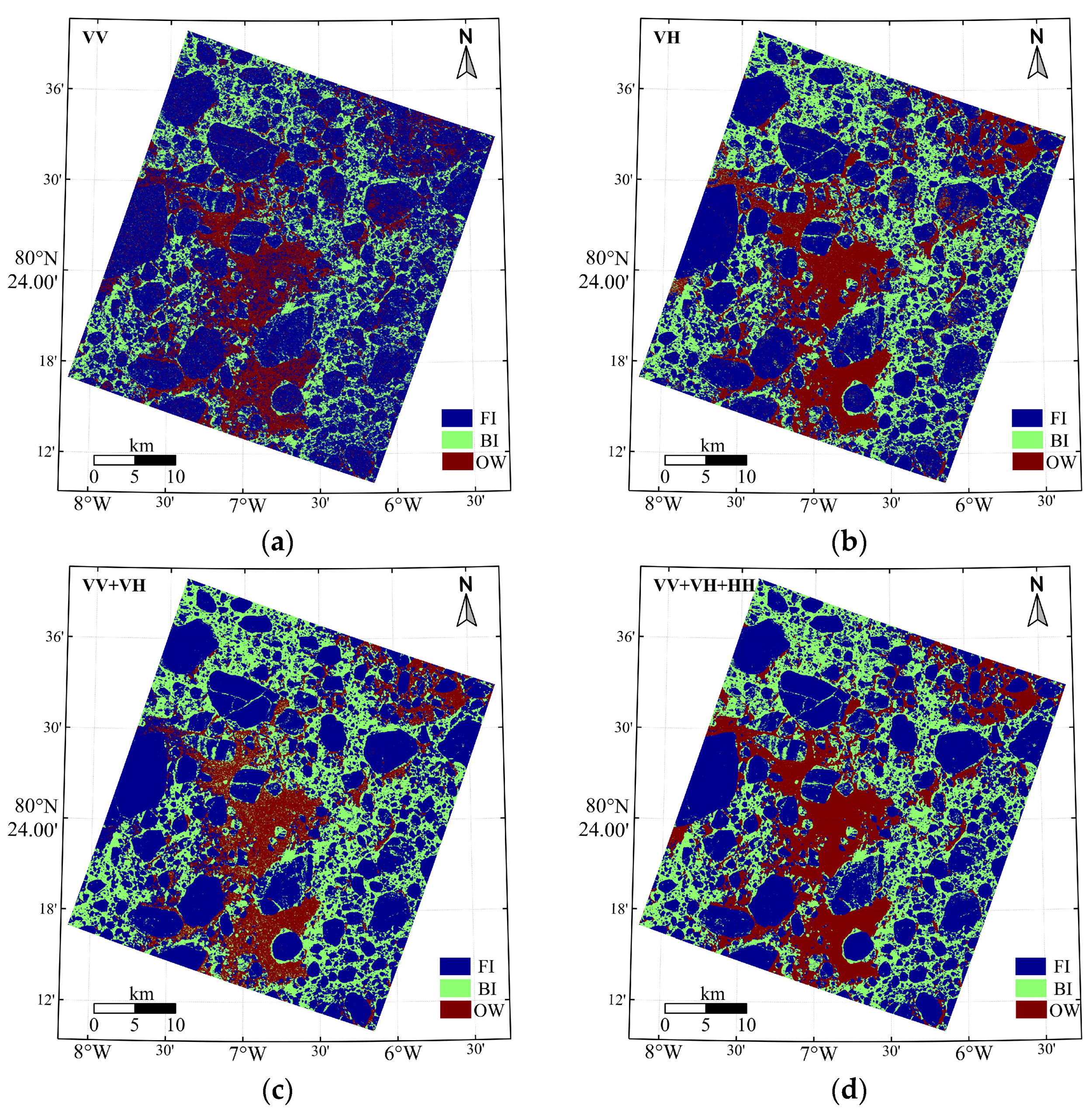
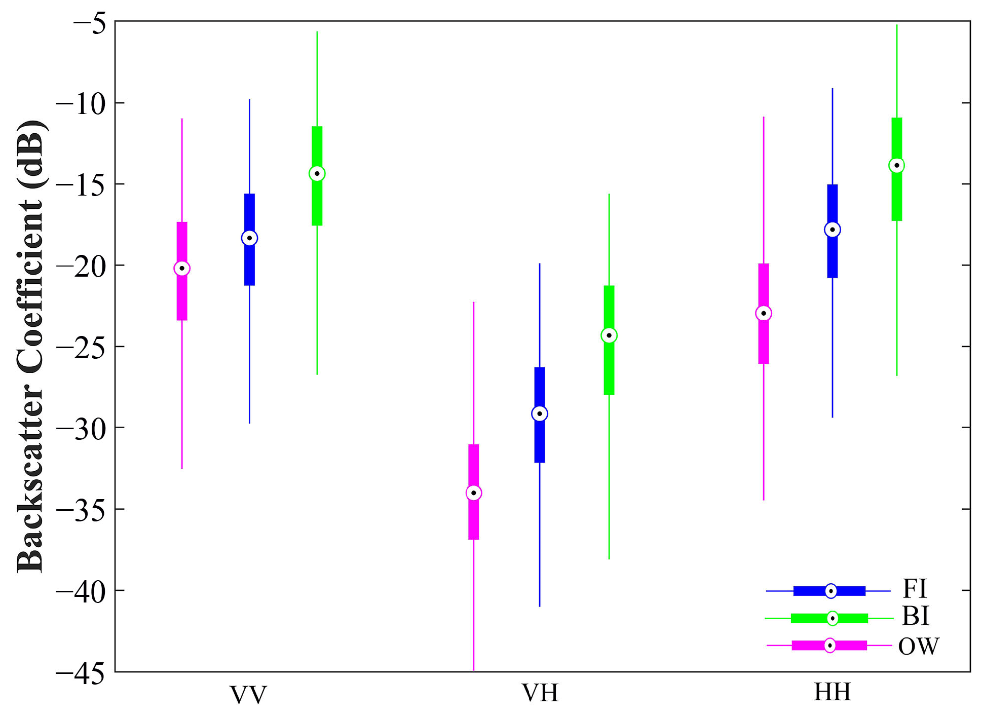
4.2. Experiments with Polarization Data Combination

The classification results for the R3-15 scene obtained by MSI-ResNet with different polarization combinations and a patch size of 31 × 31 are presented in Figure 7, and the corresponding confusion matrix is shown in

Table 3. Sea ice classification confusion matrix for the GF-3 QPS R3-15 mode data based on MSI-ResNet with different polarization combinations.

Patch Size	Ice Type	FI	BI	OW	User’s Accuracy (%)	Producer’s Accuracy (%)	Overall Accuracy (%)	Kappa	Fraction (%)
VV	FI	786	129	54	81.11	93.46	83.37	0.70	54.27
	BI	10	282	6	94.63	67.46			26.36
	OW	45	7	190	78.51	76.00			19.38
VH	FI	689	30	24	92.73	92.98	91.09	0.85	64.20
	BI	31	323	7	89.47	89.23			19.75
	OW	21	9	235	88.68	88.35			16.05
VV + VH	FI	833	57	36	89.96	97.54	91.12	0.85	62.40
	BI	17	292	4	93.29	78.28			21.07
	OW	4	24	332	92.22	89.25			16.53
VV + VH + HH	FI	687	21	9	95.12	96.33	94.67	0.91	53.04
	BI	21	341	3	93.42	90.21			27.04
	OW	3	10	256	95.17	96.60			19.92

. Noticeably, Figure 7d is the same as Figure 6c. In these experiments, only one type of copolarization data (VV polarization) was used. Additionally, as the VH and HV polarizations are physically reciprocal, only the VH cross-polarization was considered.

Table 3 shows that the overall accuracy and kappa coefficient increase with the added polarization data. The combination of the three polarizations results in the maximum accuracy and kappa coefficient. The improvement over using VV only, VH only, and the combination of VV + VH is 11.3%, 3.58%, and 3.55%, respectively. The worst discrimination result is with the single VV polarization as the input data. The VH polarization leads to a similar overall accuracy and kappa to that obtained from using the combination of VV and VH polarization inputs, at around 91% and 0.85, respectively. This is an improvement of about 7.7% and 0.15 (respectively) compared to the use of VV polarization only.

The average user’s (producer’s) accuracy for FI, BI, and OW is 89.51% (94.77%), 91.83% (81.13%), and 88.65% (87.55%), respectively, when considering the VV, VH, VV + VH, and VV + VH + HH polarization combinations together. This also shows the approximate order of the feasibility of the identification of each surface.

Using the single VV polarization, the classification of the BI surface type achieves the highest user’s accuracy of 94.63% and the lowest producer’s accuracy of 67.46%. Most of the BI is misclassified into the overestimated FI, as shown in Figure 7a and Table 3. The VH polarization experiment results in similar user’s and producer’s accuracies for every ice type, as well as OW. The overall accuracy from using the copolarization VV data is higher, especially for FI and OW discrimination. In short, when dual-polarization or multipolarization data are used for sea ice classification, the proportion of FI misclassification is greatly reduced, which also improves the classification accuracy of BI and OW.

Almost all the ice types achieve the maximum user’s and producer’s accuracies with the three polarizations as input data, except for the producer’s accuracy of BI, which shows the highest value using the VV and VH polarization combination. Furthermore, all the ice types show the minimum accuracy when using the copolarization input. The classification accuracy for the VV and VH polarization combination is slightly higher than that when using VH polarization only, but is very much better than the results obtained when using the VV polarization. This confirms that using dual- or quad-polarization data can improve the sea ice classification precision when compared to using single polarization data. The improvements in the overall accuracy and kappa from dual to quad modes are 3.55% and 0.06, respectively.

Figure 8 shows the box-whisker plots of the backscatter coefficient statistics of the three surface types from all the images in the R3 region based on the sea ice classification results obtained using the MSI-ResNet method with the input of the VV, VH, and HH polarization combination and a patch size of 31 × 31. The circles denote the median values. The values corresponding to the upper and lower boundaries of each solid rectangle are the upper quartile (Q3) and lower quartile (Q1), respectively, and Q3−Q1 is the interquartile range (IQR). The upper and lower extremes of each box-whisker plot are the Q3 + 1.5*IQR and Q3 − 1.5*IQR, respectively. The lower limits of the box-whisker plots in Figure 8 suggest that the noise equivalent sigma zero (NESZ) values of the VV, VH, and HH polarizations are approximately −33, −45, and −33 dB (near to the 40–42° incidence angle), which are comparable values to those reported in previous GF-3 research [23,24]. The median backscatter coefficient values of FI, BI, and OW in the VV polarization in Figure 8 are closer together than in the VH polarization, which confirms that the classification performance of the VH polarization is better than that of the VV polarization. The separation between the three types in the HH polarization is better than that in the VV polarization, which results in the overall accuracy being further improved when the three polarizations are used together.

4.3. Application and Comparison

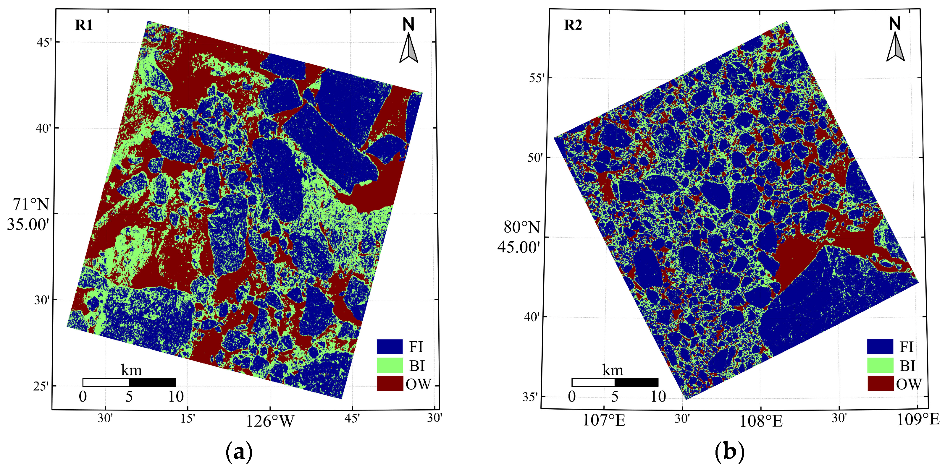
4.3.1. Classification of the R1-1 and R2-6 Scene Images

To further investigate the stability of the sea ice classification performance of GF-3, another two sea ice classification experiments based on MSI-ResNet were conducted using the R1-1 and R2-6 scene data. The related results are shown in Figure 9 and

Table 4. Sea ice classification confusion matrices for the R1-1 and R2-6 scene data based on MSI-ResNet, and the R3-15 scene data based on the LibSVM classifier.

Data (Classifier)	Ice Type	FI	BI	OW	User’s Accuracy (%)	Producer’s Accuracy (%)	Overall Accuracy (%)	Kappa
R1-1 (MSI-ResNet)	FI	480	9	10	96.19	97.76	94.62	0.92
	BI	11	269	33	85.94	96.76
	OW	0	0	360	100.00	89.33
R2-6 (MSI-ResNet)	FI	838	38	9	94.69	98.70	94.23	0.90
	BI	11	283	22	89.56	87.08
	OW	0	4	251	98.43	89.00
R3-15 (LibSVM)	FI	746	57	36	88.92	92.21	89.04	0.81
	BI	38	308	1	88.76	84.38
	OW	25	0	222	89.88	85.71

. For each experiment, the VV, VH, and HH polarization combination data were used with a patch size of 31 × 31.

The R1-1 images of the Beaufort Sea in late spring (Figure 2) contain many scattered large ice floes with rough surface, scattered ice debris, brash ice, and extended open water with a visible wave induced rough surface in the northwest part of the scene. On the other hand, the R2-6 image (north of the Severnaya Zemlya archipelago in midsummer) contains many small ice floes surrounded with crushed ice. The overall accuracies (kappa) for those two areas are 94.62% (0.92) and 94.23% (0.90), respectively, which are as high as the results for R3-15 when using MSI-ResNet (in Table 2). For each region, the FI shows the best classification results from the aspect of both the user’s and producer’s accuracies. The user’s accuracy for OW is much higher than the producer’s accuracy in these two cases, unlike the case for the R3-15 scene, which indicates that the OW is slightly underestimated. Moreover, the BI is overestimated in the R1-1 scene, with a relatively low user’s accuracy.

4.3.2. Comparison with the SVM Classifier

The results of the classification of the R3-15 (Table 3) scene obtained using MSI-ResNet are compared to the results achieved using the LibSVM classifier [29] in Table 4, where calibrated, filtered, and scaled VV, VH, and HH backscattering coefficients were used. The related parameters for LibSVM used in this study were 8, 17, and 31 × 31 for the displacement, quantization, and region size, respectively, based on former studies of the sea ice classification of SAR data [42]. The radial basis function was chosen as the kernel for the application of LibSVM. The training data were 4000 FI pixels, 4000 BI pixels, and 4000 OW pixels. The classification results are displayed in Figure 10 and Table 4. The results of the LibSVM classifier show an overall accuracy and kappa coefficient of 5.63% and 0.1, respectively, which are both lower values than the results obtained from using MSI-RestNet. In addition, the FI is overestimated when using the LibSVM method. Improving the accuracy of FI detection may be the main direction of future optimization when using this method by testing the sensitivity of the displacement, quantitative, region size, and number of training samples.

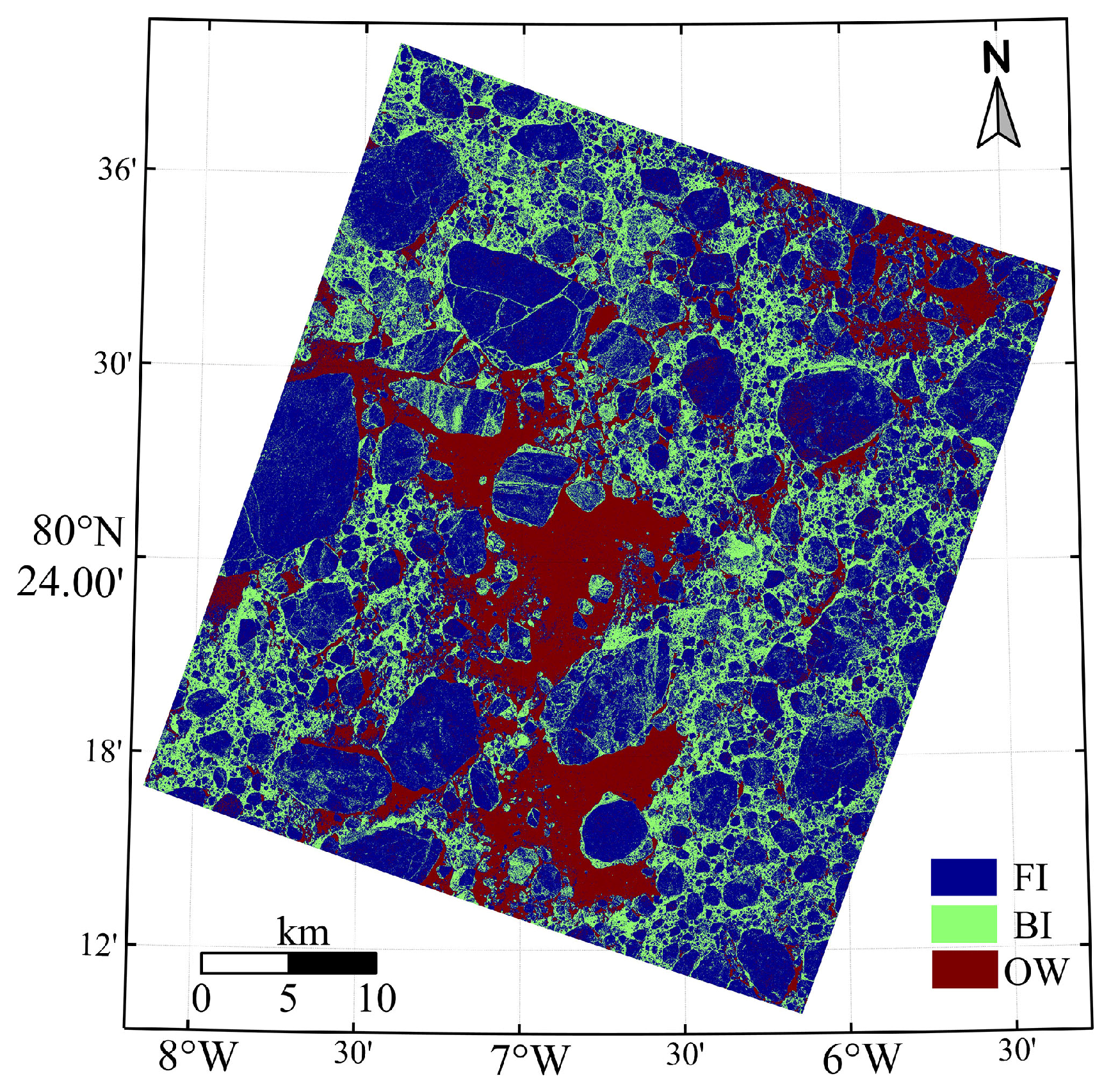
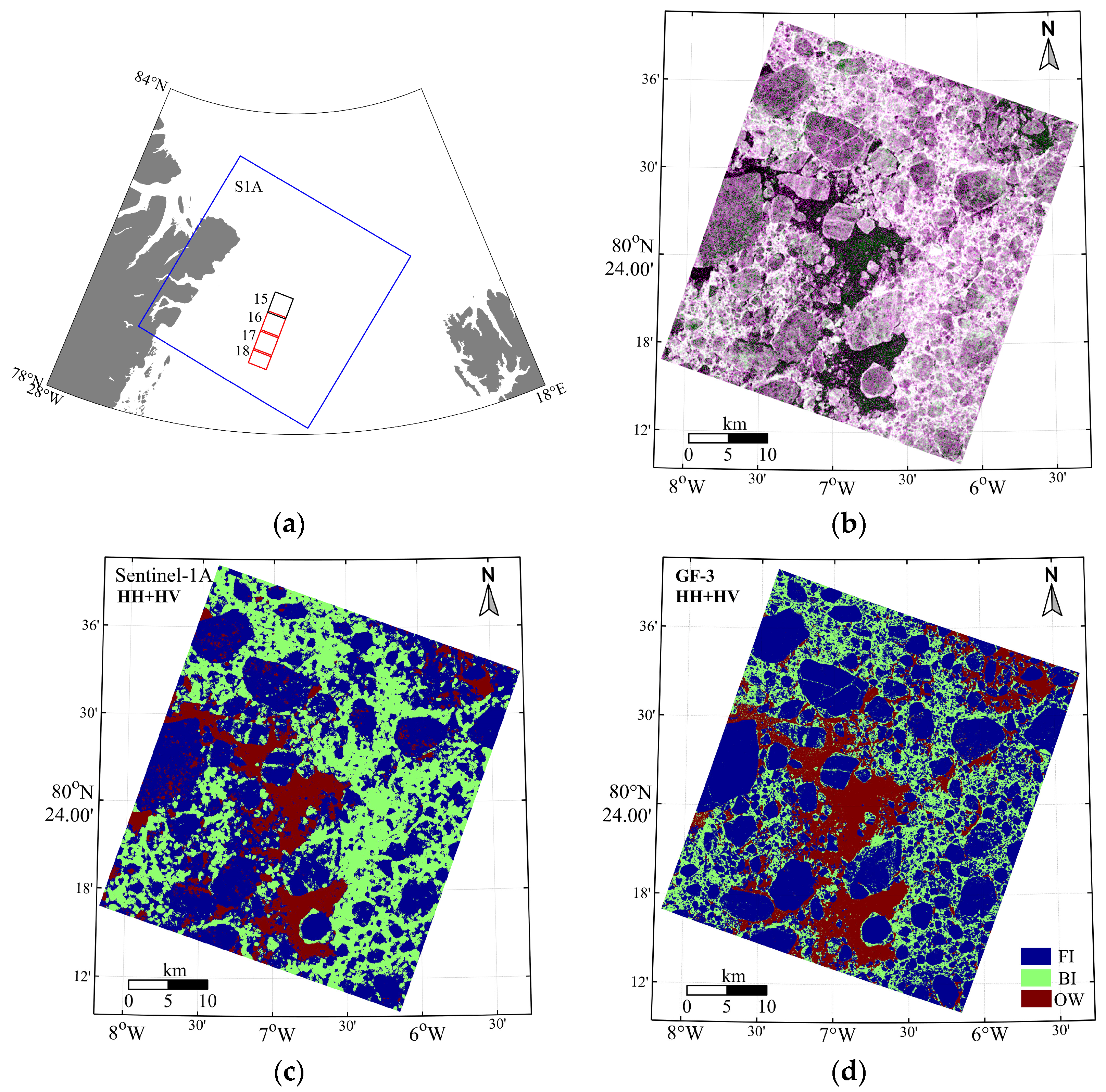
4.3.3. Comparison with Sentinel-1 SAR Classification

For a comparison with the data of another SAR sensor, and to explore the applicability of the MSI-ResNet method, a scene of near-coincident Sentinel-1A (S1A) EW swath mode data, covering the GF-3 R3-15 to R3-18 scenes was processed using the MSI-ResNet classifier. The S1A scene was acquired on 17 June 2017 at 08:17 UTC, which was 41 min later than the GF-3 scene acquisition. The nominal cover is 400 × 400 km and the pixel spacing is 40 × 40 m. The EW mode at a slightly higher spatial resolution than the GF-3 QPS mode data was adopted for the comparison as it is the only mode of S1A that covers the 18 scenes of GF-3 data used in this study. The S1A Interferometric Wide mode data with a higher resolution of 10 m are unavailable in the coverage of our research region. Figure 11a shows the geographic location and coverage of the S1A scene (with the blue rectangular box). The coincident coverage of S1A over the area of the R3-15 scene (the black box in Figure 11a) was classified using the MSI-ResNet classifier, while the coincident coverages of scenes R3-16, R3-17, and R3-18 (the red box in Figure 11a) were used for the training.

The S1A false-color image for scene R3-15 is shown in Figure 11b. Regardless of the differences in the number of polarization channels and pixel spacing, the composite images of both GF-3 and S1A in the same area of R3-15 are visually very similar. All the polarization (HH and HV) images of S1A were radiometrically calibrated, Lee filtered, and scaled before the training. The improved and effective denoising method proposed in [43] was applied for the elimination of the additive and residual noise of the HV polarization. The variation of the incidence angle across the extracted subimage of S1A was small and therefore ignored. The patch size of 7 × 7 was found to have a better accuracy than 15 × 15 or 31 × 31 (not provided in the text), and was adopted for the S1A classification experiment. The accuracy assessment method of stratified random sampling was also applied for the S1A data.

The classification image from S1A in Figure 11c is compared to the classification data from GF-3 R3-15 in Figure 11d which is the result of GF-3 with dual-polarization data (HH and HV) as the input in the MSI-ResNet classifier. Qualitatively speaking, the results are similar. The quantitative classification confusion matrix is presented in

Table 5. Sea ice classification confusion matrix for the Sentinel-1A scene of the R3-15 scene and the GF-3 R3-15 scene based on MSI-ResNet.

Data (Method)	Ice Type	FI	BI	OW	User’s Accuracy (%)	Producer’s Accuracy (%)	Overall Accuracy (%)	Kappa
Sentinel-1A (HH + HV)	FI	658	54	26	89.16	89.52	88.03	0.79
	BI	64	411	1	86.34	87.26
	OW	13	6	137	87.82	83.54
GF-3 (HH + HV)	FI	750	54	10	92.14	96.53	92.08	0.84
	BI	25	312	4	91.50	81.46
	OW	2	17	240	92.66	94.49

. The application of MSI-ResNet to the S1A data results in good discrimination of large ice floes and OW, with a user’s accuracy of 89.16%, and 87.82%, respectively, which is comparable with the GF-3 results obtained using dual-polarization inputs, as shown in Figure 11d. Nevertheless, this approach is weaker in identifying the scattered tiny ice floes surrounded by BI, when compared with Figure 11d, which causes the overestimation of BI. This can be attributed to either the similar backscatter coefficients in the sea ice mixed region, the training data labeling or the patch size selection. In general, the GF-3 QPS mode data can capture more specific details in the discrimination of sea ice classification, especially for the scattered ice floes, than the S1A EW mode data with the MSI-ResNet method.

5. Discussion

In this study, we used 18 scenes acquired by the polarimetric SAR sensor onboard the Chinese GF-3 satellite to classify sea ice in late spring and summer in the Arctic Ocean, with the assumption that all the scenes have the same surface cover types, namely, floe ice, brash ice, and open water. The warm weather in summer induces flooding or snow melting of the ice floe surfaces, which lowers the backscatter of the ice floe surfaces. It also causes the melting of thin FYI and thus the expansion of the open water area, which increases the mobility of the ice floes and leads to formation of more brash ice. The study was limited in data and space, using only the 18 available scenes acquired over four days from three regions. The wind speed during the data collection did not exceed 6 m/s, and the incidence angle range across the 30-km swath of each scene was less than 3°. We believe that this study is the first attempt to investigate the performance of GF-3 data in sea ice classification. Therefore, in this paper, it was necessary to provide comparisons with the other sensors used in previous studies.

Areas of low backscatter intensity, such as the flooded or snow melting surfaces of sea ice, are usually contaminated by system noise. The NESZ is a measure of the sensitivity of a given SAR system to areas of low backscatter [44]. Low backscatter areas, especially under low wind, large incidence angle, and cross-polarization conditions, can be well observed by SAR systems, with low NESZ values [45]. The empirically estimated NESZ values for GF-3 QPS mode shown in Figure 8 (under a wind speed of <6 m/s and an incidence angle of about 40°) are very low, and are comparable with the NESZ values of other C-band SAR sensors at the same incidence angle, e.g., −33 dB (HH, VV) and −34 dB (HV, VH) for Radarsat-2 fine quad mode data [46] and lower than the −22 dB for S1A EW mode data [45,47]. Notably, the low NESZ achieved by the cross-polarization denotes the good observation capabilities of GF-3 quad-polarization data in polar sea ice monitoring.

The backscatter coefficient is an essential parameter for surface classification in SAR images. It is triggered by different scattering mechanisms [48], and is affected by the surface properties, sensor parameters, and viewing geometry. Backscatter in measured in terms of its intensity, phase, and polarization. The polarization is particularly important when discriminating ice from the surrounding open water. This is because the ice surface may depolarize the backscatter if the surface becomes deformed or very rough, while the water surface does not depolarize the backscatter, no matter how wind-roughened the surface is [33]. The cross-polarization observations have been recognized as a good tool to discriminate sea ice from open water [49,50,51]. The reduced sensitivity to changes in incidence angle makes cross-polarization observations more suitable for sea ice classification [45,52]. Therefore, the use of ${\mathsf{\sigma }}_{\mathrm{hv}}^0$ in this study resulted in an improvement of the overall accuracy (Table 3). The ocean clutter is more suppressed in ${\mathsf{\sigma }}_{\mathrm{hh}}^0$ than in ${\mathsf{\sigma }}_{\mathrm{vv}}^0$, which makes the former better in ice–water discrimination [53]. This is also shown in the results of ${\mathsf{\sigma }}_{\mathrm{vv}}^0$+${\mathsf{\sigma }}_{\mathrm{vh}}^0$ (Table 3) and ${\mathsf{\sigma }}_{\mathrm{hh}}^0$+${\mathsf{\sigma }}_{\mathrm{hv}}^0$ (Table 5).

There are some SAR ice classification studies that have been conducted for summer ice types although they overlap between the ice types as they become covered with wet snow or flooded surfaces. Park et al. [54] applied a new proposed semiautomated SAR-based sea ice classification scheme on the S1A EW data for classifying three summer ice types in the Fram strait region with an overall accuracy of 68%, and an ice–water discrimination accuracy of 98% which is comparable with the accuracy of about 90% acquired by Zhang et al. [55] using a mixture statistical distribution based conditional random fields model. Singha et al. [56] studied the influence of melting on sea ice classification and recommended an independent training for different seasons using ALOS-2 PALSAR data based on an artificial neural network method. By the use of NASA’s airborne AIRSAR system in March over the Beaufort Sea, the results reported in [57] showed that C-band fully polarimetric data can achieve a 9% and 7% improvement over single-polarization (${\mathsf{\sigma }}_{\mathrm{vv}}^0$) and dual-polarization (${\mathsf{\sigma }}_{\mathrm{vv}}^0$+${\mathsf{\sigma }}_{\mathrm{hh}}^0$) data in sea ice classification, respectively. This study was based on the maximum a posteriori classifier. The results of the present study showed that, by using the full-polarization parameters (${\mathsf{\sigma }}_{\mathrm{vv}}^0$+${\mathsf{\sigma }}_{\mathrm{vh}}^0$+${\mathsf{\sigma }}_{\mathrm{hh}}^0$) within a machine learning scheme, an improvement of 11.3% in classification accuracy over the accuracy obtained when using a single polarization (${\mathsf{\sigma }}_{\mathrm{vv}}^0$) can be achieved (Table 3).

In addition to the direct usage of backscatter intensity, some studies have combined other information, such as the autocorrelation and the cross- and copolarization ratio and difference, to pursue a better performance [58,59,60]. Other studies have used another set of polarimetric parameters based on decomposition of the coherence or covariance matrices derived from vectors composed of elements of the scattering matrix. These include eigen decomposition of the coherence matrix and the generated canonical entropy/anisotropy/alpha-angle parameters [10,11,13,61]. These parameters are indicators of the power of the three main scattering mechanisms, i.e., surface, volume, and double-bounce. In the present study, we did not use such parameters, in order to focus on testing the use of machine learning using the more traditional backscatter parameters, i.e., ${\mathsf{\sigma }}_{\mathrm{hh}}^0$, ${\mathsf{\sigma }}_{\mathrm{vv}}^0$, and ${\mathsf{\sigma }}_{\mathrm{vh}}^0$. The sea ice classification accuracy of the other SAR sensors based on machine learning is described below, for comparison.

Zakhvatkina et al. [62] used the average backscatter value and eight texture features from ENVISAT ASAR wide-swath mode data based on a three-layer neural network method, and obtained an overall accuracy of 80% for four winter ice types. Liu et al. [63] applied the ice concentration and selected texture features for the second SVM iteration based on RADARSAT-2 ScanSAR mode data. This resulted in an overall accuracy of 91.74% for five late autumn ice types. Song et al. [17] applied the S1-ResNet method with 14 layers built on ResNet to the S1A EW HH polarization data, and achieved an overall accuracy of 90.3% and a kappa coefficient of 0.86, respectively. MSI-ResNet is also built on the ResNet structure, but our classification accuracy for S1A EW data is slightly lower. However, the differences in the design of the network, training data generation, and validation data make a direct intercomparison difficult. The performance for the other frequencies is also presented here, for comparison. Ressel et al. [64] applied the input of the co-pol ratio and other selected polarimetric features to the openly accessible fast artificial neural network (FANN) based on TerraSAR-X StripMap mode data, resulting in an overall accuracy of 95% for three spring sea ice classes and open water. Aldenhoff et al. [58] used the inputs of the ${\mathsf{\sigma }}_{\mathrm{hh}}^0$ and ${\mathsf{\sigma }}_{\mathrm{vh}}^0$ backscatter intensities, the ${\mathsf{\sigma }}_{\mathrm{vh}}^0$/${\mathsf{\sigma }}_{\mathrm{hh}}^0$ polarization ratio, and the ${\mathsf{\sigma }}_{\mathrm{vh}}^0$ autocorrelation from the ALOS-2 PALSAR-2 wide-beam dual-mode data in a three-layer neural network. This resulted in an overall accuracy of 84.17% for ice and water classification.

Notably, most of the above-mentioned studies used data from the winter in the Arctic region. Since a neural network can establish the intrinsic connection between input/target pairs when they are well associated [65], the potential of expanding the present technique to winter ice data from GF-3, when such data become available, is a possible direction of future study.

6. Conclusions

In this study, a deep neural network method based on the ResNet deep learning structure was developed to classify late spring and summer sea ice types in GF-3 QPS mode satellite data obtained with a moderate incidence angle and at low sea surface wind conditions. The method, which is called MSI-ResNet, features 10 layers, and is aimed at performing classification of the three late spring and summer ice categories, i.e., FI, BI (between ice floes), and OW. The FI category was chosen because the backscatter from FYI and MYI are similar in the melt season. Experiments to test the effect of the patch size inherent in the algorithm and the different polarization combinations for the input were undertaken using SAR scenes from the Fram Strait. Another two groups of data from the Beaufort Sea and the north of the Severnaya Zemlya archipelago were used to further validate the classification performance. In addition, a comparison of the classification results was conducted using the results obtained from another classifier (the LibSVM method) and another sensor (Sentinel-1A). The classification accuracy in all the experiments was estimated by using visual interpretation of the images and stratified random sampling from the identified classes.

Based on the MSI-ResNet method, the patch size experiments indicated that the classification accuracy does not linearly increase with an increase in the patch size. The optimal overall accuracy for the three categories (4.15–5.14%) and kappa coefficient (0.06–0.08) were obtained with a patch size of 31 × 31. The OW was shown to be the most sensitive surface type to patch size. Meanwhile, the OW category was found to be overestimated in each patch size since the BI type tends to be misclassified as OW. On the other hand, FI was found to be less sensitive to the patch size and obtained the highest user’s accuracy, which was 7.58–8.04% higher than that of BI and OW. Most of the misclassified pixels were between the FI and BI surface types.

The polarization combination experiments showed that the input combination of the three polarizations produces an improvement in the overall accuracy, kappa coefficient and the accuracy of the FI, BI, and OW surface types. The combination of VV and VH polarizations produced a much better improvement than the use of VV polarization only, but an insignificant improvement over the use of VH polarization only. The average overall accuracies of all three categories when using VV, VH, and VV + VH were 83.37%, 91.09%, and 91.12%, respectively. The VV polarization was found to overestimate FI, while the VH polarization produced a better classification accuracy for this category. The combination of the three polarizations also produced a high accuracy in the other scenes from the Beaufort Sea (R1-1), the scenes near the Central Arctic (R2-6), and the From Strait (R3-15) scene. Sea ice classification of GF-3 QPS mode data based on MSI-ResNet also performed better than the simple LibSVM classifier.

The GF-3 QPS mode data showed similar details for the scattered FI compared with the coincident S1A EW mode data in the same area of R3-15. Comparable classification results for FI and OW were obtained using MSI-ResNet with input from S1A (HH + HV) or GF-3 QPS (HH + HV). Considering that the GF-3 QPS mode data and the S1A EW mode data have the same magnitude of spatial resolution, the overestimation of the BI and its relatively low overall accuracy presented in the result for S1A imply that the newly designed deep learning model (MSI-ResNet) based on the ResNet structure, as presented in this paper, is more suitable for the GF-3 QPS mode data.

The different performances of MSI-ResNet with different patch sizes may be caused by the fading of the sharp boundaries between the FI and BI especially in the areas of small ice floes. This also makes it hard to visually identify the two ice types. However, there are sharp boundaries between the BI and OW. Therefore, if the extent of one type changes the other will change in the opposite direction.

Further investigation is recommended for future work. In addition to the patch size, other factors that may affect the classification accuracy of the MSI-ResNet method remain to be explored, such as the depth of the neural network model and the size of the sample number. To date, only summer data are available for GF-3. In the future, with the GF-3 QPS mode data of other seasons, a more comprehensive analysis should be performed to assess the classification accuracy for winter ice types. The optimal usage of LibSVM for GF-3 classification also has potential for improvement. In summary, the results of this study have shown that GF-3 QPS mode data can be used to classify summer sea ice types in the Arctic, with an accuracy that is comparable to that obtained with near-coincident Sentinel-1A EW swath data.

References

1. Barber, D.G.; Manore, M.J.; Agnew, T.A.; Welch, H.; Soulis, E.D.; le Drew, E.F. Science Issues Relating to Marine Aspects of the Cryosphere: Implications for Remote Sensing. Can. J. Remote. Sens. 1992, 18, 46–54. [Google Scholar] [CrossRef]
2. Carsey, F. Review and status of remote sensing of sea ice. IEEE J. Ocean. Eng. 1989, 14, 127–138. [Google Scholar] [CrossRef]
3. Kwok, R.; Rothrock, D.A. Decline in Arctic sea ice thickness from submarine and ICESat records: 1958–2008. Geophys. Res. Lett. 2009, 36, 36. [Google Scholar] [CrossRef] [Green Version]
4. Maslanik, J.; Stroeve, J.; Fowler, C.; Emery, W. Distribution and trends in Arctic sea ice age through spring 2011. Geophys. Res. Lett. 2011, 38, 38. [Google Scholar] [CrossRef]
5. Serreze, M.C.; Stroeve, J.C. Arctic sea ice trends, variability and implications for seasonal ice forecasting. Philos. Trans. R. Soc. A Math. Phys. Eng. Sci. 2015, 373, 20140159. [Google Scholar] [CrossRef] [PubMed] [Green Version]
6. Mallory, M.L.; Gilchrist, H.G.; Janssen, M.; Major, H.L.; Merkel, F.; Provencher, J.F.; Strøm, H. Financial costs of conducting science in the Arctic: Examples from seabird research. Arct. Sci. 2018, 4, 624–633. [Google Scholar] [CrossRef]
7. Campbell, W.J.; Wayenberg, J.; Ramseyer, J.B.; Ramseier, R.O.; Vant, M.R.; Weaver, R.; Redmond, A.; Arsenaul, L.; Gloersen, P.; Zwally, H.J.; et al. Microwave remote sensing of sea ice in the AIDJEX Main Experiment. Bound. Layer Meteorol. 1978, 13, 309–337. [Google Scholar] [CrossRef]
8. Fu, L.; Holt, B. SEASAT Views Oceans and Sea Ice with Synthetic Aperture Radar; JPL Publ: Pasadena, CA, USA, 1982; pp. 119–130. [Google Scholar]
9. Nystuen, J.; Garcia, F. Sea ice classification using SAR backscatter statistics. IEEE Trans. Geosci. Remote. Sens. 1992, 30, 502–509. [Google Scholar] [CrossRef]
10. Gill, J.P.; Yackel, J.J. Evaluation of C-band SAR polarimetric parameters for discrimination of first-year sea ice types. Can. J. Remote. Sens. 2012, 38, 306–323. [Google Scholar] [CrossRef]
11. Moen, M.-A.; Anfinsen, S.; Doulgeris, A.; Renner, A.; Gerland, S.; Gerland, U.S. Assessing polarimetric SAR sea-ice classifications using consecutive day images. Ann. Glaciol. 2015, 56, 285–294. [Google Scholar] [CrossRef] [Green Version]
12. Ressel, R.; Singha, S. Comparing Near Coincident Space Borne C and X Band Fully Polarimetric SAR Data for Arctic Sea Ice Classification. Remote. Sens. 2016, 8, 198. [Google Scholar] [CrossRef] [Green Version]
13. Singha, S.; Johansson, M.; Hughes, N.; Hvidegaard, S.M.; Skourup, H. Arctic Sea Ice Characterization Using Spaceborne Fully Polarimetric L-, C-, and X-Band SAR with Validation by Airborne Measurements. IEEE Trans. Geosci. Remote. Sens. 2018, 56, 3715–3734. [Google Scholar] [CrossRef]
14. Hara, Y.; Atkins, R.; Shin, R.; Kong, J.A.; Yueh, S.; Kwok, R. Application of neural networks for sea ice classification in polarimetric SAR images. IEEE Trans. Geosci. Remote. Sens. 1995, 33, 740–748. [Google Scholar] [CrossRef]
15. Karvonen, J. Baltic Sea ice SAR segmentation and classification using modified pulse-coupled neural networks. IEEE Trans. Geosci. Remote. Sens. 2004, 42, 1566–1574. [Google Scholar] [CrossRef]
16. Ressel, R.; Frost, A.; Lehner, S. A Neural Network-Based Classification for Sea Ice Types on X-Band SAR Images. IEEE J. Sel. Top. Appl. Earth Obs. Remote. Sens. 2015, 8, 3672–3680. [Google Scholar] [CrossRef] [Green Version]
17. Song, W.; Li, M.; He, Q.; Huang, D.; Perra, C.; Liotta, A. A Residual Convolution Neural Network for Sea Ice Classification with Sentinel-1 SAR Imagery. In Proceedings of the 2018 IEEE International Conference on Data Mining Workshops (ICDMW), Singapore, 17–20 November 2018; Institute of Electrical and Electronics Engineers (IEEE): Piscataway, NJ, USA, 2018; pp. 795–802. [Google Scholar]
18. He, K.; Zhang, X.; Ren, S.; Sun, J. Deep residual learning for image recognition. arXiv 2015, arXiv:1512.03385. [Google Scholar]
19. He, K.; Zhang, X.; Ren, S.; Sun, J. Identity Mappings in Deep Residual Networks. arXiv 2016, arXiv:1603.05027. [Google Scholar]
20. Zhang, Q. System Design and Key Technologies of the GF-3 Satellite. ACTA Geod. Cartogr. Sin. 2017, 46, 269–277. [Google Scholar] [CrossRef]
21. Chang, Y.; Li, P.; Yang, J.; Zhao, J.; Zhao, L.; Shi, L. Polarimetric Calibration and Quality Assessment of the GF-3 Satellite Images. Sensors 2018, 18, 403. [Google Scholar] [CrossRef] [Green Version]
22. Wang, T.; Zhang, G.; Yu, L.; Zhao, R.; Deng, M.; Xu, K. Multi-Mode GF-3 Satellite Image Geometric Accuracy Verification Using the RPC Model. Sensors 2017, 17, 2005. [Google Scholar] [CrossRef] [Green Version]
23. Ren, L.; Yang, J.; Mouche, A.; Wang, H.; Wang, J.; Zheng, G.; Zhang, H. Preliminary Analysis of Chinese GF-3 SAR Quad-Polarization Measurements to Extract Winds in Each Polarization. Remote. Sens. 2017, 9, 1215. [Google Scholar] [CrossRef] [Green Version]
24. Zhang, T.; Li, X.-M.; Feng, Q.; Ren, Y.; Shi, Y. Retrieval of Sea Surface Wind Speeds from Gaofen-3 Full Polarimetric Data. Remote. Sens. 2019, 11, 813. [Google Scholar] [CrossRef] [Green Version]
25. Li, J.; Wang, C.; Wang, S.; Zhang, H.; Fu, Q.; Wang, Y. Gaofen-3 sea ice detection based on deep learning. In Proceedings of the 2017 Progress in Electromagnetics Research Symposium-Fall, Singapore, 19–22 November 2017; Institute of Electrical and Electronics Engineers (IEEE): Piscataway, NJ, USA, 2017; pp. 933–939. [Google Scholar]
26. An, Q.; Pan, Z.; You, H. Ship Detection in Gaofen-3 SAR Images Based on Sea Clutter Distribution Analysis and Deep Convolutional Neural Network. Sensors 2018, 18, 334. [Google Scholar] [CrossRef] [PubMed] [Green Version]
27. Wang, Y.; Wang, C.; Zhang, H.; Dong, Y.; Wei, S. Automatic Ship Detection Based on RetinaNet Using Multi-Resolution Gaofen-3 Imagery. Remote. Sens. 2019, 11, 531. [Google Scholar] [CrossRef] [Green Version]
28. Li, X.-M.; Zhang, T.; Huang, B.; Jia, T. Capabilities of Chinese Gaofen-3 Synthetic Aperture Radar in Selected Topics for Coastal and Ocean Observations. Remote. Sens. 2018, 10, 1929. [Google Scholar] [CrossRef] [Green Version]
29. Chang, C.-C.; Lin, C.-J. LIBSVM. ACM Trans. Intell. Syst. Technol. 2011, 2, 1–27. [Google Scholar] [CrossRef]
30. Livingstone, C.E.; Singh, K.P.; Gray, A.L. Seasonal and Regional Variations of Active/Passive Microwave Signatures of Sea Ice. IEEE Trans. Geosci. Remote. Sens. 1987, GE-25, 159–173. [Google Scholar] [CrossRef]
31. Hersbach, H.; Bell, B.; Berrisford, P.; Biavati, G.; Horányi, A.; Muñoz Sabater, J.; Nicolas, J.; Peubey, C.; Radu, R.; Rozum, I.; et al. ERA5 Hourly Data on Single Levels from 1979 to Present. Copernicus Climate Change Service (C3S) Climate Data Store (CDS). 2018. Available online: https://cds.climate.copernicus.eu/cdsapp#!/dataset/reanalysis-era5-single-levels?tab=overview (accessed on 5 April 2021).
32. JCOMM Expert Team on Sea Ice. Sea-Ice Nomenclature: Snapshot of the WMO Sea Ice Nomenclature WMO No. 259, Volume 1—Terminology and Codes; Volume II—Illustrated Glossary and III—International System of Sea-Ice Symbols); (WMO-No. 259 (I-III)); WMO-JCOMM: Geneva, Switzerland, 2014; p. 121. Available online: http://hdl.handle.net/11329/328 (accessed on 8 March 2021).
33. Shokr, M.; Sinha, N. Sea Ice: Physics and Remote Sensing; American Geophysical Union, Monograph No. 209; John Wiley & Sons: Hoboken, NJ, USA, 2015; pp. 288–314. [Google Scholar]
34. Wada, K. labelme: Image Polygonal Annotation with Python. 2016. Available online: https://github.com/wkentaro/labelme (accessed on 19 January 2021).
35. Zhang, L.; Zhang, L.; Du, B. Deep Learning for Remote Sensing Data: A Technical Tutorial on the State of the Art. IEEE Geosci. Remote. Sens. Mag. 2016, 4, 22–40. [Google Scholar] [CrossRef]
36. Cochran, W.G. Sampling Techniques, 3rd ed.; Wiley: New York, NY, USA, 1977; pp. 130–160. [Google Scholar]
37. Stehman, S.V. Sampling designs for accuracy assessment of land cover. Int. J. Remote. Sens. 2009, 30, 5243–5272. [Google Scholar] [CrossRef]
38. Hui, F.; Zhao, T.; Li, X.; Shokr, M.; Heil, P.; Zhao, J.; Zhang, L.; Cheng, X. Satellite-Based Sea Ice Navigation for Prydz Bay, East Antarctica. Remote. Sens. 2017, 9, 518. [Google Scholar] [CrossRef] [Green Version]
39. Chen, S.; Shokr, M.; Li, X.; Ye, Y.; Zhang, Z.; Hui, F.; Cheng, X. MYI Floes Identification Based on the Texture and Shape Feature from Dual-Polarized Sentinel-1 Imagery. Remote. Sens. 2020, 12, 3221. [Google Scholar] [CrossRef]
40. Congalton, R.G. A review of assessing the accuracy of classifications of remotely sensed data. Remote. Sens. Environ. 1991, 37, 35–46. [Google Scholar] [CrossRef]
41. Foody, G.M. Status of land cover classification accuracy assessment. Remote. Sens. Environ. 2002, 80, 185–201. [Google Scholar] [CrossRef]
42. Soh, L.-K.; Tsatsoulis, C. Texture analysis of SAR sea ice imagery using gray level co-occurrence matrices. IEEE Trans. Geosci. Remote. Sens. 1999, 37, 780–795. [Google Scholar] [CrossRef] [Green Version]
43. Sun, Y.; Li, X.-M. Denoising Sentinel-1 Extra-Wide Mode Cross-Polarization Images Over Sea Ice. IEEE Trans. Geosci. Remote. Sens. 2021, 59, 2116–2131. [Google Scholar] [CrossRef]
44. European Space Agency. ASAR Product Handbook; Issue 2.2; ESRIN: Frascati, Italy, 2007. [Google Scholar]
45. Mouche, A.; Chapron, B. Global C—B and E nvisat, RADARSAT -2 and S entinel-1 SAR measurements in copolarization and cross-polarization. J. Geophys. Res. Oceans 2015, 120, 7195–7207. [Google Scholar] [CrossRef] [Green Version]
46. Komarov, A.S.; Zabeline, V.; Barber, D.G. Ocean Surface Wind Speed Retrieval From C-Band SAR Images Without Wind Direction Input. IEEE Trans. Geosci. Remote. Sens. 2013, 52, 980–990. [Google Scholar] [CrossRef]
47. European Spatial Agency. Sentinel-1 User Handbook, GMES-S1OP-EOPG-TN-13-0001; ESRIN: Frascati, Italy, 2014. [Google Scholar]
48. Shokr, M.; Dabboor, M. Observations of SAR polarimetric parameters of lake and fast sea ice during the early growth phase. Remote. Sens. Environ. 2020, 247, 111910. [Google Scholar] [CrossRef]
49. Scheuchl, R.C.B.; Scheuchl, B.; Caves, R.; Flett, D.; de Abreu, R.; Arkett, M.; Cumming, I. ENVISAT SAR AP data for operational sea ice monitoring. In Proceedings of the IEEE International Geoscience and Remote Sensing Symposium, Anchorage, AK, USA, 20–24 September 2004. [Google Scholar]
50. De Abreu, R.; Flett, D.; Scheuchl, B.; Ramsay, B. Operational sea ice monitoring with RADARSAT-2-a glimpse into the future. In Proceedings of the IGARSS 2003 IEEE International Geoscience and Remote Sensing Symposium, Toulouse, France, 21–25 July 2003. [Google Scholar]
51. Hwang, P.A.; Stoffelen, A.; van Zadelhoff, G.-J.; Perrie, W.; Zhang, B.; Li, H.; Shen, H. Cross-polarization geophysical model function for C-band radar backscattering from the ocean surface and wind speed retrieval. J. Geophys. Res. Oceans 2015, 120, 893–909. [Google Scholar] [CrossRef]
52. Dierking, W. Mapping of Different Sea Ice Regimes Using Images from Sentinel-1 and ALOS Synthetic Aperture Radar. IEEE Trans. Geosci. Remote. Sens. 2009, 48, 1045–1058. [Google Scholar] [CrossRef]
53. Dierking, W. Sea Ice Monitoring by Synthetic Aperture Radar. Oceanography 2013, 26, 100–111. [Google Scholar] [CrossRef]
54. Park, J.-W.; Korosov, A.A.; Babiker, M.; Won, J.-S.; Hansen, M.W.; Kim, H.-C. Classification of sea ice types in Sentinel-1 synthetic aperture radar images. Cryosphere 2020, 14, 2629–2645. [Google Scholar] [CrossRef]
55. Zhang, Y.; Zhu, T.; Spreen, G.; Melsheimer, C.; Huntemann, M.; Hughes, N.; Zhang, S.; Li, F. Sea ice and water classification on dual-polarized Sentinel-1 imagery during melting season. Cryosphere Discuss. 2021, 1–26. [Google Scholar] [CrossRef]
56. Singha, S.; Johansson, A.M.; Doulgeris, A.P. Robustness of SAR Sea Ice Type Classification Across Incidence Angles and Seasons at L-Band. IEEE Trans. Geosci. Remote. Sens. 2020, 1–12. [Google Scholar] [CrossRef]
57. Rignot, E.; Drinkwater, M.R. On the Application of Multifrequency Polarimetric Radar Observations to Sea-ice Classification. In Proceedings of the IGARSS ’92 International Geoscience and Remote Sensing Symposium, Houston, TX, USA, 26–29 May 1992; Institute of Electrical and Electronics Engineers (IEEE): Piscataway, NJ, USA, 2005; Volume 1, pp. 576–578. [Google Scholar]
58. Aldenhoff, W.; Heuzé, C.; Eriksson, L.E. Comparison of ice/water classification in Fram Strait from C- and L-band SAR imagery. Ann. Glaciol. 2018, 59, 112–123. [Google Scholar] [CrossRef] [Green Version]
59. Tan, W.; Li, J.; Xu, L.; Chapman, M.A. Semiautomated Segmentation of Sentinel-1 SAR Imagery for Mapping Sea Ice in Labrador Coast. IEEE J. Sel. Top. Appl. Earth Obs. Remote. Sens. 2018, 11, 1419–1432. [Google Scholar] [CrossRef]
60. Wang, Y.R.; Li, X.M. Arctic sea ice cover data from spaceborne SAR by deep learning. Earth Syst. Sci. Data Discuss. 2020, 1–30. [Google Scholar] [CrossRef]
61. Scheuchl, B.; Caves, R.; Cumming, I.; Staples, G. Automated sea ice classification using spaceborne polarimetric SAR data. In Proceedings of the IGARSS 2001. Scanning the Present and Resolving the Future. Proceedings, IEEE 2001 International Geoscience and Remote Sensing Symposium (Cat. No.01CH37217), Sydney, Australia, 9–13 July 2001; Institute of Electrical and Electronics Engineers (IEEE): Piscataway, NJ, USA, 2002. [Google Scholar]
62. Zakhvatkina, N.Y.; Alexandrov, V.Y.; Johannessen, O.M.; Sandven, S.; Frolov, I.Y. Classification of Sea Ice Types in ENVISAT Synthetic Aperture Radar Images. IEEE Trans. Geosci. Remote. Sens. 2012, 51, 2587–2600. [Google Scholar] [CrossRef]
63. Liu, H.; Guo, H.; Zhang, L. SVM-Based Sea Ice Classification Using Textural Features and Concentration From RADARSAT-2 Dual-Pol ScanSAR Data. IEEE J. Sel. Top. Appl. Earth Obs. Remote. Sens. 2014, 8, 1601–1613. [Google Scholar] [CrossRef]
64. Ressel, R.; Singha, S.; Lehner, S.; Rosel, A.; Spreen, G. Investigation into Different Polarimetric Features for Sea Ice Classification Using X-Band Synthetic Aperture Radar. IEEE J. Sel. Top. Appl. Earth Obs. Remote. Sens. 2016, 9, 3131–3143. [Google Scholar] [CrossRef] [Green Version]
65. Zhang, W.; Witharana, C.; Liljedahl, A.K.; Kanevskiy, M. Deep Convolutional Neural Networks for Automated Characterization of Arctic Ice-Wedge Polygons in Very High Spatial Resolution Aerial Imagery. Remote. Sens. 2018, 10, 1487. [Google Scholar] [CrossRef] [Green Version]
Figure 1. Geographical locations of the 18 Gaofen-3 (GF-3) quad-polarization Stripmap (QPS) mode overpasses used in this study.
Remotesensing 13 01452 g001
Figure 2. RGB composite images ( σ vv 0 , σ vh 0 , and σ hh 0 ) of (a) scene R1-1, (b) scene R2-6 and (c) scene R3-15. Details of the GF-3 QPS scenes are provided in Table 1.
Remotesensing 13 01452 g002
Figure 3. Examples of the labeled areas from the training scene of the composite image of R3-16 with three amplified segments: blue: floe ice, green: brash ice, red: open water.
Remotesensing 13 01452 g003
Figure 4. Example of an image segment with three surfaces (the different colors) and a labeled area from the floe ice (FI) surface. The dotted boxes represent the patches around the four labeled pixels “a”, “b”, “c”, and “d”.
Remotesensing 13 01452 g004
Figure 5. (a) Network framework of the MSI-ResNet model for ice classification of GF-3 synthetic aperture radar (SAR) data, (b) the block of solid line, and (c) the block of dotted line.
Remotesensing 13 01452 g005
Figure 6. Sea ice classification results for the R3-15 scene using MSI-ResNet with a patch size of (a) 25 × 25, (b) 31 × 31, (c) 37 × 37, and (d) 43 × 43.
Remotesensing 13 01452 g006
Figure 7. Sea ice classification results for the R3-15 scene (2017-06-17, 07: 37) using (a) VV, (b) VH, (c) VV + VH, and (d) VV + VH + HH polarizations with a patch size of 31 × 31.
Remotesensing 13 01452 g007
Figure 8. The backscatter coefficient statistics for FI, brash ice (BI), and open water (OW) in the R3 region.
Remotesensing 13 01452 g008
Figure 9. Sea ice classification results obtained using (a) R1-1 and (b) R2-6 scene data based on MSI-ResNet, with the VV, VH, and HH polarization data in a patch size of 31 × 31.
Remotesensing 13 01452 g009
Figure 10. Sea ice classification result for the GF-3 QPS mode data based on LibSVM using the VV, VH, and HH polarization data of the R3-15 scene.
Remotesensing 13 01452 g010
Figure 11. (a) Location of the near-coincident Sentinel-1A Extra Wide (EW) image mode data, with the GF-3 R3 scenes included. (b) The colocated and coincident S1A false-color image (with RGB represented by HH, HV, and HV channels, respectively) over the R3-15 scene. The sea ice classification results of the Sentinel-1A and GF-3 data are shown in (c) and (d), respectively.
Remotesensing 13 01452 g011