
AT2ES: Simultaneous Atmospheric Transmittance-Temperature-Emissivity Separation Using Online Upper Midwave Infrared Hyperspectral Images


Abstract
:
1. Introduction
- The proposed can separate atmospheric transmittance, temperature, and emissivity simultaneously.
- can work online without any prior processing or information.
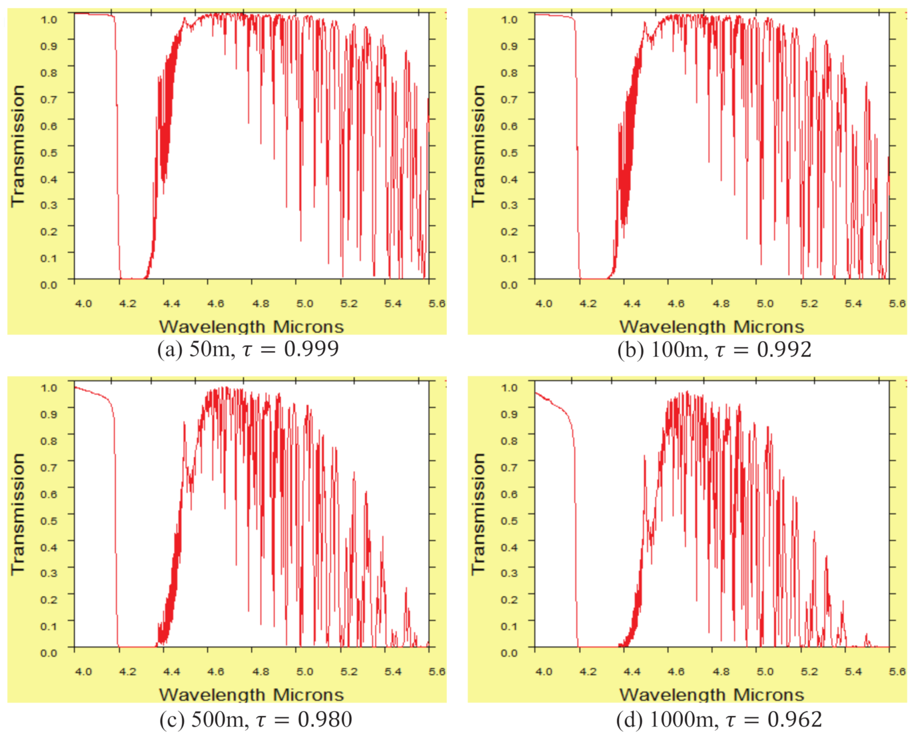
- can provide a feasible approximate solution in the upper MWIR band (4.2–5.6 m).
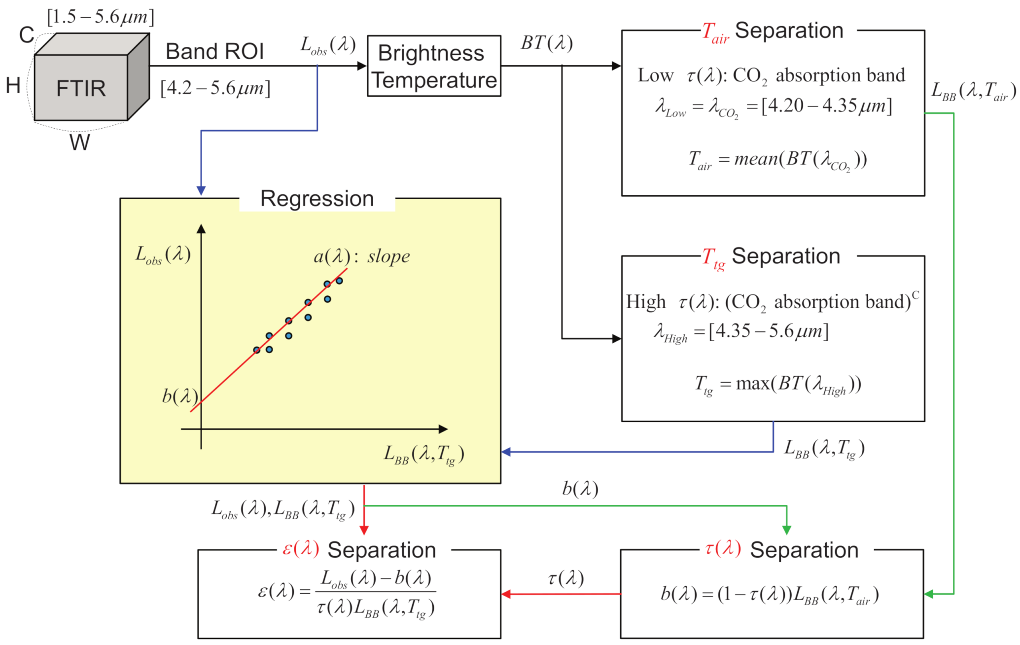
2. Proposed Method
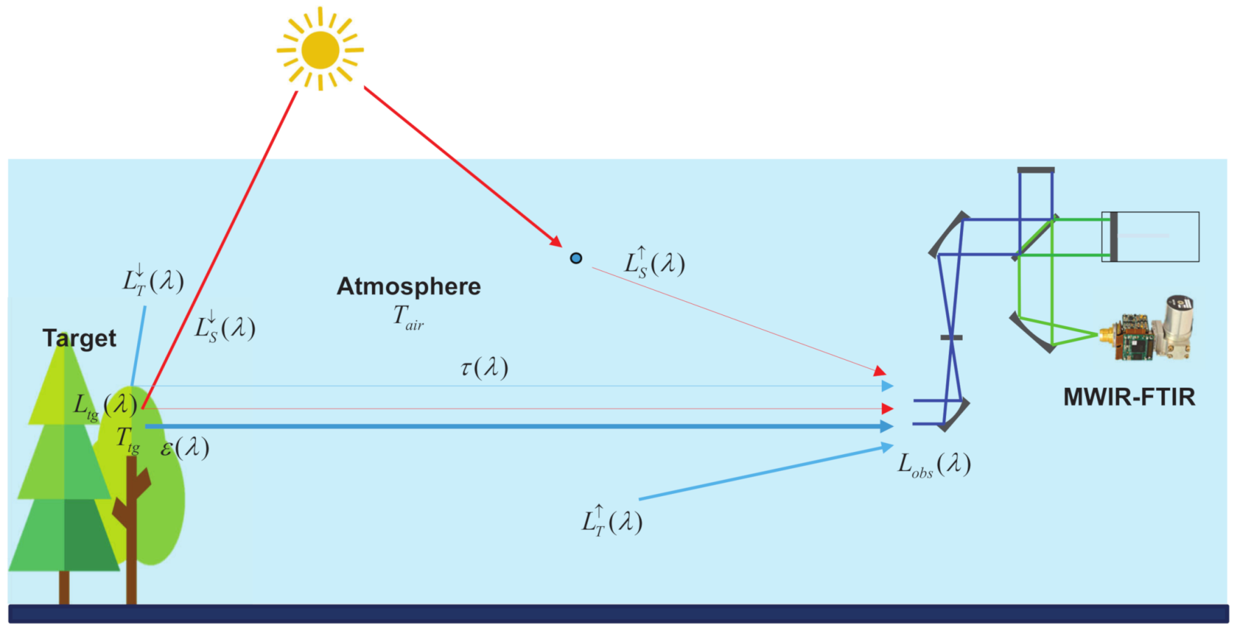
2.1. Basics of the Radiative Transfer Equation
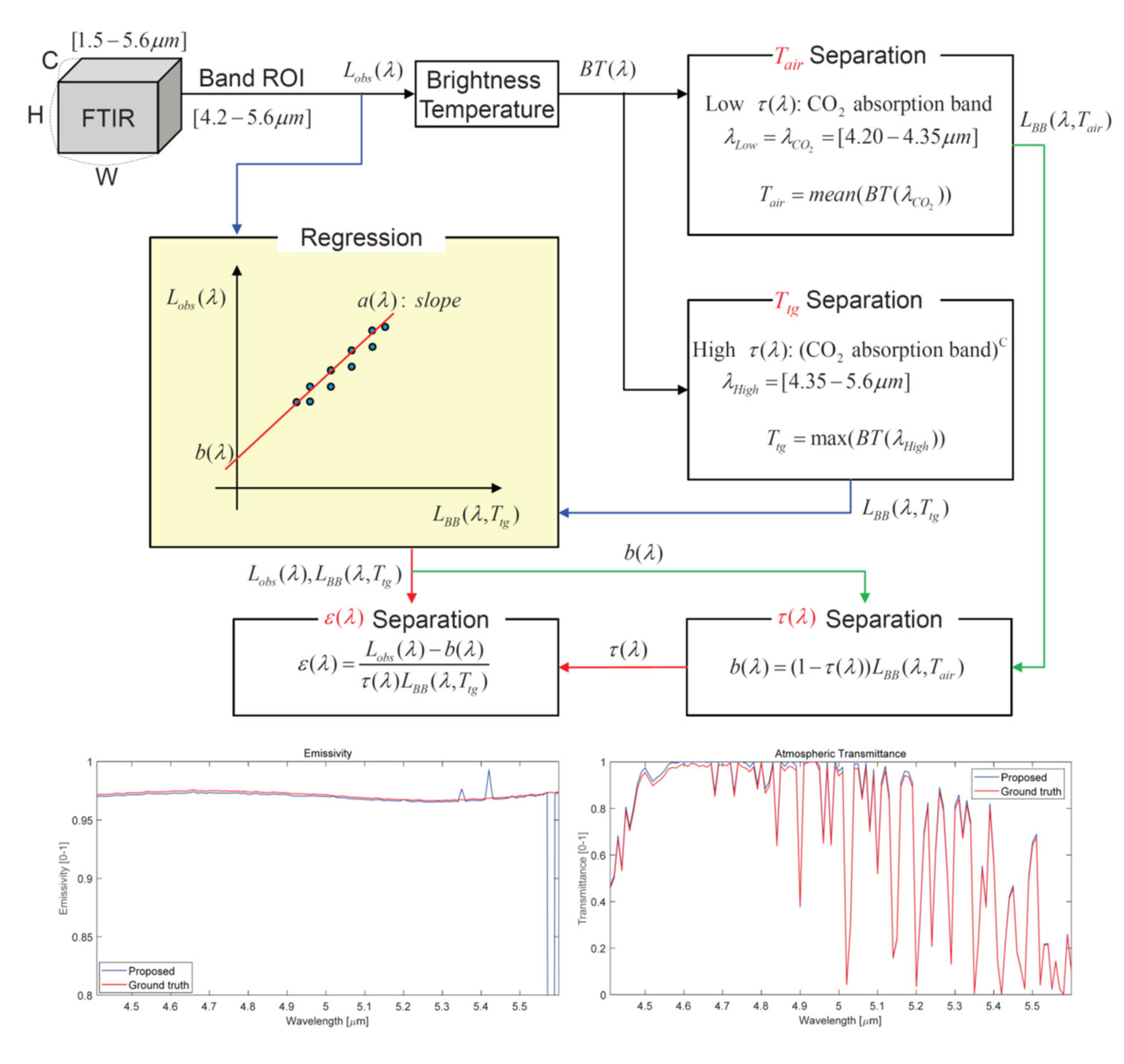
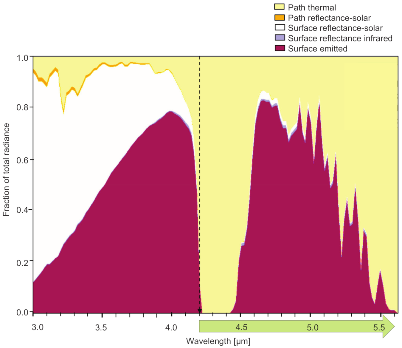
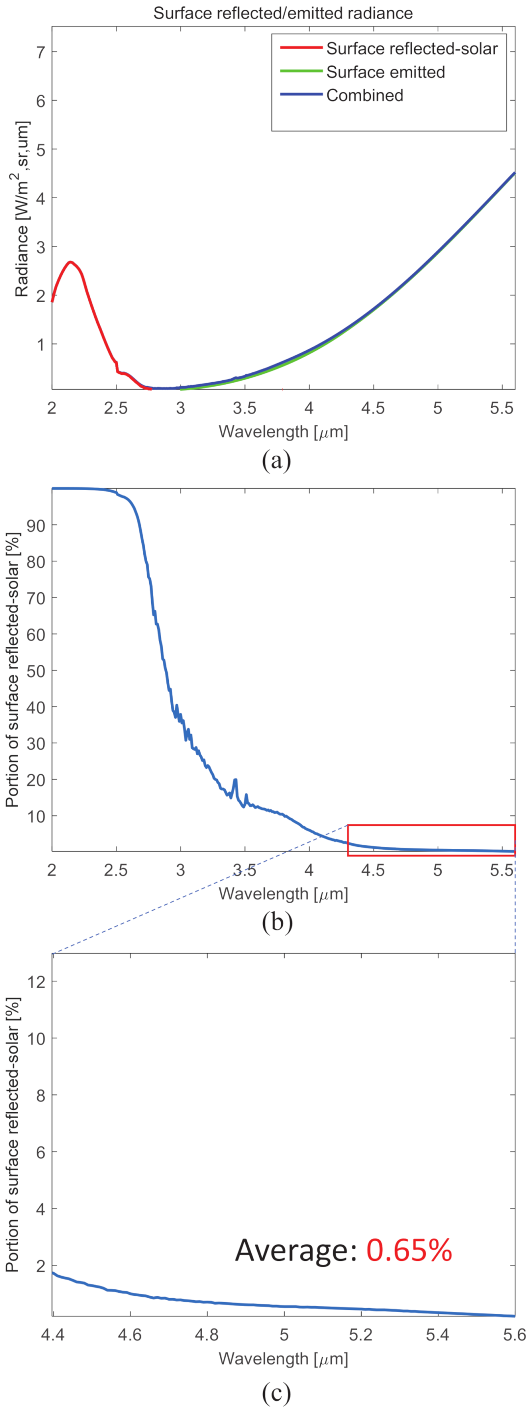
2.2. Proposed Approximation of the RTE in the Upper MWIR Band
2.3. Details of the Process
3. Experimental Results
3.1. Experiments Using Synthetic Hyperspectral Datasets
3.2. Experiments Using Real Hyperspectral Datasets
4. Conclusions
Author Contributions
Funding
Acknowledgments
Conflicts of Interest
References
- Gillespie, A.; Rokugawa, S.; Matsunaga, T.; Cothern, J.S.; Hook, S.; Kahle, A.B. A temperature and emissivity separation algorithm for Advanced Spaceborne Thermal Emission and Reflection Radiometer (ASTER) images. IEEE Trans. Geosci. Remote Sens. 1998, 36, 1113–1126. [Google Scholar] [CrossRef]
- Payan, V.; Royer, A. Analysis of Temperature Emissivity Separation (TES) algorithm applicability and sensitivity. Int. J. Remote Sens. 2004, 25, 15–37. [Google Scholar] [CrossRef]
- Li, Z.L.; Becker, F.; Stoll, M.P.; Wan, Z. Evaluation of Six Methods for Extracting Relative Emissivity Spectra from Thermal Infrared Images. Remote Sens. Environ. 1999, 69, 197–514. [Google Scholar] [CrossRef]
- Pivovarník, M.; Khalsa, S.J.S.; Jiménez-Muñoz, J.C.; Zemek, F. Improved Temperature and Emissivity Separation Algorithm for Multispectral and Hyperspectral Sensors. IEEE Trans. Geosci. Remote Sens. 2017, 55, 1944–1953. [Google Scholar] [CrossRef]
- Cui, J.; Yan, B.; Dong, X.; Zhang, S.; Zhang, J.; Tian, F.; Wang, R. Temperature and emissivity separation and mineral mapping based on airborne TASI hyperspectral thermal infrared data. Int. J. Appl. Earth Obs. Geoinf. 2015, 40, 19–28. [Google Scholar] [CrossRef]
- Neinavaz, E.; Skidmore, A.K.; Darvishzadeh, R. Effects of prediction accuracy of the proportion of vegetation cover on land surface emissivity and temperature using the NDVI threshold method. Int. J. Appl. Earth Obs. Geoinf. 2020, 85, 101984. [Google Scholar] [CrossRef]
- Zhong, Y.; Jia, T.; Zhao, J.; Wang, X.; Jin, S. Spatial-Spectral-Emissivity Land-Cover Classification Fusing Visible and Thermal Infrared Hyperspectral Imagery. Remote Sens. 2017, 9, 910. [Google Scholar] [CrossRef] [Green Version]
- Young, S.J.; Johnson, B.R.; Hackwell, J.A. An in-scene method for atmospheric compensation of thermal hyperspectral data. J. Geophys. Res. Atmos. 2002, 107, ACH 14-1–ACH 14-20. [Google Scholar] [CrossRef]
- Borel, C.C.; Tuttle, R.F. Recent advances in temperature-emissivity separation algorithms. In Proceedings of the 2011 Aerospace Conference, Big Sky, Montana, 5–12 March 2011; pp. 1–14. [Google Scholar] [CrossRef]
- Wang, H.; Xiao, Q.; Li, H.; Zhong, B. Temperature and emissivity separation algorithm for TASI airborne thermal hyperspectral data. In Proceedings of the 2011 International Conference on Electronics, Communications and Control (ICECC), Ningbo, China, 9–11 September 2011; pp. 1075–1078. [Google Scholar] [CrossRef]
- Adler-Golden, S.; Conforti, P.; Gagnon, M.; Tremblay, P.; Chamberland, M. Remote sensing of surface emissivity with the telops Hyper-Cam. In Proceedings of the 2014 6th Workshop on Hyperspectral Image and Signal Processing: Evolution in Remote Sensing (WHISPERS), Lausanne, Switzerland, 24–27 June 2014; pp. 1–4. [Google Scholar] [CrossRef]
- Wang, S.; He, L.; Hu, W. A Temperature and Emissivity Separation Algorithm for Landsat-8 Thermal Infrared Sensor Data. Remote Sens. 2015, 7, 9904–9927. [Google Scholar] [CrossRef] [Green Version]
- Romaniello, V.; Spinetti, C.; Silvestri, M.; Buongiorno, M.F. A Sensitivity Study of the 4.8 um Carbon Dioxide Absorption Band in the MWIR Spectral Range. Remote Sens. 2020, 12, 172. [Google Scholar] [CrossRef] [Green Version]
- Kim, S.; Kim, J.; Lee, J.; Ahn, J. AS-CRI: A New Metric of FTIR-Based Apparent Spectral-Contrast Radiant Intensity for Remote Thermal Signature Analysis. Remote Sens. 2019, 11, 777. [Google Scholar] [CrossRef] [Green Version]
- Griffin, M.K.; Hua, K.; Burke, H.; Kerekes, J.P. Understanding radiative transfer in the midwave infrared: a precursor to full-spectrum atmospheric compensation. Proc. SPIE 2004, 5425, 348–356. [Google Scholar] [CrossRef]
- Andrews, D. An Introduction to Atmospheric Physics; Cambridge Press: Cambridge, UK, 2000. [Google Scholar]
- Hohn, D.H. Atmospheric Vision 0.35 um < x < 14 um. Appl. Opt. 1975, 14, 404–412. [Google Scholar] [PubMed]
- Sobrino, J.; Li, Z.L.; Stoll, P.; Becker, F. Multi-channel and multi-angle algorithms for estimating sea and land surface temperature with ATSR data. Int. J. Remote Sens. 2004, 17, 2089–2114. [Google Scholar] [CrossRef]
- Driggers, R.G.; Friedman, M.H.; Nichols, J. Introduction to Infrared and Electro-Optical Systems; Artech House: Norwood, MA, USA, 2012. [Google Scholar]
- Eismann, M.T. Hyperspectral Remote Sensing; SPIE Press: Bellingham, WA, USA, 2012. [Google Scholar]
- Kim, S. Novel Air Temperature Measurement Using Midwave Hyperspectral Fourier Transform Infrared Imaging in the Carbon Dioxide Absorption Band. Remote Sens. 2020, 12, 1860. [Google Scholar] [CrossRef]
- Silvestri, M.; Romaniello, V.; Hook, S.; Musacchio, M.; Teggi, S.; Buongiorno, M.F. First Comparisons of Surface Temperature Estimations between ECOSTRESS, ASTER and Landsat 8 over Italian Volcanic and Geothermal Areas. Remote Sens. 2020, 12, 184. [Google Scholar] [CrossRef] [Green Version]
- Willmott, C.J.; Matsuura, K. Advantages of the mean absolute error (MAE) over the root mean square error (RMSE) in assessing average model performance. Clim. Res. 2005, 30, 79–82. [Google Scholar] [CrossRef]
- Gagnon, M.A.; Gagnon, J.P.; Tremblay, P.; Savary, S.; Farley, V.; Guyot, É.; Lagueux, P.; Chamberland, M. Standoff midwave infrared hyperspectral imaging of ship plumes. Proc. SPIE 2016, 9988, 998806. [Google Scholar] [CrossRef]
- Shamsipour, A.; Azizi, G.; Ahmadabad, M.K.; Moghbel, M. Surface temperature pattern of asphalt, soil and grass in different weather condition. J. Biodivers. Environ. Sci. 2013, 3, 80–89. [Google Scholar]


Publisher’s Note: MDPI stays neutral with regard to jurisdictional claims in published maps and institutional affiliations. |
© 2021 by the authors. Licensee MDPI, Basel, Switzerland. This article is an open access article distributed under the terms and conditions of the Creative Commons Attribution (CC BY) license (http://creativecommons.org/licenses/by/4.0/).
Share and Cite
Kim, S.; Shin, J.; Kim, S. AT2ES: Simultaneous Atmospheric Transmittance-Temperature-Emissivity Separation Using Online Upper Midwave Infrared Hyperspectral Images. Remote Sens. 2021, 13, 1249. https://doi.org/10.3390/rs13071249
Kim S, Shin J, Kim S. AT2ES: Simultaneous Atmospheric Transmittance-Temperature-Emissivity Separation Using Online Upper Midwave Infrared Hyperspectral Images. Remote Sensing. 2021; 13(7):1249. https://doi.org/10.3390/rs13071249
Chicago/Turabian StyleKim, Sungho, Jungsub Shin, and Sunho Kim. 2021. "AT2ES: Simultaneous Atmospheric Transmittance-Temperature-Emissivity Separation Using Online Upper Midwave Infrared Hyperspectral Images" Remote Sensing 13, no. 7: 1249. https://doi.org/10.3390/rs13071249