Article

Extensive Evaluation of a Continental-Scale High-Resolution Hydrological Model Using Remote Sensing and Ground-Based Observations

1
State Key Laboratory of Remote Sensing Science, Faculty of Geographical Science, Beijing Normal University, Beijing 100875, China
2
China Institute of Water Resources and Hydropower Research, State Key Laboratory of Simulation and Regulation of Water Cycle in River Basin, Beijing 100038, China
3
China Institute of Water Resources and Hydropower Research, Beijing 100038, China
*
Author to whom correspondence should be addressed.
Remote Sens. 2021, 13(7), 1247; https://doi.org/10.3390/rs13071247
Submission received: 29 January 2021 / Revised: 20 March 2021 / Accepted: 21 March 2021 / Published: 25 March 2021

Abstract

:
Extreme hydrologic events are getting more frequent under a changing climate, and a reliable hydrological modeling framework is important to understand their mechanism. However, existing hydrological modeling frameworks are mostly constrained to a relatively coarse resolution, unrealistic input information, and insufficient evaluations, especially for the large domain, and they are, therefore, unable to address and reconstruct many of the water-related issues (e.g., flooding and drought). In this study, a 0.0625-degree (~6 km) resolution variable infiltration capacity (VIC) model developed for China from 1970 to 2016 was extensively evaluated against remote sensing and ground-based observations. A unique feature in this modeling framework is the incorporation of new remotely sensed vegetation and soil parameter dataset. To our knowledge, this constitutes the first application of VIC with such a long-term and fine resolution over a large domain, and more importantly, with a holistic system-evaluation leveraging the best available earth data. The evaluations using in-situ observations of streamflow, evapotranspiration (ET), and soil moisture (SM) indicate a great improvement. The simulations are also consistent with satellite remote sensing products of ET and SM, because the mean differences between the VIC ET and the remote sensing ET range from −2 to 2 mm/day, and the differences for SM of the top thin layer range from −2 to 3 mm. Therefore, this continental-scale hydrological modeling framework is reliable and accurate, which can be used for various applications including extreme hydrological event detections.

Graphical Abstract

1. Introduction

Climate change and human activities impose substantial influences on hydrological cycles and water resources, resulting in considerable challenges in multi-scale hydrological research [1]. A lot of research is devoted to solving practical issues, such as detecting and predicting floods and droughts, managing water resources, and designing water supply infrastructures at finer scales [2]. As an effective solution, a high-quality hydrological modeling is key to the improved understanding of land–atmosphere interactions, surface and subsurface interactions, water quality, and human impacts on the terrestrial water cycle [3], which can serve as a benchmark for evaluating extreme events and for preventing record-setting disasters in advance [4,5]. Developing a reliable and accurate hydrological modeling is also recognized as important for understanding the implications of climate change [6] and improving the ability of scientists to narrow uncertainties in water resources management [7]. The development of high-quality hydrological modeling requires extensive validations between simulations and reference datasets (e.g., ground-based observations and remote sensing products). Ground-based observations record continuous values of the water, energy, and carbon budgets. Remote sensing products can provide detailed information on hydrological and biogeochemistry fluxes and states over a variety of scales and resolutions. Therefore, both ground-based and remotely sensed datasets are useful for model evaluations.
At present, hydrological modeling is usually implemented at various spatial and temporal resolutions [8,9] across different regions, such as Mexico [6], Texas [4], Yellow River basin [10], Xijiang River basin [11], and the Mississippi watershed [7,12,13]. Hydrological modeling has also been used by a variety of studies to analyze the effects of diversified climate conditions and land surface properties on the water cycle [14,15,16,17]. In recent decades, many devastating natural disasters occurred frequently worldwide and in China due to global climate change [18,19,20]. The intensification of droughts and floods is having a critical negative impact (i.e., economic losses, agricultural destruction) in China [21]. Therefore, an accurate and reliable hydrological modeling at a continental scale with long-term, high-resolution, and acceptable performance is urgently needed to identify and monitor the underlying processes and intensities of hydrological extremes [22] and to reflect the regional details of climate change patterns [23].
However, there are difficulties in developing high spatial-resolution hydrological modeling in China with respect to meteorological forcings, soil and vegetation datasets, and model evaluation. First, meteorological forcing data hold substantial uncertainties, because ground-based observation stations are limited in China. Only ~750 meteorological stations for collecting data (which may be combined with remote sensing datasets) have been commonly used to generate different resolutions of forcing data [15,18,24], and these datasets are suitable for modeling at coarse resolutions (>10 km) rather than at high resolutions. The coarse-resolution model simulations are not able to adequately address critical scientific issues associated with the water cycle [3] or to describe the hydrological processes and water dynamics at a small scale (<10 km). Second, estimating model parameters presents a great challenge because the climate, soil, and land cover conditions are highly heterogeneous over the 9.6 million km2 area of China [24]. Soil properties are fundamental inputs for the hydrological model which determine the soil water movements and thus affect other surface and subsurface hydrological fluxes and states. Soil properties (e.g., hydraulic conductivity) have high spatial variability, even at very small scales [25,26], therefore some of the physical model parameters cannot be accurately estimated by previous studies and are usually treated as random [27]. Therefore, incorporating a high-quality and high-resolution soil dataset is essential for hydrological model configuration. Third, ground-based hydrological stations are extremely scarce in most basins, and hydrological datasets are insufficient for model calibration and validation. Thus, in some studies, model parameters were calibrated using limited streamflow data, while evapotranspiration (ET) and soil moisture (SM) states have not been well evaluated [7,28]. Finally, remote sensing (RS) data can serve as hydrological model inputs; however, RS data have not been incorporated into hydrological modeling by previous studies, although they have the potential to improve model performance [29].
In this study, we attempt to develop a high-quality hydrological modeling framework for China featured by long-term and fine spatial resolution of 0.0625° (~6 km), being incorporated with a newly released soil dataset and fully evaluated against observations and remote sensing products. The framework is based on a land surface hydrological model, (i.e., the variable infiltration capacity (VIC)) [30,31]. Many previous studies set up the VIC model at a spatial resolution of 0.25° or 0.5 ° over China with input forcing data from the 750 meteorological stations to analyze hydrologic states and fluxes (e.g., soil moisture, runoff) under climate change [11,32,33] and to develop hydrologic state and flux datasets. In this study, the VIC model is driven by meteorological forcing data that are generated based on data from relatively high-density ground-based stations (2481 stations), nearly tripling the number of meteorological stations when compared with other studies [14,15,34]. The soil parameters of the VIC are updated based on a newly developed soil dataset for China, which provides an improved representation of hydrological and biogeochemical characteristics and is capable of being incorporated into land models [35,36]. The features in this framework include: (1) an effective scheme is employed to estimate model parameters for ungauged basins, which can be extended to another ungauged area [37,38]; (2) the simulated runoff, ET, and SM are extensively evaluated using ground-based measurements and RS data products.
This hydrological modeling framework has wide applications and potential extensions. The simulated hydrological flux and state variables are useful for understanding long-term climatic changes and water resource security at various scales. Furthermore, compared with other researches aiming to produce the state-of-the-art terrestrial hydrological dataset [15,39], our study mainly focuses on developing and evaluating a hydrological modeling framework that can be extended to couple with the China Meteorological Administration Land Data Simulation System (CLDAS), which provides real-time meteorological inputs and SM conditions at the same resolution (i.e., 0.0625°) [40]. This hydrological modeling, if driven by high-quality and real-time inputs from CLDAS, may improve the performance for real-time hydrological processes and accuracy for extreme hydrologic detection.
In the next section, we describe the structure of the VIC model, including its forcing data and parameters, and present the method of calibration and parameter transfer. In Section 3, we describe the evaluation of model performance over China. We discuss its reliability, potential, and limitations in Section 4, and in Section 5 we present our conclusions and thoughts on future works.

2. Materials and Methods

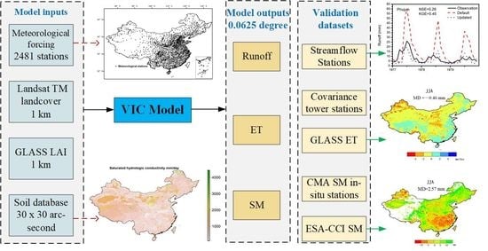
2.1. Hydrological Model

The VIC model is a distributed and physically-based model that solves the surface energy and water balance [30,31]. It simulates SM, ET, snowpack, surface runoff, baseflow, and other hydrological variables in daily or sub-daily time steps. Each grid cell is partitioned into multiple vegetation types, and the soil column has three soil layers, where each layer characterizes the dynamic response of soil to climatic conditions. The VIC model characterizes multiple land cover types. Each vegetation type has a leaf area index (LAI), minimum stomatal resistance, roughness length, displacement length, and relative fraction of the root [41].
This model was selected for use in this study due to three main advantages: (1) a conceptual large-scale hydrological model was used that allows the spatial representation of gridded topography, infiltration rate, soil properties, climate variables, and land covers, which are important factors in modeling runoff under spatially heterogeneous conditions [42]; (2) both infiltration and saturation excess runoff generation mechanisms were considered in the model, making it suitable for application to both arid and humid regions; (3) it was able to simulate snow and frozen soil processes, which are necessary for the Tibet Plateau. Finally, the VIC model has also been shown to represent land surface hydrologic processes well in numerous studies [29,43] and has been used from global [29,44] to river basin scales [45] to assess water resources, land-atmosphere interactions, and overall hydrological budgets.

2.2. Data for Model Inputs

2.2.1. Meteorological Forcing Data

The VIC model is driven by historical meteorological forcing, including precipitation (mm), minimum and maximum temperature (°C, and wind speed (m/s). We run the model in daily time steps from 1970–2016 in a water-balance mode. All of the forcing data were produced by interpolating ground-based observations from the 2481 meteorological stations in China (Figure 1a, Table 1), which were obtained from the China Meteorological Administration (CMA). These data were interpolated into a gridded dataset (at the resolution of 0.0625°) by an inverse distance weighting (IDW) method. There are a few alternative interpolation methods, e.g., Kriging, the synergraphic mapping system (SYMAP) algorithm [46], but here we used IDW because it is a commonly used method, and the same interpolation method for generating gridded forcing data has been successfully applied in previous VIC simulations [14,47,48]. At least five stations around the target grid cell were searched to conduct this interpolation. A lapse rate of −6.5 °C km 1 with respect to the elevation difference between the station and the target grid cell was used to reflect the decrease in temperature with increasing elevation.

2.2.2. Vegetation Dataset

Vegetation data needed for VIC simulations included land cover (LC) types and associated vegetation parameters. Details of the LC types were originally created by merging a number of Land Satellite Thematic Mapper (Landsat TM) images [49], with a spatial resolution of 1 km. There are 12 types of LC distributed across China. Based on these LC types, the fractional area of each vegetation type in a grid cell was calculated.
The parameters for each type of vegetation (e.g., the architectural resistance) are available from https://vic.readthedocs.io/en/master/Datasets/Datasets/, except for the LAI. The LAI reflects the amount of available leaf material, and thus, represents the canopy density and growth of vegetation, and influences the ET process [50]. The LAI data at a spatial resolution of 1 km were obtained from the eight-day composite Global Land Surface Satellite (GLASS) product between 2000 and 2015, and they were retrieved from the Moderate Resolution Imaging Spectroradiometer (MODIS) reflectance data (MOD09A1) using a general regression neural networks algorithm [51,52]. Hence, based on the LC maps and the LAI data, vegetation parameters are generated for use in the VIC simulations.

2.2.3. Soil Dataset

Soil datasets define the soil physical and chemical properties of grid cells. Integrating with reliable soil data is important to improve the quality of the hydrological processes modeling and the parameterization of hydrological models and especially in ungauged basins [53,54].
In this study, detailed information on the physical and chemical properties of soils were obtained based on a 30 × 30 arc-second-resolution soil characteristics dataset [35,36] derived by using the 1:1,000,000 Soil Map of China and 8595 representative soil profiles (Table 1). This dataset is specifically suitable for land surface models, so it can be incorporated into hydrological models to better represent the role of soils in hydrological and biogeochemical cycles in China. This soil dataset has 10 layers, which are aggregated to three layers for the same depth of the VIC model.
Four influential soil parameters (i.e., field capacity, wilting point, saturated hydraulic conductivity, and bulk density) for each of the three layers were obtained from the dataset of soil properties for land surface modeling over China [35,36] and then applied to the 0.0625° grid in this study. The saturated hydrologic conductivity ranged from 96.9 to 4440.2 mm/day in the top 10 cm layer. The bulk density ranged from 474.8 to 1487 kg/m3. The minimum and maximum values for the wilting point were 0.09 and 0.68 m3/m3, and the filed capacity ranged from 0.32 to 0.91 m3/m3, respectively. The other soil parameters, such as the thermal damping depth, bubbling pressure, surface roughness of bare soil, and snowpack were prescribed according to data from the Food and Agriculture Organization (FAO) of the United Nations (UN) dataset, which has been used by Nijssen, et al. [55] and Nijssen, et al. [56]. Particularly, the dataset from FAO has been successfully applied to construct modeling for China at a resolution of 0.25° [15], which is considered as the initial or default setting for model parameters in this study.

2.3. Data for Model Evaluation

2.3.1. Streamflow

The VIC model is first calibrated and validated using streamflow data. We obtain 29 stations of streamflow data from the Annual Hydrological Report for P.R. China (Figure 1b, Table 1). Since it is difficult to accurately evaluate the contributions of all human activities (e.g., irrigation, dam operations) on the water cycle in different regions, many previous studies directly used observation datasets without removing human influence in model evaluation. Therefore, the streamflow stations in our study were not adjusted to reflect unimpaired conditions. These stations are situated at the outlets of 29 sub-catchments that have different climatic and LC conditions. The data were partitioned into two groups: 20 stations of data for calibration and the remaining nine for model validation. The VIC simulated daily runoff in each month over the upstream grids of the control station were accumulated to be compared with the monthly streamflow observations. To highlight the advantages of updating the soil parameters, we conducted two simulations: one using the default soil parameters, which were directly downscaled from a 0.25° resolution modeling in the study by Zhang, et al. [15] (denoted as “default parameters”), and the other employed the updated values of soil parameters along with parameter calibration (denoted as “updated parameters”).

2.3.2. Evapotranspiration

ET is one of the largest terms in the global land surface water budget [57], and it was evaluated in this study using ground-based observations and an RS product. Ground-based observations of ET are obtained from eddy covariance towers (Table 1), which were assumed to capture ET flux at a footprint less than 1 km. To reduce the scale difference between the observations and the VIC simulation (~6 km), the stations near to the center of the target grid cell (<1 km) were selected, thus the ET observations from 33 covariance tower stations were employed to evaluate the modeling (Figure 1b). Instead of NSE, the root mean square error (RMSE) was calculated to evaluate the differences between the VIC simulated ET and the ground-based observations, because it is a widely used measure in ET and SM evaluations [58].
The RS ET product was from the Global Land Surface Satellite (GLASS). This product merges multiple sources of RS data to achieve reliable ET estimates [59,60,61,62]. Moreover, the GLASS ET was approximately equal in spatial resolution (0.05°) to the model in this study, and was therefore applicable to evaluate the VIC simulated ET.

2.3.3. Soil Moisture (SM)

SM plays an important role in the terrestrial hydrological cycle, and it is also related to agricultural droughts. SM data from 66 in-situ stations across China (Figure 1b, Table 1) were obtained from CMA. To guarantee the reliability of the validation results, we selected the stations that were near to the center of a target grid cell and cover a long measurement period. The RS SM data are available from the European Space Agency Water Cycle Multimission Observation Strategy and Climate Change Initiative projects (ESA-CCI SM). The ESA-CCI product provides relatively consistent and reliable information for SM worldwide [63] and has been successfully validated by a few studies [64,65].

2.4. Parameter Calibration and Transfer Scheme

2.4.1. Parameter Calibration

After all of the necessary input data for the model were collected and prepared, the VIC model was calibrated for the selected 20 basins and validated for the nine basins located in different climate zones (Figure 1b). Most basins were minimally affected by human activities, such as water extraction, irrigation, and water management. Seven of the most sensitive VIC model parameters were targeted for calibration in each basin separately, including the infiltration curve (b), the depths of the soil layers (d1, d2, d3), the maximum velocity of the baseflow (Dsmax), the fraction of the maximum baseflow velocity (Ds), and the fraction of the baseflow of the maximum SM where non-linear baseflow occurs (Ws). The first soil depth (i.e., d1) was usually defined as 10 cm. The parameters Dsmax, Ds, Ws, and d3 are influential for runoff and early season SM and ET since they govern water infiltration and baseflow generation [66]. The initial/default values of these sensitive parameters were obtained from Zhang, et al. [15] at a 0.25° resolution and then were directly downscaled to a 0.0625° resolution using the nearest-neighbor mapping method. The calibration is conducted by searching for the best combination of the seven parameters to match the simulations with the hydrograph observations.
Four widely-used metrics were employed to evaluate model performance: (1) the correlation coefficient (R), (2) the Nash-Sutcliffe efficiency (NSE), (3) the relative error (bias, %) between observations and simulations, and (4) the Kling–Gupta efficiency (KGE) [67].
R = ( Q i , o b s Q o b s ¯ ) ( Q i , s i m Q s i m ¯ ) ( Q i , o b s Q o b s ¯ ) 2 ( Q i , s i m Q s i m ¯ ) 2
NSE = 1 ( Q i , o b s Q i , s i m ) 2 ( Q i , o b s Q o b s ¯ ) 2
Bias ( % ) = ( Q s i m ¯ Q o b s ¯ ) Q o b s ¯ × 100 %
K G E = 1 ( R 1 ) 2 + ( α 1 ) 2 + ( β 1 ) 2
where Q i , o b s is the observed flow in the i month, Q i , s i m is the respective i th simulated flow from the model, Q s i m ¯ and Q o b s ¯ are the observed and simulated mean monthly discharges for the calibration period, respectively, α is the ratio between the standard deviations of simulated and observed values, and β is the ratio between the mean simulated and mean observed flows.
For each grid cell in the calibrated basins, an adjustment factor (Adj_factor) can be defined as:
A d j _ f a c t o r = P A R f i n a l P A R i n i t i a l
where PARfinal and PARinitial are the final and the initial estimates of the parameter, respectively. Based on this adjustment factor, the estimates of parameters in the calibrated basins were transferred to the ungauged basins.

2.4.2. Parameter Transfer

The estimated parameters from gauged basins were transferred to ungauged basins based on their climatic similarity. Specifically, the area of China is divided into nine large river basins (Figure 2) according to topographic and LC conditions. As the VIC model parameters are closely related to physical and climatic characteristics of basin properties, such as LC and meteorological factors, we overlayed the river basins with climate zones to define a climatic similarity, as described by Xie, et al. [14]. Based on the climatic similarity and the adjustment factor (Adj_factor), the estimated parameters in the calibrated basins were transferred to the ungauged/uncalibrated basins. The 20 independent, calibrated basins were located in different climate zones and designed to estimate the parameters in the uncalibrated, climate-related areas. Seven climatic zones in China, as defined based on the Köppen classification criteria [68], are shown in Table 2 and Figure 2. The parameter transfer scheme has been successfully used by Xie, et al. [14], and it is briefly described as follows:
(1) The adjustment factors in each calibrated basin were used to adjust parameters in uncalibrated basins;
(2) The rainy climate zone was further divided into three parts according to basins of the Huai River, Yangtze River, and Pearl River, as C1, C2, and C3, respectively;
(3) The tropical climate zone has similar climatic characteristics to the Pearl River basin. Therefore, the parameters for the tropical climate zone were set to the same adjustment values as C3;
(4) Parameters of southeastern basins were used as the equivalent multiple as the Yangtze River basin C2;
(5) The Dc climate zones cover two different regions in northeastern and southwestern China (Dc east and Dc west). Therefore, the parameters in Dc east and Dc west were adjusted using the same multiples from the related Da and E zones, respectively.

3. Results

3.1. Runoff Calibration and Validation

Figure 3 presents the monthly discharge of the simulations from the default and calibrated/updated parameters and the observations over nine river basins, which were selected to be regionally representative and distributed among diverse climates. The model performance was considerably better when using the updated parameters rather than the default parameters (Section 2.4.1). For most basins, the simulations with the default parameters tended to have higher discharges, especially overestimating the peak flow during summers, such as in Phujym, Jilin, Heishiguan, and Tsuuang. In contrast, the simulation with the updated parameters was able to capture the peak flow avoiding overestimation. For the basins with small rainfall and runoff (i.e., Shetang, Maojiahe, and Tsyamusy), the simulations with the default parameters do not match the observations well during the low-flow seasons, but the performance was substantially improved after parameter update and calibration. Overall, the comparisons revealed that the runoff dynamics were well captured after parameter update and calibration, and consequently the model performance was improved relative to the simulation with the default parameters.
Table 3 lists the model performance for each basin after calibration and validation. Most of the calibrated basins had high R and NSE values over 0.70. Most of the KGE values were higher than 0.40. The relative bias presented here was generally within 20%. The simulations of basins located in southern China (e.g., C1, C2, and C3), which usually receive abundant rainfall and experience substantial runoff throughout the entire year, tend to have better agreements with observations than those in northern China (e.g., Da, Db, and Bk). In general, the calibration improves the model performance, although, in some basins, such as Dingjiagou and Phujym, the results were unsatisfactory. A possible reason for such a discrepancy is that the VIC model is unable to capture the impact of human activities, such as agricultural irrigation. As an external water input, agricultural irrigation may significantly affect the surface runoff and baseflow, leading to the discrepancy of the runoff between simulations and observations over irrigated regions.
The simulated streamflow was validated for the remaining nine basins. Compared with the calibration process, six validation basins covering two climate zones, i.e., Da and Db, were used to examine the performance of the parameter transfer approach. Overall, the validation results (Table 3) were similar to the calibration statistics. The R, NSE, KGE, and bias values for the validation period ranging from ~0.65–0.91, ~0.31–0.87, ~0.01–0.86, and ~4.29–40.5%, respectively. The Zhangjiashan Basin had a relatively high bias, mainly because of only two years of observation data available for validation. The best performance was found in the Hengshi Basin, while the worst was in the Chiling Basin.

3.2. ET Evaluation

The statistics of the comparison between the ET simulations and the observations are shown in Figure 4. The VIC model performed well and showed reasonable consistency at the eddy covariance tower stations with respect to daily ET, with most R values being greater than 0.5. The RMSE values range between 0.6 mm and 3.6 mm/day. With respect to bias, many stations located in central China have values between −60% and 20%. Poor performances appear at a few stations possibly due to the scale difference between the simulations and the observations [69]. Specifically, the observations with an eddy covariance tower represent the ET flux of the scale less than 1 km, while the VIC model produces the hydrological state and flux at the scale of 6 km in this study, although the eddy covariance tower was near to the center of the target grid cell. Besides, the VIC model was only able to simulate the natural conditions rather than the human-impact conditions which may cause uncertainties during comparisons. As a whole, the strong correlations regarding high R values and the small RMSEs indicate that the ET simulations are generally acceptable. Figure 5a summarizes the comparisons of the ET between the simulations and the observations. It provides a way of graphically summarizing how closely a pattern (or a set of patterns) matches observations. In the Yellow River basin (Figure 5a), for example, the pattern correlation with observations was about 0.6. The centered RMSE was proportional to the distance to the point on the x-axis identified as “1.0”. The isoline contours represent the RMSE, and it can be seen that in the Yellow River basin, the centered RMSE was about 0.8 mm. The standard deviation of the simulated pattern was proportional to the radial distance from the origin. The standard deviation was about 0.6 for the Yellow River Basin. According to the R values, the VIC model showed better results for Hai River, Huai River, and Southeast River than those for the other basins. The Southwest River basin had the lowest R value due to the small number of meteorological stations in this area as shown in Figure 1a.
The ET simulation was further evaluated with the RS datasets. As shown in Figure 6, the average monthly ET from the VIC simulations showed comparatively good agreement with the GLASS ET for each basin. The Southeast River Basin and the Pearl River Basin had the highest ET flux, while the Inland River Basin presented the lowest ET due to the inadequate precipitation throughout the year. Figure 7 shows the seasonal changes and the differences between the VIC simulated ET and the GLASS ET. The VIC simulated ET was larger than the GLASS in southeastern China and lower in the other areas. The differences range from −2 to 2 mm/day, which were partly attributable to the different temporal resolutions (the GLASS ET had a temporal resolution of eight days). However, the average difference for the four seasons was only about −0.36 mm/day, and thus the VIC simulated ET was consistent with the RS products, implying an acceptable performance for the model in this study.

3.3. SM Evaluation

SM is also evaluated with the ground-based observations and the RS products. Figure 4 and Figure 5b show the performance of the top 10-cm SM estimates against the ground-based SM observations. The R values for most stations were higher than 0.6 and the RMSEs were less than 12 mm. There was a pattern in which stations with high R values (> 0.7) usually had considerably low RMSEs, indicating R and the RMSE were not two independent indicators. The best results were shown in the Pearl River basin with the highest R value (~0.85) among the nine regions. The modeling presents a poor performance at several stations, potentially because of the differences in temporal (10-day for observations and daily for simulations) and spatial resolutions. The errors for the central basins, such as Hai River and Yellow River, may be caused by the effects of human activities (e.g., agricultural irrigation) on hydrological processes. Overall, given the high R values and the low RMSEs for most stations, the comparisons of the two SM datasets demonstrate that they match reasonably well.
The ESA-CCI SM product was used to further evaluate the SM results from the spatial perspective. As shown in Figure 8, the magnitudes of simulated SM in the top layer matched well with the ESA-CCI product. SM tends to be high in the south region (e.g., Pearl River, Southeast River) and the VIC modeling can successfully capture the spatial pattern. Figure 9 describes the differences between the simulations and the ESA-CCI product. Relatively large differences in winter (December–February) could be found in southwestern China. The opposite pattern appeared in summer (June–August), with high differences in southeastern China. Slight differences between simulations and the ESA-CCI product were found in spring (March–May), with high values in the Yangtze River Basin. In autumn (September–November), the southern region was covered by high differences values, which was distinctly different from northern China. We should mention that the ESA-CCI SM product holds uncertainties due to its scaling and merging algorithms [65], and the product performs better over grassland than cropland and urban areas in China [70]. These results indicate that the VIC model with properly calibrated parameters provides satisfactory simulations of runoff, ET, and SM.

4. Discussion

4.1. Reliability of the Modeling

In this study, we developed a hydrological modeling framework for runoff, ET, and SM at a 0.0625° spatial resolution across China from 1970–2016. A few features ensure the reliability of the modeling framework. First, it employs gridded forcing datasets that are produced by interpolating observations from 2481 meteorological stations across China, in contrast to the ~750 stations that have been commonly used in many studies for China. Based on our previous modeling study over China using 752 meteorological stations to drive the VIC model, the simulated SM shows a lower correlation coefficient (<0.4) with the SM observations in the western portion of China. Therefore, increasing the meteorological stations can substantially improve model performance. Second, the parameter transfer scheme based on the climactic similarity is used to calibrate the VIC empirical parameters in ungauged basins. Physical soil parameters, moreover, which are essential in the VIC modeling, are adopted from the newly released soil datasets of Dai, et al. [35] and Shangguan, et al. [36] to improve the reliability of hydrological modeling. Third, our study uses adequate ground observations and RS data to perform extensive evaluation regarding runoff, ET, and SM. In contrast, most of the other studies have only validated streamflow [4,6,14], which may not guarantee the reliability for other hydrological variables, such as ET and SM.
A few other studies constructed national-scale hydrological modeling for China (e.g., Xie, et al. [14]; Gou, et al. [71]). Recent work by Miao and Wang [39] produced land surface fluxes for China using the same VIC modeling, and their work also illustrated the advantages of the forcing data generated from the 2400 meteorological stations and the soil parameters from Dai, et al. [35] and Shangguan, et al. [36]. Our work employed an effective parameter transfer scheme and the modeling was evaluated using streamflow data from gauge observations. Moreover, the modeling in this study has a relatively fine spatial resolution (0.0625° vs 0.25° in Miao and Wang [39]), which is beneficial to detect extreme hydrological events and to couple with the CLDAS. Therefore, this high-resolution hydrological modeling could be extended for relevant applications.

4.2. Potential Extension with CLDAS and RS Data

The CLDAS is a system that produces high-quality meteorological forcing and SM conditions over China at a 0.0625° resolution and in hourly time steps (Shi et al., 2011). Three land surface models are included in the current version of the CLDAS-V2.0 (i.e., CLM3.5, Noah-MP, and CoLM). In terms of the Global Land Data Assimilation System (GLDAS) [72] and the National Land Data Assimilation System (NLDAS) [73], the VIC model is considered to fully simulate hydrological processes.
In this study, the developed hydrological modeling framework based on VIC has the same resolution as the CLDAS, and it is easy to couple with the CLDAS. Therefore, this study provides an opportunity for the CLDAS to be combined with hydrological modeling to better enhance its services for extreme events analysis.
Based on the high-quality and high-density drivers from the CLDAS, the VIC modeling framework developed in this study could be applied to real-time hydrological process estimation across China, and then offer an effective guide to detecting real-time flood and drought events. Furthermore, the RS data, such as LAI, albedo, and shortwave radiation, can also be merged into the VIC to improve the model performance by considering the energy balance.

4.3. Limitations and Future Works

The VIC model is driven by 2481 meteorological stations, while the station density is low for the western part of China, which could cause uncertainties for simulations. To address this issue, one option is to use remote sensing products, such as GLASS, TRMM (Tropical Rainfall Measuring Mission), as the model forcing dataset. As shown in Section 3, the hydrological simulations are validated with the in-situ observations and the RS data over such a large region. However, with the exception of two stations, all of the streamflow stations only have the data records for the periods before 1990. The ET and SM observation stations are mostly distributed in North China and are scarce in the northwest of China. Furthermore, for the large-scale modeling research, the spatial heterogeneity in vegetation and soil parameterizations over small basins tends to be averaged out. Given the highly nonlinear features between vegetation/soil parameters and hydrologic processes, global and regional simulations tend to be biased and are not comparable to point observations, leading to uncertainties in model validation. Additionally, we calibrate the most sensitive six parameters of the VIC model (b, d2, d3, Dsmax, Ds, and Ws), while the other parameters are not calibrated. For example, the wintertime LAI and canopy fraction have a strong influence on variations in the snow water equivalent [66]. The in-situ observations of ET and SM are typically representative of the situation in a very small area around the measurement sites, thus the comparisons between ET, SM observations, and simulations at grid cell may cause certain uncertainties. We should mention that the RS products of ET and SM hold uncertainties due to their scaling and merging algorithms [65], leading to the mismatch for the model evaluation. Therefore, further efforts are needed to reduce uncertainties from model parameters and to improve the accuracy and application of the RS products, and to enhance the support of ground-based observation networks.
This study improves the spatial resolution of hydrological modeling to ~6 km across China, which is just one step toward further increasing the resolution. The modeling needs to be improved to reach a so-called hyperresolution (~1 km or finer), which is currently one of the “grand challenges” in the hydrology community [3]. Moreover, as hydrological processes generally evolve over various temporal scales, from minute to daily time steps, future studies should also focus on developing hydrological modeling with finer temporal resolutions [74]. However, the modeling in our study is conducted roughly, at a daily time step, due to the limitations of the forcing data. Hourly or smaller time step data can capture more detailed processes, such as flash floods, infiltration, and pore flow [75]. Furthermore, the achievement of high-spatial and temporal-resolution modeling not only requires the resolution to increase, but also involves the development of hydrological models to consider more physical processes that are consistent with such high resolutions, including lateral flow, agricultural irrigation, urbanization effect, glacier and snow process in high altitudes [47,76,77], and efficient runoff routing algorithms [29,78,79,80].

5. Conclusions

In order to address fundamental issues associated with extreme hydrologic events of environmental changes, we develop a long-term and 0.0625° resolution hydrological modeling incorporated with newly released soil property dataset and a remotely sensed vegetation dataset for China using the VIC model and evaluate for the period from January 1, 1970 to June 30, 2016. The modeled runoff, ET, and SM are fully evaluated against datasets from in-situ stations and RS products temporally and spatially. The modeled runoff results are significantly improved after parameter calibration and transfer using a climatic similarity scheme. The R and NSE values for streamflow of most calibrated and validated basins are greater than 0.70, and the relative biases are generally below 20%. The simulations of humid regions, such as the Yangtze River Basin, tend to agree better with observations than those of arid regions. The simulated ET and SM are also validated against ground-based observations and RS products. The R and RMSE values for ET and SM are quite acceptable. The simulated ET and SM and the RS products (i.e., GLASS, ESA-CCI) are consistent across spatial and temporal distributions. Therefore, such a full evaluation for the hydrological state and fluxes guarantee that this modeling has an improved performance relative to earlier modeling practices, thus can be used for continental-scale applications (e.g., extreme hydrologic events evaluation). Furthermore, the model parameters transfer scheme used in this study can be extended to other regions without ground-based observations for model calibration.
The modeling framework over a large domain generally involves many aspects, including the improvement of model physical processes relevant to a fine-scale (e.g., lateral flow agricultural irrigation, and urbanization effect). The development of a global hyper-resolution (on the order of 1 km) model is still a grand challenge to the community. This study does not improve model physical processes, but it makes a step forward for a continental-scale modeling with a relatively high resolution. This is the first time that hydrological states and fluxes at a 0.0625° spatial resolution are produced and extensively validated for China, and they are freely available to analyze multi-scale hydrological conditions. After this evaluation, the model is expected to be coupled with the CLDAS. Additional efforts are needed to improve the hydrological modeling by including more physical processes, and developing more model forcing datasets and advanced parameter calibration techniques.

Author Contributions

Conceptualization, B.Z. and X.X.; methodology, X.X.; validation, B.Z. and Y.Y.; data curation, C.L., T.L., Y.Y., K.J., and Y.W.; writing—original draft preparation, B.Z.; writing—review and editing, X.X.; visualization, X.X.; supervision, X.X.; project administration, X.X.; funding acquisition, X.X. All authors have read and agreed to the published version of the manuscript.

Funding

This study is supported by grants from the National Key Research and Development Program of China (NO.2016YFA0600104, No. 2016YFC0401404) and the National Natural Science Foundation of China (No. 41971030, 41601569).

Acknowledgments

We would like to thank the three anonymous reviewers and the editors for their constructive comments and careful language editing.

Conflicts of Interest

The authors declare no conflict of interest.

References

  1. Devia, G.K.; Ganasri, B.P.; Dwarakish, G.S. A Review on Hydrological Models. Aquat. Procedia 2015, 4, 1001–1007. [Google Scholar] [CrossRef]
  2. Kirchner, J.W. Getting the right answers for the right reasons: Linking measurements, analyses, and models to advance the science of hydrology. Water Resour. Res. 2006, 42. [Google Scholar] [CrossRef]
  3. Wood, E.F.; Roundy, J.K.; Troy, T.J.; van Beek, L.P.H.; Bierkens, M.F.P.; Blyth, E.; de Roo, A.; Döll, P.; Ek, M.; Famiglietti, J.; et al. Hyperresolution global land surface modeling: Meeting a grand challenge for monitoring Earth’s terrestrial water. Water Resour. Res. 2011, 47. [Google Scholar] [CrossRef]
  4. Lee, K.; Gao, H.; Huang, M.; Sheffield, J.; Shi, X. Development and Application of Improved Long-Term Datasets of Surface Hydrology for Texas. Adv. Meteorol. 2017, 2017, 8485130. [Google Scholar] [CrossRef] [Green Version]
  5. Wang, Y.; Xie, X.; Liang, S.; Zhu, B.; Yao, Y.; Meng, S.; Lu, C. Quantifying the response of potential flooding risk to urban growth in Beijing. Sci. Total Environ. 2020, 705, 135868. [Google Scholar] [CrossRef]
  6. Zhu, C.; Lettenmaier, D.P. Long-Term Climate and Derived Surface Hydrology and Energy Flux Data for Mexico: 1925–2004. J. Clim. 2007, 20, 1936–1946. [Google Scholar] [CrossRef]
  7. Scherer, L.; Venkatesh, A.; Karuppiah, R.; Pfister, S. Large-scale hydrological modeling for calculating water stress indices: Implications of improved spatiotemporal resolution, surface-groundwater differentiation, and uncertainty characterization. Environ. Sci. Technol. 2015, 49, 4971–4979. [Google Scholar] [CrossRef]
  8. Troy, T.J.; Wood, E.F.; Sheffield, J. An efficient calibration method for continental-scale land surface modeling. Water Resour. Res. 2008, 44. [Google Scholar] [CrossRef]
  9. Cherkauer, K.A.; Bowling, L.C.; Lettenmaier, D.P. Variable infiltration capacity cold land process model updates. Glob. Planet. Chang. 2003, 38, 151–159. [Google Scholar] [CrossRef]
  10. Wang, G.; Zhang, J.; Jin, J.; Weinberg, J.; Bao, Z.; Liu, C.; Liu, Y.; Yan, X.; Xiaomeng, S.; Ran, Z. Impacts of Climate Change on Water Resources in the Yellow River Basin and Identification of Global Adaptation Strategies. Mitig. Adapt. Strategies Glob. Chang. 2017, 22, 67–83. [Google Scholar] [CrossRef]
  11. Niu, J.; Sivakumar, B.; Chen, J. Impacts of increased CO2 on the hydrologic response over the Xijiang (West River) basin, South China. J. Hydrol. 2013, 505, 218–227. [Google Scholar] [CrossRef]
  12. Rajib, A.; Heather, E.; Golden, C.; Lane, R.; Wu, Q. Surface Depression and Wetland Water Storage Improves Major River Basin Hydrologic Predictions. Water Resour. Res. 2020, 56, e2019WR026561. [Google Scholar] [CrossRef]
  13. Rajib, A.; Merwade, V. Hydrologic Response to Future Land Use Change in the Upper Mississippi River Basin by the End of 21st Century. Hydrol. Process. 2017, 31, 3645–3661. [Google Scholar] [CrossRef]
  14. Xie, Z.; Yuan, F.; Duan, Q.; Zheng, J.; Liang, M.; Chen, F. Regional Parameter Estimation of the VIC Land Surface Model: Methodology and Application to River Basins in China. J. Hydrometeorol. 2007, 8, 447–468. [Google Scholar] [CrossRef] [Green Version]
  15. Zhang, X.; Tang, Q.; Pan, M.; Tang, Y. A Long-Term Land Surface Hydrologic Fluxes and States Dataset for China. J. Hydrometeorol. 2014. [Google Scholar] [CrossRef]
  16. Wang, G.Q.; Zhang, J.Y.; Jin, J.L.; Pagano, T.C.; Calow, R.; Bao, Z.X.; Liu, C.S.; Liu, Y.L.; Yan, X.L. Assessing water resources in China using PRECIS projections and a VIC model. Hydrol. Earth Syst. Sci. 2012, 16, 231–240. [Google Scholar] [CrossRef] [Green Version]
  17. Wang, A.; Lettenmaier, D.P.; Sheffield, J. Soil Moisture Drought in China, 1950–2006. J. Clim. 2011, 24, 3257–3271. [Google Scholar] [CrossRef]
  18. Xu, K.; Yang, D.; Yang, H.; Li, Z.; Qin, Y.; Shen, Y. Spatio-temporal variation of drought in China during 1961–2012: A climatic perspective. J. Hydrol. 2015, 526, 253–264. [Google Scholar] [CrossRef]
  19. Piao, S.; Ciais, P.; Huang, Y.; Shen, Z.; Peng, S.; Li, J.; Zhou, L.; Liu, H.; Ma, Y.; Ding, Y.; et al. The impacts of climate change on water resources and agriculture in China. Nature 2010, 467, 43–51. [Google Scholar] [CrossRef]
  20. Mo, X.; Wu, J.J.; Wang, Q.; Zhou, H. Variations in water storage in China over recent decades from GRACE observations and GLDAS. Nat. Hazards Earth Syst. Sci. 2016, 16, 469–482. [Google Scholar] [CrossRef] [Green Version]
  21. Zhang, Q.; Gu, X.; Singh, V.P.; Kong, D.; Chen, X. Spatiotemporal behavior of floods and droughts and their impacts on agriculture in China. Glob. Planet. Chang. 2015, 131, 63–72. [Google Scholar] [CrossRef]
  22. Dong, X.; Xi, B.; Kennedy, A.; Feng, Z.; Entin, J.K.; Houser, P.R.; Schiffer, R.A.; L’Ecuyer, T.; Olson, W.S.; Hsu, K.-L.; et al. Investigation of the 2006 drought and 2007 flood extremes at the Southern Great Plains through an integrative analysis of observations. J. Geophys. Res. 2011, 116. [Google Scholar] [CrossRef] [Green Version]
  23. Zhang, Y.; Xu, Y.; Dong, W.; Cao, L.; Sparrow, M. A future climate scenario of regional changes in extreme climate events over China using the PRECIS climate model. Geophys. Res. Lett. 2006, 33. [Google Scholar] [CrossRef]
  24. Zhai, P.; Zhang, X.; Wan, H.; Pan, X. Trends in total precipitation and frequency of daily precipitation extremes over China. J. Clim. 2005, 18, 1096–1108. [Google Scholar] [CrossRef]
  25. Beven, K.J.; Beven, K.J. Preferential flows and travel time distributions: Defining adequate hypothesis tests for hydrological process models. Hydrol. Process. 2010, 24, 1537–1547. [Google Scholar] [CrossRef]
  26. Darracq, A.; Destouni, G.; Persson, K.; Prieto, C.; Jarsj, J. Scale and model resolution effects on the distributions of advective solute travel times in catchments. Hydrol. Process. 2010, 24, 1697–1710. [Google Scholar] [CrossRef]
  27. Fiori, A.; Russo, D. Numerical analyses of subsurface flow in a steep hillslope under rainfall: The role of the spatial heterogeneity of the formation hydraulic properties. Water Resour. Res. 2007, 43, 931–936. [Google Scholar] [CrossRef]
  28. Jiao, Y.; Lei, H.; Yang, D.; Huang, M.; Liu, D.; Yuan, X. Impact of vegetation dynamics on hydrological processes in a semi-arid basin by using a land surface-hydrology coupled model. J. Hydrol. 2017, 551, 116–131. [Google Scholar] [CrossRef]
  29. Wu, H.; Adler, R.F.; Tian, Y.; Huffman, G.J.; Li, H.; Wang, J. Real-time global flood estimation using satellite-based precipitation and a coupled land surface and routing model. Water Resour. Res. 2014, 50, 2693–2717. [Google Scholar] [CrossRef] [Green Version]
  30. Liang, X.; Lettenmaier, D.P.; Wood, E.F.; Burges, S.J. A simple hydrologically based model of land surface water and energy fluxes for general circulation models. J. Geophys. Res 1994, 99, 14. [Google Scholar] [CrossRef]
  31. Liang, X.; Wood, E.F.; Lettenmaier, D.P. Surface soil moisture parameterization of the VIC-2L model: Evaluation and modification. Glob. Planet. Chang. 1996. [Google Scholar] [CrossRef]
  32. Zhu, B.; Xie, X.; Meng, S.; Lu, C.; Yao, Y. Sensitivity of soil moisture to precipitation and temperature over China: Present state and future projection. Sci. Total Environ. 2020, 705, 135774. [Google Scholar] [CrossRef]
  33. Yao, Y.; Xie, X.; Meng, S.; Zhu, B.; Zhang, K.; Wang, Y. Extended Dependence of the Hydrological Regime on the Land Cover Change in the Three-North Region of China: An Evaluation under Future Climate Conditions. Remote Sens. 2019, 11, 81. [Google Scholar] [CrossRef] [Green Version]
  34. Pan, M.; Alok, K.; Sahoo, T.J.; Troy, R.K.; Vinukollu, J.S.; Eric, F.W. Multisource Estimation of Long-Term Terrestrial Water Budget for Major Global River Basins. J. Clim. 2012, 25, 3191–3206. [Google Scholar] [CrossRef]
  35. Dai, Y.; Shangguan, W.; Duan, Q.; Liu, B.; Fu, S.; Niu, G. Development of a China Dataset of Soil Hydraulic Parameters Using Pedotransfer Functions for Land Surface Modeling. J. Hydrometeorol. 2013, 14, 869–887. [Google Scholar] [CrossRef] [Green Version]
  36. Shangguan, W.; Dai, Y.; Liu, B.; Zhu, A.; Duan, Q.; Wu, L.; Ji, D.; Ye, A.; Yuan, H.; Zhang, Q.; et al. A China data set of soil properties for land surface modeling. J. Adv. Modeling Earth Syst. 2013, 5, 212–224. [Google Scholar] [CrossRef]
  37. Cislaghi, A.; Masseroni, D.; Massari, C.; Camici, S.; Brocca, L. Combining a rainfall–runoff model and a regionalization approach for flood and water resource assessment in the western Po Valley, Italy. Hydrol. Sci. J. 2020, 65, 348–370. [Google Scholar] [CrossRef]
  38. Neri, M.; Parajka, J.; Toth, E. Importance of the informative content in the study area when regionalising rainfall-runoff model parameters: The role of nested catchments and gauging station density. Hydrol. Earth Syst. Sci. 2020, 24, 5149–5171. [Google Scholar] [CrossRef]
  39. Miao, Y.; Wang, A. A daily 0.25° × 0.25° hydrologically based land surface flux dataset for conterminous China, 1961–2017. J. Hydrol. 2020, 590, 125413. [Google Scholar] [CrossRef]
  40. Shi, C.X.; Xie, Z.H.; Hui, Q.; Liang, M.L.; Yang, X.C. China land soil moisture EnKF data assimilation based on satellite remote sensing data. Sci. China Earth Sci. 2011, 54, 1430–1440. [Google Scholar] [CrossRef]
  41. Umair, M.; Kim, D.; Ray, R.L.; Choi, M. Estimating land surface variables and sensitivity analysis for CLM and VIC simulations using remote sensing products. Sci. Total Environ. 2018, 633, 470–483. [Google Scholar] [CrossRef]
  42. Tesemma, Z.K.; Wei, Y.; Peel, M.C.; Western, A.W. The effect of year-to-year variability of leaf area index on Variable Infiltration Capacity model performance and simulation of runoff. Adv. Water Resour. 2015, 83, 310–322. [Google Scholar] [CrossRef] [Green Version]
  43. Luo, X.; Liang, X.; McCarthy, H.R. VIC+ for water-limited conditions: A study of biological and hydrological processes and their interactions in soil-plant-atmosphere continuum. Water Resour. Res. 2013, 49, 7711–7732. [Google Scholar] [CrossRef]
  44. Haddeland, I.; Skaugen, T.; Lettenmaier, D.P. Hydrologic effects of land and water management in North America and Asia: 1700–1992. Hydrol. Earth Syst. Sci. Discuss. 2007, 3, 2899–2922. [Google Scholar] [CrossRef] [Green Version]
  45. Liang, X.; Xie, Z. A new surface runoff parameterization with subgrib-scale soil heterogeneity for land surface models. Adv. Water Resour. 2001, 24, 1173–1193. [Google Scholar] [CrossRef]
  46. Shepard, D.S. Computer Mapping: The SYMAP Interpolation Algorithm. In Spatial Statistics and Models; Gaile, G.L., Willmott, C.J., Eds.; Springer: Dordrecht, The Netherlands, 1984; pp. 133–145. [Google Scholar] [CrossRef]
  47. Xie, X.; Cui, Y. Development and Test of Swat for Modeling Hydrological Processes in Irrigation Districts with Paddy Rice. J. Hydrol. 2011, 396, 61–71. [Google Scholar] [CrossRef]
  48. Xie, X.; Liang, S.; Yao, Y.; Jia, K.; Meng, S.; Li, J. Detection and Attribution of Changes in Hydrological Cycle over the Three-North Region of China: Climate Change Versus Afforestation Effect. Agric. Forest Meteorol. 2015, 203, 74–87. [Google Scholar] [CrossRef]
  49. Liu, J.; Zhang, Z.; Xu, X.; Kuang, W.; Zhou, W.; Zhang, S.; Li, R.; Yan, C.; Yu, D.; Wu, S.; et al. Spatial patterns and driving forces of land use change in China during the early 21st century. J. Geogr. Sci. 2010, 20, 483–494. [Google Scholar] [CrossRef]
  50. Hanes, J.M.; Schwartz, M.D. Modeling land surface phenology in a mixed temperate forest using MODIS measurements of leaf area index and land surface temperature. Theor. Appl. Climatol. 2010, 105, 37–50. [Google Scholar] [CrossRef]
  51. Xiao, Z.; Liang, S.; Wang, J.; Chen, P.; Yin, X.; Zhang, L.; Song, J. Use of General Regression Neural Networks for Generating the GLASS Leaf Area Index Product From Time-Series MODIS Surface Reflectance. IEEE Trans. Geosci. Remote Sens. 2013, 52, 209–223. [Google Scholar] [CrossRef]
  52. Xiao, Z.; Liang, S.; Wang, J.; Yang, X.; Song, J. Long-Time-Series Global Land Surface Satellite Leaf Area Index Product Derived From MODIS and AVHRR Surface Reflectance. IEEE Trans. Geosci. Remote Sens. 2016, 54, 5301–5318. [Google Scholar] [CrossRef]
  53. Soulis, K.X.; Londra, P.A.; Kargas, G. Characterizing surface soil layer saturated hydraulic conductivity in a Mediterranean natural watershed. Hydrol. Sci. J. 2020, 65, 2616–2629. [Google Scholar] [CrossRef]
  54. Meyerhoff, S.B.; Maxwell, R.M. Quantifying the effects of subsurface heterogeneity on hillslope runoff using a stochastic approach. Hydrogeol. J. 2011, 19, 1515–1530. [Google Scholar] [CrossRef]
  55. Nijssen, B.; Schnur, R.; Lettenmaier, D.P. Global Retrospective Estimation of Soil Moisture Using the Variable Infiltration Capacity Land Surface Model, 1980–1993. J. Clim. 1999, 14, 1790–1808. [Google Scholar] [CrossRef]
  56. Nijssen, B.; Lettenmaier, D.P.; Lohmann, D.; Wood, E.F. Predicting the Discharge of Global Rivers. J. Clim. 2000, 14, 3307–3323. [Google Scholar] [CrossRef]
  57. Bohn, T.J.; Vivoni, E.R. Process-based characterization of evapotranspiration sources over the North American monsoon region. Water Resour. Res. 2016, 52, 358–384. [Google Scholar] [CrossRef] [Green Version]
  58. Yin, J.; Zhan, X.; Zheng, Y.; Hain, C.R.; Ek, M.; Wen, J.; Fang, L.; Liu, J. Improving Noah land surface model performance using near real time surface albedo and green vegetation fraction. Agric. For. Meteorol. 2016, 218, 171–183. [Google Scholar] [CrossRef]
  59. Liang, S.; Zhao, X.; Liu, S.; Yuan, W.; Cheng, X.; Xiao, Z.; Zhang, X.; Liu, Q.; Cheng, J.; Tang, H.; et al. A long-term Global LAnd Surface Satellite (GLASS) data-set for environmental studies. Int. J. Digit. Earth 2013, 6, 5–33. [Google Scholar] [CrossRef]
  60. Zhao, X.; Liang, S.; Liu, S.; Yuan, W.; Xiao, Z.; Liu, Q.; Cheng, J.; Zhang, X.; Tang, H.; Zhang, X.; et al. The Global Land Surface Satellite (GLASS) Remote Sensing Data Processing System and Products. Remote Sens. 2013, 5, 2436–2450. [Google Scholar] [CrossRef] [Green Version]
  61. Yao, Y.; Liang, S.; Li, X.; Yang, H.; Fisher, J.B.; Zhang, N.; Chen, J.; Jie, C.; Zhao, S.; Zhang, X. Bayesian multi-model estimation of global terrestrial latent heat flux from eddy covariance, meteorological and satellite observations. J. Geophys. Res. Atmos. 2014, 119, 4521–4545. [Google Scholar] [CrossRef]
  62. Yao, Y.; Liang, S.; Li, X.; Chen, J.; Wang, K.; Jia, K.; Cheng, J.; Jiang, B.; Fisher, J.B.; Mu, Q.; et al. A satellite-based hybrid algorithm to determine the Priestley-Taylor parameter for global terrestrial latent heat flux estimation across multiple biomes. Remote Sens. Environ. 2015, 165, 216–233. [Google Scholar] [CrossRef] [Green Version]
  63. Qiu, J.; Gao, Q.; Wang, S.; Su, Z. Comparison of temporal trends from multiple soil moisture data sets and precipitation: The implication of irrigation on regional soil moisture trend. Int. J. Appl. Earth Obs. Geoinf. 2016, 48, 17–27. [Google Scholar] [CrossRef]
  64. Wang, S.; Mo, X.; Liu, S.; Lin, Z.; Hu, S. Validation and trend analysis of ECV soil moisture data on cropland in North China Plain during 1981–2010. Int. J. Appl. Earth Obs. Geoinf. 2016, 48, 110–121. [Google Scholar] [CrossRef]
  65. Dorigo, W.A.; Gruber, A.; De Jeu, R.A.M.; Wagner, W.; Stacke, T.; Loew, A.; Albergel, C.; Brocca, L.; Chung, D.; Parinussa, R.M.; et al. Evaluation of the ESA CCI soil moisture product using ground-based observations. Remote Sens. Environ. 2015, 162, 380–395. [Google Scholar] [CrossRef]
  66. Bennett, K.E.; Urrego Blanco, J.R.; Jonko, A.; Bohn, T.J.; Atchley, A.L.; Urban, N.M.; Middleton, R.S. Global Sensitivity of Simulated Water Balance Indicators Under Future Climate Change in the Colorado Basin. Water Resour. Res. 2018, 54, 132–149. [Google Scholar] [CrossRef]
  67. Gupta, H.V.; Kling, H.; Yilmaz, K.K.; Martinez, G.F. Decomposition of the mean squared error and NSE performance criteria: Implications for improving hydrological modelling. J. Hydrol. 2009, 377, 80–91. [Google Scholar] [CrossRef] [Green Version]
  68. Kottek, M.; Grieser, J.; Beck, C.; Rudolf, B.; Rubel, F. World Map of the Köppen-Geiger climate classification updated. Meteorol. Z. 2006, 15, 259–263. [Google Scholar] [CrossRef]
  69. Gruber, A.; Dorigo, W.A.; Zwieback, S.; Xaver, A.; Wagner, W. Characterizing Coarse-Scale Representativeness of in situ Soil Moisture Measurements from the International Soil Moisture Network. Vadose Zone J. 2013, 12, 1–16. [Google Scholar] [CrossRef] [Green Version]
  70. An, R.; Zhang, L.; Wang, Z.; Quaye-Ballard, J.A.; You, J.; Shen, X.; Gao, W.; Huang, L.; Zhao, Y.; Ke, Z. Validation of the ESA CCI soil moisture product in China. Int. J. Appl. Earth Obs. Geoinf. 2016, 48, 28–36. [Google Scholar] [CrossRef]
  71. Gou, J.; Miao, C.; Duan, Q.; Tang, Q.; Di, Z.; Liao, W.; Wu, J.; Zhou, R. Sensitivity Analysis-Based Automatic Parameter Calibration of the Vic Model for Streamflow Simulations over China. Water Resour. Res. 2020, 56, e2019WR025968. [Google Scholar]
  72. Rodell, M.; Houser, P.R.; Jambor, U.; Gottschalck, J.; Mitchell, K.; Meng, C.-J.; Arsenault, K.; Cosgrove, B.; Radakovich, J.; Bosilovich, M.; et al. The Global Land Data Assimilation System. Bull. Amer. Meteor. Soc. 2004, 85, 381–394. [Google Scholar] [CrossRef] [Green Version]
  73. Mitchell, K.E. The multi-institution North American Land Data Assimilation System (NLDAS): Utilizing multiple GCIP products and partners in a continental distributed hydrological modeling system. J. Geophys. Res. 2004, 109. [Google Scholar] [CrossRef] [Green Version]
  74. Melsen, L.A.; Teuling, A.J.; Torfs, P.J.J.F.; Uijlenhoet, R.; Mizukami, N.; Clark, M.P. HESS Opinions: The need for process-based evaluation of large-domain hyper-resolution models. Hydrol. Earth Syst. Sci. 2016, 20, 1069–1079. [Google Scholar] [CrossRef] [Green Version]
  75. Blöschl, G.; Sivapalan, M. Scale issues in hydrological modelling: A review. Hydrol. Process. 1995, 9. [Google Scholar] [CrossRef]
  76. Zeng, Y.; Zhenghui, X.; Yan, Y.; Shuang, L.; Linying, W.; Jing, Z.; Peihua, Q.; Binghao, J. Effects of Anthropogenic Water Regulation and Groundwater Lateral Flow on Land Processes. J. Adv. Modeling Earth Syst. 2016, 8, 1106–1131. [Google Scholar] [CrossRef]
  77. Zeng, Y.; Xie, Z.; Liu, S.; Xie, J.; Jia, B.; Qin, P.; Gao, J. Global Land Surface Modeling Including Lateral Groundwater Flow. J. Adv. Modeling Earth Syst. 2018, 10, 1882–1900. [Google Scholar] [CrossRef]
  78. Wen, Z.; Liang, X.; Yang, S. A new multiscale routing framework and its evaluation for land surface modeling applications. Water Resour. Res. 2012, 48. [Google Scholar] [CrossRef]
  79. Meng, S.; Xie, X.; Liang, S. Assimilation of soil moisture and streamflow observations to improve flood forecasting with considering runoff routing lags. J. Hydrol. 2017, 550, 568–579. [Google Scholar] [CrossRef]
  80. Li, H.; Wigmosta, M.S.; Wu, H.; Huang, M.; Ke, Y.; Coleman, A.M.; Leung, L.R. A Physically Based Runoff Routing Model for Land Surface and Earth System Models. J. Hhttpydrometeorol. 2013, 14, 808–828. [Google Scholar] [CrossRef]
Figure 1. Distribution of (a) meteorological stations and (b) in-situ runoff stations, SM, and ET stations.
Remotesensing 13 01247 g001
Figure 2. River basins and climate zones in China.
Remotesensing 13 01247 g002
Figure 3. Model evaluations with discharge data from nine representative basins. The stippled lines are observations; dashed lines are simulations based on the default model parameter values, and the solid lines are simulations based on updated soil parameters.
Remotesensing 13 01247 g003
Figure 4. ET and SM evaluations with ground-based observations. The correlation coefficient (R) (a,b), bias (c,d), and RMSE (mm) (e,f) are presented.
Remotesensing 13 01247 g004
Figure 5. Statistics for comparisons between observations and simulations of (a) ET and (b) SM in each basin. The x and y axes indicate the standard deviation.
Remotesensing 13 01247 g005
Figure 6. Comparisons of ET between the VIC simulation and the GLASS product of mean monthly ET for nine basins.
Remotesensing 13 01247 g006
Figure 7. Comparisons of ET between the VIC simulation and the GLASS product of seasonal differences (VIC minus GLASS) for four seasons, from top to bottom, spring, summer, autumn, and winter. MD denotes the mean differences.
Remotesensing 13 01247 g007
Figure 8. Comparisons of mean monthly SM between the simulations and the ESA-CCI retrieval for the 0–10 cm soil layer over the nine basins.
Remotesensing 13 01247 g008
Figure 9. Comparisons of SM between simulations and the ESA-CCI cases for the 0–10 cm soil layer of seasonal differences (VIC minus ESA-CCI), from top to bottom for spring, summer, autumn, and winter. MD is the mean difference.
Remotesensing 13 01247 g009
Table 1. Summary of datasets used in this study.
DatasetResolutionStationsPeriod
Model inputs
CMA meteorological forcing 24811970–2016
Landsat TM land cover 1 km
GLASS LAI1 km 2000–2015
Soil database30 × 30 arc-second
Calibration and Validation
Streamflow stations 291970–2014
GLASS ET0.05 degree 2000–2015
Covariance tower stations 332000–2013
ESA-CCI SM0.25 degree 1978–2013
CMA SM in-situ stations 661990–2014
Table 2. Classification of Köppen climate zones.
Climate ZonesDescriptionCriterion
AEquatorial climateTmin ≥ +18 °C
BkDry, cold climateTann < +18 °C
CRainy, mid-latitude climate−3 °C< Tmin < +18 °C
DaContinental climate with hot summerTmax ≥ +22 °C
DbContinental climate with cool summerTmin ≤ −3 °C not (a) and at least 4 Tmon ≥ +10 °C
DcContinental climate with short cool summernot (Bk) and Tmin > −38 °C
EPolar climateTmax < +10 °C
Table 3. Station information and statistics of calibrated and validated monthly streamflows.
LocationLatitudeLongitudeClimate ZonePeriodRNSEBiasKGE
Calibration
Yamadu43.6281.8Bk2006–20080.910.597.59%0.71
Dingjiagou37.55110.25Bk1970–19860.470.26−20.70%0.07
Bengbu32.93117.38C11970–19860.820.65−2.78%0.43
Tsuuang36.03114.52C11970–19790.890.76−18.50%0.38
Heishiguan34.71112.93C11980–19820.910.7225.40%0.37
Jian27.1114.98C21980–19820.860.75−4.86%0.39
Ankang32.68109.01C21980–19820.940.7937.70%0.63
Gongtan28.9108.35C21980–19820.890.74−11.20%0.23
Hoiyang23.17114.3C31970–19820.920.74−3.54%0.78
Wuzhou23.48111.3C31970–19840.920.7912.80%0.86
Nanning22.8108.36C31970–19830.870.7413.60%0.75
Shenyang41.46123.24Da1970–19780.970.7725.60%0.62
Jilin43.88126.53Da1980–19830.850.56−7.61%0.74
Phujym45.1124.49Da1977–19790.680.261.23%0.45
Tsyamusy46.5130.2Db1970–19780.860.69−3.84%0.84
Shetang34.55105.97Db1978–19880.780.5812.40%0.75
Maojiahe35.52107.58Db1978–19820.840.6128.60%0.71
Yangcun29.391.96E1971–19750.880.6−6.77%0.73
Changdu31.1897.18E1975–19820.940.827.04%0.82
Lasa29.6391.15E1973–19750.930.815.26%0.84
Validation
Zhangjiashan34.63 108.60 Bk, Db1980–19820.91 0.67 40.5%0.68
Zhanjiafeng40.37 116.47 Da, Db1970–19790.85 0.69 4.29%0.54
Dalinghe41.41 121.00 Da, Db1970–19790.91 0.76 −6.97%0.83
Chiling42.20 123.50 Da, Db1970–19790.71 0.31 9.85%0.01
Luanxian39.73 118.75 Da, Db1970–19830.91 0.79 9.69%0.72
Haerbin45.77 126.58 Da, Dc1970–19830.78 0.51 −9.87%0.74
Hengshi23.85 113.27 C31976–19790.95 0.87 15.5%0.83
Qianxinzhuang40.32 116.55 Db2006–20140.65 0.34 6.90%0.05
Boyachang40.40 116.65 Db2006–20140.84 0.68 9.76%0.54
Publisher’s Note: MDPI stays neutral with regard to jurisdictional claims in published maps and institutional affiliations.

