Residual Augmented Attentional U-Shaped Network for Spectral Reconstruction from RGB Images

Abstract

Deep convolutional neural networks (CNNs) have been successfully applied to spectral reconstruction (SR) and acquired superior performance. Nevertheless, the existing CNN-based SR approaches integrate hierarchical features from different layers indiscriminately, lacking an investigation of the relationships of intermediate feature maps, which limits the learning power of CNNs. To tackle this problem, we propose a deep residual augmented attentional u-shape network (RA²UN) with several double improved residual blocks (DIRB) instead of paired plain convolutional units. Specifically, a trainable spatial augmented attention (SAA) module is developed to bridge the encoder and decoder to emphasize the features in the informative regions. Furthermore, we present a novel channel augmented attention (CAA) module embedded in the DIRB to rescale adaptively and enhance residual learning by using first-order and second-order statistics for stronger feature representations. Finally, a boundary-aware constraint is employed to focus on the salient edge information and recover more accurate high-frequency details. Experimental results on four benchmark datasets demonstrate that the proposed RA²UN network outperforms the state-of-the-art SR methods under quantitative measurements and perceptual comparison.

1. Introduction

Hyperspectral imaging systems can record the actual scene spectra over a large set of narrow spectral bands [1]. In contrast to the ordinary cameras record only reflectance or transmittance of three spectral bands (i.e., Red, Green, and Blue), hyperspectral spectrometers can encode hyperspectral images (HSIs) by obtaining continuous spectrums on each pixel of the object. The abundant spectral signatures are beneficial to many computer vision tasks, such as face recognition [2], image classification [3,4] and object tracking [5], etc.

Traditional scanning HSIs acquisition systems rely on either 1D line or 2D plane scanning (e.g., whiskbroom [6], pushbroom [7] or variable-filter technology [8]) to encode spectral information of the scene. Whiskbroom imaging devices apply mirrors and fiber optics to collect reflected hyperspectral signals point by point. The subsequent pushbroom HSIs acquisition systems capture HSIs with dispersive optical elements and light-sensitive sensors in a line-by-line scanning manner. As for the variable-filter imaging equipment, it senses each scene point multiple times, each time in a different spectral band. In fact, the scanning operation of these devices is extremely time-consuming, which severely limits the application of HSIs under dynamic conditions.

To make HSIs acquisition of dynamic scenes available, the scan-free or snapshot hyperspectral technologies have been explored, e.g., coded aperture snapshot spectral imagers [9], mosaic [10], and light-field [11], etc. Computed-tomography imaging spectrometer converts a three-dimensional object cube into multiplexed two-dimensional projections and these data can be used later to reconstruct the hyperspectral cube computationally [12,13]. Coded aperture snapshot spectral imager uses compressed sensing advances to achieve snapshot spectral imaging and an iterative algorithm is used to reconstruct the data cube [9,14]. A novel hyperspectral imaging system combines a stereo camera to perform the accurate HSIs measurements through the geometrical alignment, radiometric calibration and normalization [10]. However, these systems depend on post-processing with a huge computational complexity and record HSIs with decreased spatial and spectral resolution. Meanwhile, the deployments of these facilities remain prohibitively expensive and complicated.

Due to the limitations of scanning and snapshot hyperspectral systems, as an alternative solution, spectral reconstruction from ubiquitous RGB images has attracted extensive attention and research, i.e., given an RGB image, the corresponding HSI with higher spectral resolution can be recovered via fulfilling a three-to-many mapping directly. Obviously, SR is an ill-posed transition problem. Early work on SR leverages sparse coding or shallow learning models to rebuild HSI data [15,16,17,18,19]. Nguyen et al. [15] trained a shallow radial basis function network that leveraged RGB white-balancing to normalize the scene illuminations to further recover the scene reflectance spectra. Later, Robles-Kelly [16] extracted a set of reflectance properties from the training set and obtained convolutional features using sparse coding to perform spectral reconstruction. Typically, Arad [17] and Aeschbacher et al. [19] exploited potential HSIs priors to create an over-complete sparse dictionary of hyperspectral signatures and corresponding RGB projections, which facilitated the following reconstruction of the HSIs. More recently, with the aid of the low-rank constraints, Zhang et al. [20] proposed to make full use of the high-dimensionality structure of the desired HSI to boost the reconstruction quality. Unfortunately, these methods only model low-level and simple correlation between RGB images and hyperspectral signals, which limits their expression ability and leads to poor performance in challenging situations. Accordingly, it is indispensable to further improve the results of the reconstructed HSIs for SR.

Recently, witnessing the great success of CNNs in the field of hyperspectral spatial super-resolution [21,22], numerous CNN-based algorithms have been widely explored in the SR task [23,24,25,26,27,28]. For example, Galliani et al. [23] modified a high-performance network originally designed for semantic segmentation to learn the statistics of natural image spectra and generated finely resolved HSIs from the RGB inputs. This is a milestone work, since it is the first time to introduce deep learning into the SR task. To promote the research of SR, NTIRE 2018 challenge on spectral reconstruction from RGB images is organized, which is the first SR challenge [29]. Meanwhile, a great quantity of excellent approaches have been proposed in this competition [30,31,32,33,34]. Impressively, Shi et al. [34] designed a deep HSCNN-R network consisting of multiple residual blocks and acquired promising performance, which was developed from their previous HSCNN model [25]. Stiebel et al. [30] investigated a lightweight Unet and added a simple pre-processing layer to enhance the quality of recovery in a real world scenario. Not long ago, the second SR challenge, NTIRE 2020 on spectral reconstruction from RGB images [35], has been successfully held and a new data set is released, which further promote the development of SR methods based on CNNs [36,37,38,39,40,41] as well as more recent works [42,43,44,45]. To explore the interdependencies among intermediate features and the camera spectral sensitivity prior, Li et al. [36] proposed an adaptive weighted attention network and incorporated the discrepancies of the RGB images and HSIs into the loss function. As the winning method on the “Real World” track of the second SR competition, Zhao et al. [37] organized a 4-level hierarchical regression network with pixelShuffle layer as inter-level interaction. Hang et al. [44] attempted to design a decomposition model to reconstruct HSIs and a self-supervised network to fine-tune the reconstruction results. Li et al. [45] presented a hybrid 2D–3D deep residual attentional network to take fully advantage of the spatial–spectral context information. These two SR challenges are divided into the “Clean” and “Real World” tracks. The “Clean” track aims to recover HSIs from the noise-free RGB images created by a known camera response function, while the “Real World” one requires participants to rebuild the HSIs from JPEG-compression RGB images obtained by an unknown camera response function. It is worth noting that the camera response functions for the same tracks of the two challenges are different. Also, to provide a more accurate simulation of physical camera systems, the NTIRE2020 “Real World” track is updated with additional simulated camera noise and demosaicing operation.

Attention mechanisms have been a useful tool in a variety of tasks, for instance, image captioning [46], classification [47,48], single image super-resolution [49,50,51], and person re-identification [52]. Chen et al. [46] proposed a SCA-CNN that incorporated spatial and channel-wise attention for image captioning. Dai et al. [50] presented a deep second-order attention network by exploring second-order statistics of features rather than first-order ones (e.g., global average pooling) [47]. Zhang et al. [53] proposed an effective relation-aware global attention module which captured the global structural information for better attention learning. Only a few very recent methods for SR [36,37,45] considered channel-wise attention mechanism using first-order statistics.

Compared with the previous sparse recovery and shallow mapping methods, the end-to-end training paradigm and discriminant representational learning of CNNs bring considerable improvements of SR. However, the existing CNN-based SR approaches only devote to realizing the RGB-to-HSI mapping by the means of designing the deeper and wider network frameworks, which integrates hierarchical features from different layers without distinction and fails to explore the feature correlations of intermediate layers, thus hindering the expression capacity of CNNs. Actually, the importance of the information of all spatial regions of the feature map is different in the SR task. The feature response among channels also plays a different role for the SR performance. Additionally, most of CNN-based SR models do not consider the problem of spectral aliasing at the edge position, thus resulting in relatively-low performance.

To address these issues, a deep residual augmented attentional u-shape network (RA²UN) is proposed for SR. Concretely, the backbone of the proposed network is stacked with several double improved residual blocks (DIRB) rather than paired plain convolutional units to extract increasingly abstract feature representations through powerful residual learning. Moreover, we develop a novel spatial augmented attention (SAA) module to bridge the encoder and decoder, which is employed to highlight the features in the informative regions selectively and boost the spatial feature representations. To model interdependencies among channels of intermediate feature maps, a trainable channel augmented attention (CAA) module embedded in the DIRB is presented to adaptively recalibrate channel-wise feature responses by exploiting first-order statistics and second-order ones. Such CAA modules make the network dynamically focus on useful features and further strengthen intrinsic residual learning of DIRBs. Finally, we establish a boundary-aware constraint to guide network to pay close attention to salient information in boundary localization, which can alleviate spectral aliasing at the edge position and recover more accurate edge details.

In summary, the main contributions of this paper can be depicted as below:

• We propose a novel RA²UN network constituted of several DIRB blocks instead of paired plain convolutional units for SR, which can extract increasingly abstract feature representations through powerful residual learning. Experimental results on four established benchmarks demonstrate that the proposed RA²UN network outperforms the state-of-the-art SR methods under quantitative measurements and perceptual comparison.
• A trainable SAA module is developed to bridge the encoder and decoder to emphasize the features in the informative regions selectively, which can strengthen the interaction and fusion between the low-level and high-level features effectively and further boost the spatial feature representations.
• To model interdependencies among channels of intermediate feature maps, we present a novel CAA module embedded in the DIRB to adaptively recalibrate channel-wise feature responses and enhance residual learning by using first-order and second-order statistics for stronger feature expression.
• A boundary-aware constraint is established to guide the network to focus on the salient edge information, which is helpful to alleviate spectral aliasing at the edge position and preserve more accurate high-frequency details.

2. Materials and Methods

2.1. The Proposed RA²UN Network

Figure 1 gives an illustration of our proposed RA²UN network. The backbone architecture mainly consists of several DIRB blocks. The SAA module is bridged the different DIRB counterparts between encoder and decoder and the CAA one is embedded in each DIRB. As for each DIRB, batch normalization layers are not performed, since the normalization operation can prevent the network’s power to learn spatial dependencies and spectral distribution. Meanwhile, we adopt Parametric Rectified Linear Unit (PReLU) instead of ReLU as activation function to introduce more nonlinear representation and obtain stronger robustness. The entire DIRB is formulated as

$$y=\rho (R(x,W_{l,1})+x)$$

(1)

$$z=\rho (R(y,W_{l,2})+y)$$

(2)

where x and z denote the input and output of the DIRB block. y is the output of the first residual unit of the DIRB block. $W_{l,1}$ and $W_{l,1}$ represent the weight matrixes of the first and second residual units of the l-th DIRB block. $R(·)$ denotes the residual mapping to be learned which comprises two convolutional layers and one PReLU function. $\rho$ is the PReLU function. Our proposed RA²UN keeps the same spatial resolution of feature maps throughout the proposed model, which can maintain plentiful spatial details information for recovering the accurate spectrum from the RGB inputs in the network. The specific parameters settings for the backbone frameworks are given in

Table 1. Parameters settings for the backbone frameworks of our proposed RA²UN. $(·)$ stands for the dimension of the convolutional kernels (input channels, kernel size², filter number). The stride and padding of the convolution kernels are set to 1. The dimensions of the feature map are denoted by $C\times H\times W(H=W)$. C, H and W denote the channel, height and width of the feature map. $\{·\}$ indicates the DIRB block. Four rows in kernels column denote the dimensions of the four convolutional kernels of each DIBR block. $[·]$ is the improved residual unit.

No.	Layer	Encoding Parts		Decoding Parts
		Kernels	Output Size	Kernels	Output Size
1	Conv	$(3,3^2,32)$	$32\times 64\times 64$	$(32,3^2,31)$	$31\times 64\times 64$
2	DIRB-1	$\left\{\begin{array}{c}\left[\begin{array}{c}(32,3^2,64)\\ (64,3^2,64)\end{array}\right]\\ \left[\begin{array}{c}(64,3^2,64)\\ (64,3^2,64)\end{array}\right]\end{array}\right\}$	$64\times 64\times 64$	$\left\{\begin{array}{c}\left[\begin{array}{c}(64,3^2,32)\\ (32,3^2,32)\end{array}\right]\\ \left[\begin{array}{c}(32,3^2,32)\\ (32,3^2,32)\end{array}\right]\end{array}\right\}$	$32\times 64\times 64$
3	DIRB-2	$\left\{\begin{array}{c}\left[\begin{array}{c}(64,3^2,128)\\ (128,3^2,128)\end{array}\right]\\ \left[\begin{array}{c}(128,3^2,128)\\ (128,3^2,128)\end{array}\right]\end{array}\right\}$	$128\times 64\times 64$	$\left\{\begin{array}{c}\left[\begin{array}{c}(128,3^2,64)\\ (64,3^2,64)\end{array}\right]\\ \left[\begin{array}{c}(64,3^2,64)\\ (64,3^2,64)\end{array}\right]\end{array}\right\}$	$64\times 64\times 64$
4	DIRB-3	$\left\{\begin{array}{c}\left[\begin{array}{c}(128,3^2,256)\\ (256,3^2,256)\end{array}\right]\\ \left[\begin{array}{c}(256,3^2,256)\\ (256,3^2,256)\end{array}\right]\end{array}\right\}$	$256\times 64\times 64$	$\left\{\begin{array}{c}\left[\begin{array}{c}(256,3^2,128)\\ (128,3^2,128)\end{array}\right]\\ \left[\begin{array}{c}(128,3^2,128)\\ (128,3^2,128)\end{array}\right]\end{array}\right\}$	$128\times 64\times 64$
5	DIRB-4	$\left\{\begin{array}{c}\left[\begin{array}{c}(256,3^2,256)\\ (256,3^2,256)\end{array}\right]\\ \left[\begin{array}{c}(256,3^2,256)\\ (256,3^2,256)\end{array}\right]\end{array}\right\}$	$256\times 64\times 64$	$\left\{\begin{array}{c}\left[\begin{array}{c}(256,3^2,256)\\ (256,3^2,256)\end{array}\right]\\ \left[\begin{array}{c}(256,3^2,256)\\ (256,3^2,256)\end{array}\right]\end{array}\right\}$	$256\times 64\times 64$
6	DIRB-5	$\left\{\begin{array}{c}\left[\begin{array}{c}(256,3^2,256)\\ (256,3^2,256)\end{array}\right]\\ \left[\begin{array}{c}(256,3^2,256)\\ (256,3^2,256)\end{array}\right]\end{array}\right\}$	$256\times 64\times 64$	$\left\{\begin{array}{c}\left[\begin{array}{c}(256,3^2,256)\\ (256,3^2,256)\end{array}\right]\\ \left[\begin{array}{c}(256,3^2,256)\\ (256,3^2,256)\end{array}\right]\end{array}\right\}$	$256\times 64\times 64$
7	Bottom	$\left\{\begin{array}{c}\left[\begin{array}{c}(256,3^2,256)\\ (256,3^2,256)\end{array}\right]\\ \left[\begin{array}{c}(256,3^2,256)\\ (256,3^2,256)\end{array}\right]\end{array}\right\}$	$256\times 64\times 64$	————	————

. It can be seen that the output size of each DIRB of our RA²UN is not decreased in the encoding and decoding parts, i.e., we remove the down-sampling operation, which can loss partial spatial details and fail to remain the original pixel information as the network goes deeper, further reducing the accuracy of SR inevitably. In the encoder section, a simple convolutional layer is firstly employed to extract shallow feature from input images. Then several DIRBs are stacked for deep features extraction. Finally, we perform the final reconstruction part via one convolutional layer.

2.2. Spatial Augmented Attention Module

In general, the importance of the information of all spatial regions of the feature map is different in the SR task. To focus more attention on the features in the informative regions, a SAA module is designed between the encoder and the decoder, which can boost the interaction and fusion between the low-level and high-level features effectively. The specific diagram of SAA module is displayed in Figure 2. Our proposed SAA module consists of paired symmetric and asymmetric convolutional groups. The asymmetric convolutions refer to use 1D horizontal and vertical kernels (i.e., $1\times 3$ and $3\times 1$ sizes), which not only strengthen the square convolution kernels but also capture multi-direction contextual information to obtain discriminative spatial dependencies.

Given an intermediate feature map denoted as $\mathbf{F}=[{\mathbf{f}}_1,{\mathbf{f}}_2,\cdots ,{\mathbf{f}}_c,\cdots ,{\mathbf{f}}_C]$ containing C feature maps with spatial size of $H\times W$, we firstly feed $\mathbf{F}$ to the parallel paired symmetric and asymmetric convolutional groups

$${\mathbf{C}}_1=\rho \left(Con{v}_{1,2}^{3\times 1}\left(\rho \left(Con{v}_{1,1}^{1\times 3}\left(\mathbf{F}\right)\right)\right)\right)$$

(3)

$${\mathbf{C}}_2=\rho \left(Con{v}_{2,2}^{1\times 3}\left(\rho \left(Con{v}_{2,1}^{3\times 1}\left(\mathbf{F}\right)\right)\right)\right)$$

(4)

$${\mathbf{C}}_3=\rho \left(Con{v}_{3,2}^{3\times 3}\left(\rho \left(Con{v}_{3,1}^{3\times 3}\left(\mathbf{F}\right)\right)\right)\right)$$

(5)

where $\rho$ denotes the PReLU activation function. $Con{v}_{1,1}^{1\times 3}(·)$, $Con{v}_{2,1}^{3\times 1}(·)$ and $Con{v}_{3,1}^{3\times 3}(·)$ project the feature $\mathbf{F}\in R^{C\times H\times W}$ to a lower size $R^{C/t\times H\times W}$ along the channel dimension. Then the next convolution layers $Con{v}_{1,2}^{3\times 1}(·)$, $Con{v}_{2,2}^{1\times 3}(·)$ and $Con{v}_{3,2}^{3\times 3}(·)$ map the low-dimensional features to the multi-direction spatial feature descriptors ${\mathbf{C}}_1,{\mathbf{C}}_2,{\mathbf{C}}_3\in R^{1\times H\times W}$, which contain rich contextual information. Besides, this design increases only a small amount of parameters and computational burden. To compute the spatial attention, the feature descriptors are summed and normalized to $[0,1]$ through a sigmoid activation $\sigma$

$${\mathbf{A}}_s\left(\mathbf{F}\right)=\sigma ({\mathbf{C}}_1+{\mathbf{C}}_2+{\mathbf{C}}_3)$$

(6)

where ${\mathbf{A}}_s\left(\mathbf{F}\right)\in R^{1\times H\times W}$ represents the spatial attention, which encodes the degree of importance for the spatial positions of the original feature $\mathbf{F}$ and determines which spatial locations should be emphasized. Finally, we perform the element-wise multiplication ⊗ between ${\mathbf{A}}_s\left(\mathbf{F}\right)$ and $\mathbf{F}$

$${\mathbf{F}}^s={\mathbf{A}}_s\left(\mathbf{F}\right)\otimes \mathbf{F}$$

(7)

where ${\mathbf{F}}^s$ is the refined feature. During the processing, the spatial attention values are broadcasted along the channel-wise direction. Such SAA module is bridged the encoder and decoder to highlight the features in the important regions selectively and boost the spatial feature representations.

2.3. Channel Augmented Attention Module

In contrast to the preceding SAA module extracting the inter-spatial relationships of features, our presented CAA module attempts to explore inter-channel dependencies of features for SR. To obtain more powerful learning capability of the network, we present a novel CAA module to model interdependencies between channels by using first-order and second-order statistics jointly for stronger feature representations (see Figure 3).

We first aggregate spatial information of the feature map $\mathbf{F}\in R^{C\times H\times W}(\mathbf{F}=[{\mathbf{f}}_1,{\mathbf{f}}_2,\cdots ,$ ${\mathbf{f}}_c,\cdots ,{\mathbf{f}}_C],{\mathbf{f}}_c\in R^{H\times W})$ by using global average pooling

$${\mathbf{s}}_c^{1\mathrm{st}}=\frac{1}{H\times W}\sum _{i=1}^H\sum _{j=1}^W{\mathbf{f}}_c(i,j)$$

(8)

where ${\mathbf{s}}_c^{1\mathrm{st}}$ denotes the c-th element of the first-order channel descriptor ${\mathbf{S}}^{1\mathrm{st}}\in R^C$ and ${\mathbf{f}}_c(i,j)$ is the response at location $(i,j)$ of the c-th feature map ${\mathbf{f}}_c$. As for the second-order channel descriptor, we reshape the feature map $\mathbf{F}\in R^{C\times H\times W}$ to a feature matrix $\mathbf{D}\in R^{C\times n},n=H\times W$ and compute the sample covariance matrix

$$\mathbf{X}=\mathbf{D}\overline{\mathbf{I}}{\mathbf{D}}^T$$

(9)

where $\overline{\mathbf{I}}=\frac{1}{n}\left(\mathbf{I}-\frac{1}{n}\mathbf{1}\right)$, and $\mathbf{X}\in R^{C\times C},\mathbf{X}=[{\mathbf{x}}_1,{\mathbf{x}}_2,\cdots ,{\mathbf{x}}_c,\cdots ,{\mathbf{x}}_C],{\mathbf{x}}_c\in R^{1\times C}$. $\mathbf{I}$ and $\mathbf{1}$ represent the $n\times n$ identity matrix and matrix of all ones. Then the c-th dimension of the second-order statistics ${\mathbf{S}}^{2\mathrm{nd}}\in R^C$ is formulized as

$${\mathbf{s}}_c^{2\mathrm{nd}}=\frac{1}{C}\sum _{i=1}^C{\mathbf{x}}_c\left(i\right)$$

(10)

where ${\mathbf{s}}_c^{2\mathrm{nd}}$ denotes the c-th element of the second-order channel descriptor ${\mathbf{S}}^{2\mathrm{nd}}\in R^C$ and ${\mathbf{x}}_c\left(i\right)$ is the i-th value of the c-th feature map ${\mathbf{x}}_c$. To make use of the aggregated information ${\mathbf{S}}^{1\mathrm{st}}$ and ${\mathbf{S}}^{2\mathrm{nd}}$, both descriptors are fed into a shared multi-layer perceptron (MLP) with a sigmoid function to generate the channel attention. The MLP is constituted of two fully connected (FC) layers and a non-linearity PReLU function, where the output dimension of the first FC layer is $R^{C/r}$ and the output size of the second one is $R^C$. r is the reduction ratio. In summary, the channel attention map is indicated as

$${\mathbf{A}}_c\left(\mathbf{F}\right)=\sigma (F{C}_2\left(\rho \left(F{C}_1\left({\mathbf{S}}^{1\mathrm{st}}\right)\right)\right)+F{C}_2\left(\rho \left(F{C}_1\left({\mathbf{S}}^{2\mathrm{nd}}\right)\right)\right))$$

(11)

where $F{C}_1(·)$ and $F{C}_2(·)$ are the weight set of two FC layers. ${\mathbf{A}}_c\left(\mathbf{F}\right)\in R^C$ denotes the channel attention recording the importance and interdependences among channels, which is to rescale the original input feature $\mathbf{F}$

$${\mathbf{F}}^c={\mathbf{A}}_c\left(\mathbf{F}\right)\otimes \mathbf{F}$$

(12)

where ⊗ is element-wise multiplication and the channel attention values can be copied along the spatial dimension according to the broadcast mechanism. Inserted into the DIRB block, the CAA module can recalibrate channel-wise feature responses adaptively and enhance residual learning.

2.4. Boundary-Aware Constraint

In the process of hyperspectral imaging, the spectral aliasing of the edge position is easy to occur, so that the reconstruction accuracy of boundary spectrum is low. To alleviate the spectral aliasing and recover more accurate high-frequency details of HSIs, we establish a boundary-aware constraint to guide the training process in the proposed RA²UN:

$$l=l_m+\tau l_b$$

(13)

$$l_m=\frac{1}{N}\sum _{p=1}^N\left(\right|{\mathbf{I}}_{HSI}^{\left(p\right)}-{\mathbf{I}}_{SR}^{\left(p\right)}|/{\mathbf{I}}_{HSI}^{\left(p\right)})$$

(14)

$$l_b=\frac{1}{N}\sum _{p=1}^N\left(\right|\mathbf{B}\left({\mathbf{I}}_{HSI}^{\left(p\right)}\right)-\mathbf{B}\left({\mathbf{I}}_{SR}^{\left(p\right)}\right)\left|\right))$$

(15)

where $l_m$ represents the mean relative absolute error (MRAE) loss term to minimize the numerical error between ground truths and the reconstructed results. $l_b$ denotes the boundary-aware constraint component to lead the network to focus on the salient edge information simultaneously. $\tau$ is a weighted parameter. N is the total number of pixels. ${\mathbf{I}}_{HSI}^{\left(p\right)}$ and ${\mathbf{I}}_{SR}^{\left(p\right)}$ denote the p-th pixel value of the ground truth ${\mathbf{I}}_{HSI}$ and the spectral reconstructed result ${\mathbf{I}}_{SR}$. $\mathbf{B}(·)$ represents the edge extraction function. To be specific, $\mathbf{B}(·)$ firstly performs Gaussian filtering to eliminate the influence of noise and then adopts Prewitt operator [54] to get boundaries of ground truths and the reconstructed results. The Gaussian filtering kernel is $\left[\right[0.0751,0.1238,0.0751],[0.1238,0.2042,0.1238],[0.0751,0.1238,0.0751\left]\right]$ and the sigma is $1.0$. The Prewitt operators are $\left[\right[-1.0,0.0,1.0],[-1.0,0.0,1.0],[-1.0,0.0,1.0\left]\right]$ and $\left[\right[-1.0,-1.0,-1.0],[0.0,0.0,0.0],[1.0,1.0,1.0\left]\right]$ in the x and y directions, respectively. In order to better observe the effect of edge extraction, we visualize several example images in Figure 4. The first row shows several original images from the NTIRE2020 dataset. The second row displays the effect of edge extraction. From the mathematical perspective, compared with the single MRAE loss term $l_m$, the compound loss function l can make the space of the possible three-to-many mapping functions smaller for the ill-posed SR problem and avoid falling into a local minimum to obtain more accurate spectral recovery, which will be demonstrated in Section 4.1. Finally, $\tau$ is empirically set to $1.0$ in the proposed network.

3. Experiments Setting

3.1. Datasets and Implementations

In this paper, we evaluate the proposed RA²UN on four benchmark datasets, i.e., NTIRE2018 “Clean” and “Real World” tracks, NTIRE2020 “Clean” and “Real World” tracks. Following the competition instructions, the NTIRE2018 dataset contains 256 natural HSIs for official training set and 5 + 10 additional images for official validation set and testing set with the size of $1392\times 1300$. All images have 31 spectral bands (400–700 nm at roughly 10nm increments). The NTIRE2020 dataset consists of 450 images for official training set, 10 images for official validation set and 20 images for official testing set with 31 bands from 400 nm to 700 nm at 10 nm steps. Each band is the size of $512\times 482$. The NTIRE2020 datasets are collected with a Specim IQ mobile hyperspectral camera. The Specim IQ camera is a stand-alone, battery-powered, push-broom spectral imaging system, the size of a conventional SLR camera ($207\times 91\times 74$ mm) which can operate independently without the need for an external power source or computer controller. The NTIRE2018 datasets are acquired using a Specim PS Kappa DX4 hyperspectral camera and a rotary stage for spatial scanning.

For the dataset settings, due to the confidentiality of ground truth HSIs for the official testing set of both SR contests, we choose the official validation as the final testing set and randomly select several images from the official training set as the final validation set in this paper. The rest of the official training set is adopted as the final training set. Specifically, the NTIRE2020 final validation set contains 10 HSIs including “ARAD_HS_0079”, “ARAD_HS_0089”, “ARAD_HS_0255”, “ARAD_HS_0304”, “ARAD_HS_0363”, “ARAD_HS_0372”, “ARAD_HS_0387”, “ARAD_HS_0422”, “ARAD_ HS_0434” and “ARAD_HS_0446”. The NTIRE2018 final validation set chooses 5 HSIs including “BGU_HS_00001”, “BGU_HS_00036”, “BGU_HS_00204”, “BGU_HS_00209” and “BGU_HS_00225”.

During the training process, we crop $64\times 64$ RGB and HSI sample pairs from the original NTIRE2020 and NTIRE2018 datasets. The batch size of our model is 16 and the parameter optimization algorithm chooses Adam [55] with ${\beta }_1=0.9$, ${\beta }_2=0.99$ and $ϵ={10}^{-8}$. The parameter t value of the SAA module is 4 and reduction ratio r of CAA module is 16. The learning rate is initialized as $1.2\times {10}^{-4}$ and the polynomial function is set as the decay policy with power $=1.5$. We stop network training at 100 epochs and the proposed RA²UN network has been implemented on the Pytorch framework on an NVIDIA 2080Ti GPU.

3.2. Evaluation Metrics

To objectively test the results of our proposed method on the NTIRE2020 and NTIRE2018 datasets, the mean relative absolute error (MRAE), root mean square error (RMSE), and spectral angle mapper (SAM) are adopted as metrics. The MRAE and RMSE are provided by the challenge, where MRAE is chosen as the ranking criterion rather than RMSE to avoid overweighting errors in the higher brightness region of the test image. The SAM is employed to measure the spectral quality. The MRAE, RMSE and SAM are defined as follows

$$MRAE=\frac{1}{N}\sum _{p=1}^N\left(\left|{\mathbf{I}}_{HSI}^{\left(p\right)}-{\mathbf{I}}_{SR}^{\left(p\right)}\right|/{\mathbf{I}}_{HSI}^{\left(p\right)}\right)$$

(16)

$$RMSE=\sqrt{\frac{1}{N}{\sum }_{p=1}^N{\left({\mathbf{I}}_{HSI}^{\left(p\right)}-{\mathbf{I}}_{SR}^{\left(p\right)}\right)}^2}$$

(17)

$$SAM=\frac{1}{M}\sum _{v=1}^M\left(arccos(<{\mathbf{I}}_{HSI}^{\left(v\right)},{\mathbf{I}}_{SR}^{\left(v\right)}>/\left(\right||{\mathbf{I}}_{HSI}^{\left(v\right)}{\left|\right|}_2\left|\right|{\mathbf{I}}_{SR}^{\left(v\right)}{\left|\right|}_2\left)\right)\right)$$

(18)

where ${\mathbf{I}}_{HSI}^{\left(p\right)}$ and ${\mathbf{I}}_{SR}^{\left(p\right)}$ denote the p-th pixel value of the ground truth and the spectral reconstructed HSI. $<{\mathbf{I}}_{HSI}^{\left(v\right)},{\mathbf{I}}_{SR}^{\left(v\right)}>$ represents the dot product of the v-th spectral vector ${\mathbf{I}}_{HSI}^{\left(v\right)}$ and ${\mathbf{I}}_{SR}^{\left(v\right)}$ of the ground truth and the spectral reconstructed HSI. $\left|\right|·\left|\right|$ is $l2$ norm operation. N is the total number of pixels and M is the total number of spectral vectors. A smaller MRAE, RMSE or SAM indicates better performance.

4. Experimental Results and Discussions

4.1. Discussion on the Proposed RA²UN: Ablation Study

In order to demonstrate the effectiveness of the SAA module, the CAA module and the boundary-aware constraint, we conduct the ablation study on the NTIRE2020 “Clean” track dataset. The results are summarized in

Table 2. Ablation study on the final validation set of NTIRE2020 “Clean” track dataset. We record the best MRAE values in $5.76\times {10}^5$ iterations.

Description	${\mathit{R}}_{\mathit{a}}$	${\mathit{R}}_{\mathit{b}}$	${\mathit{R}}_{\mathit{c}}$	${\mathit{R}}_{\mathit{d}}$	${\mathit{R}}_{\mathit{e}}$	${\mathit{R}}_{\mathit{f}}$	${\mathit{R}}_{\mathit{g}}$	${\mathit{R}}_{\mathit{h}}$
SAA Module	✘	✔	✘	✘	✔	✔	✘	✔
CAA Module	✘	✘	✔	✘	✔	✘	✔	✔
Boundary-aware Loss	✘	✘	✘	✔	✘	✔	✔	✔
MRAE (↓)	0.03668	0.03637	0.03396	0.03636	0.03362	0.03590	0.03381	0.03303

. $R_a$ refer to the baseline network without any attention module, which is trained by individual MRAE loss term $l_h$. In Table 2, the baseline result reaches to MRAE $=0.03668$.

Spatial Augmented Attention Module. Firstly, we only add the SAA module to basic model in $R_b$ and acquire the decline in MRAE. It implies that the SAA module is helpful to emphasize the features in the important regions and boost the spatial feature representations. Then the results of $R_e$ and $R_f$ further prove the effectiveness of the SAA module, based on that the CAA module is employed or the boundary-aware constraint is established.

Channel Augmented Attention Module. As elaborated in Section 2.3, a CAA module is developed to explore feature interdependencies among channels. Compared with the baseline result, $R_c$ achieves $7.42\%$ decrease in the MRAE value. The reason may be that CAA module can recalibrate channel-wise feature responses adaptively and realize powerful learning capability of the network. Compared with the results from $R_b$ and $R_d$, the results of $R_e$ and $R_g$ further demonstrate the superiority of the CAA module, respectively.

Boundary-aware Constraint. In contrast to the baseline experiment $R_a$, $R_d$ is optimized by stochastic gradient descent algorithm with the MRAE loss term $l_h$ and the boundary-aware constraint $l_b$. The result of $R_d$ indicates that the boundary-aware constraint is helpful to recover more accurate HSIs. Furthermore, other results of $R_f$, $R_g$ and $R_h$ all verify the effectiveness of the boundary-aware constraint. In particular, we can get the best MRAE value with the two modules and the boundary-aware constraint in $R_h$.

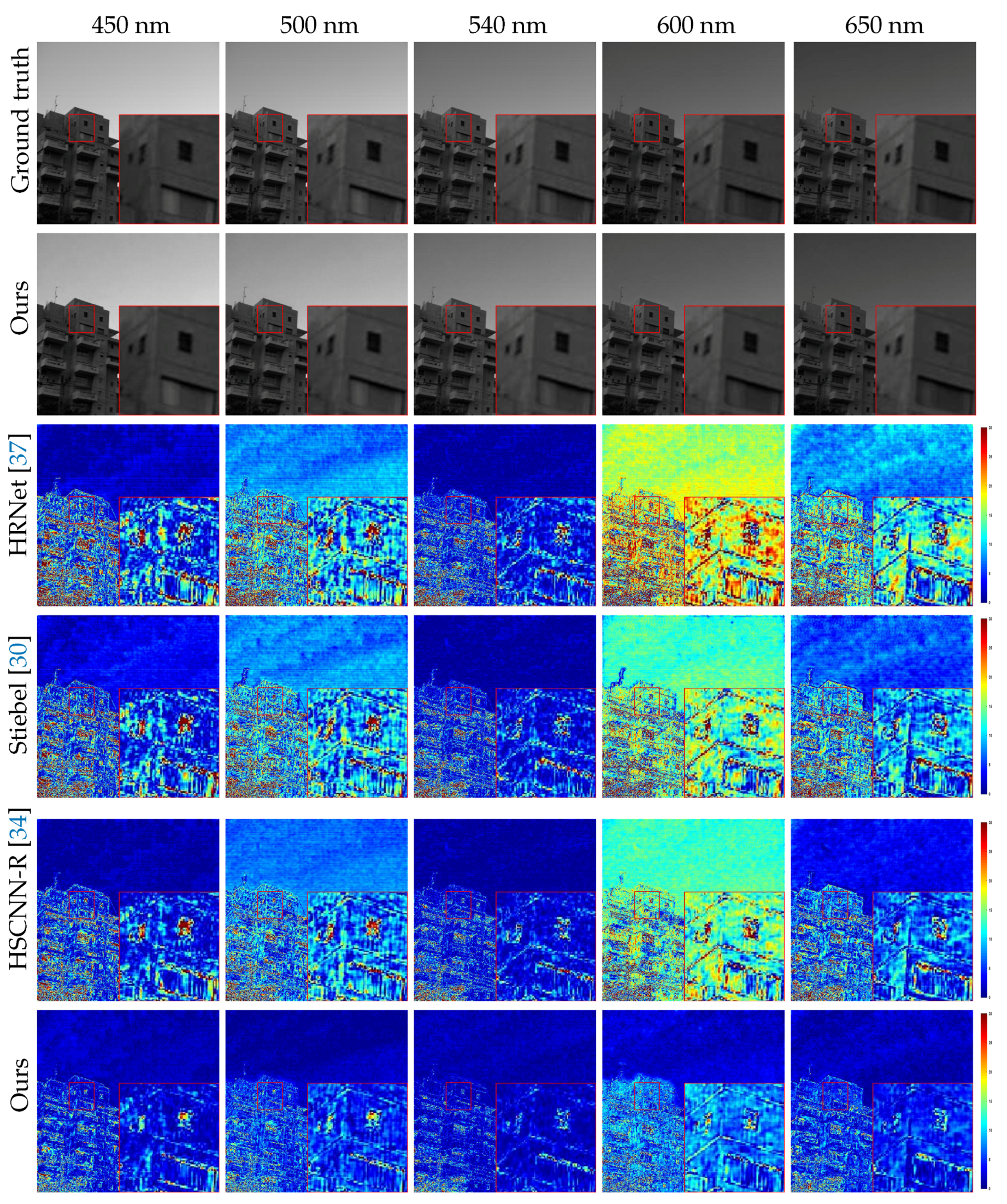
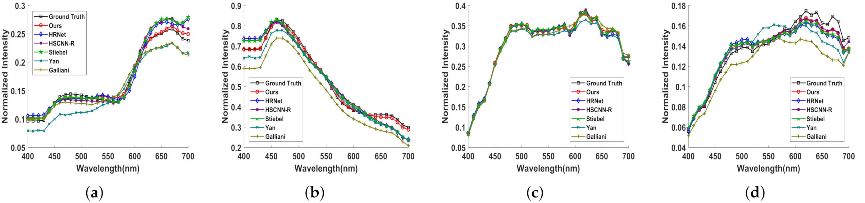
4.2. Results of SR and Analysis

In this study, we compare the proposed RA²UN against 6 existing methods including Arad [17], Galliani [23], Yan [26], Stiebel [30], HSCNN-R [34] and HRNet [37]. Among them, the Arad is an early SR approach based on sparse recovery, while the others are based on CNNs. For a fair comparison, all models retrain on the final training set, save on the final validation set and evaluate on the final testing set for the two tracks of the NTIRE2020 and NTIRE2018 datasets. The quantitative results of final test set of NTIRE2020 and NTIRE2018 “Clean” and “Real World” tracks are listed in

Table 3. The quantitative results of final test set of NTIRE2020 “Clean” and “Real World” tracks. The best and second best results are bold and underlined.

Method	Clean			Real World
	MRAE (↓)	RMSE (↓)	SAM (↓)	MRAE (↓)	RMSE (↓)	SAM (↓)
Ours	0.03446	0.01158	2.39933	0.06554	0.01712	3.35699
Stiebel [30]	0.04008	0.01518	2.73916	0.07141	0.01912	3.68491
HSCNN-R [34]	0.04406	0.01543	2.94031	0.07039	0.01893	3.60987
HRNet [37]	0.04202	0.01575	2.83058	0.07042	0.02035	3.71418
Yan [26]	0.10351	0.02844	4.90422	0.09942	0.03005	4.54294
Galliani [23]	0.07949	0.02788	4.52770	0.10794	0.03307	4.79334
Arad [17]	0.07873	0.03305	5.57166	———	———	———

and

Table 4. The quantitative results of final test set of NTIRE2018 “Clean” and “Real World” tracks. The best and second best results are bold and underlined.

Method	Clean			Real World
	MRAE (↓)	RMSE (↓)	SAM (↓)	MRAE (↓)	RMSE (↓)	SAM (↓)
Ours	0.01141	10.4923	0.80815	0.02868	22.0813	1.52763
HSCNN-R [34]	0.01330	12.8519	0.96004	0.03014	23.5697	1.65147
HRNet [37]	0.01369	13.5165	1.00645	0.02905	22.8282	1.57253
Stiebel [30]	0.01536	15.5253	1.14655	0.03118	24.0600	1.70200
Yan [26]	0.03036	24.2971	1.67274	0.04576	31.8332	2.18224
Galliani [23]	0.05130	37.6802	1.77410	0.07749	49.2496	2.32531
Arad [17]	0.08094	59.4085	5.02125	———	———	———

. Since the camera response function is unknown, Arad is only suitable for measuring on “Clean” tracks. It can be seen that our RA²UN performs the best results under MRAE, RMSE and SAM metrics on all the tracks. As for the ranking metrics MRAE, the proposed method achieves relative reduction of $14.02\%$, $6.89\%$, $14.21\%$ and $1.27\%$ over the second best results on corresponding established datasets. In addition, we can obtain the smallest SAM values, which indicate that our reconstructed HSIs contain better spectral quality.

Also, we show the visual comparison of the five selected bands on different example images of the final test set in Figure 5, Figure 6, Figure 7 and Figure 8. The ground truth, our results and error images are displayed from top to bottom. The error images are the heat maps of MRAE between the ground truth and the recovered HSI. The bluer the displayed color, the better the reconstructed spectrum. As can be seen, our approach yields better recovery results and have less reconstruction error than other competitors. Besides, the spectral response curves of four selected spatial points are painted in Figure 9. The red line is our result and the black one denotes the groundtruth spectrum. The rest are the results of the comparison methods. Obviously, the reconstructed results of RA²UN are much closer to the groundtruth spectrum than the others.

5. Conclusions

In this paper, we propose a novel RA²UN network for SR. Concretely, the backbone of RA²UN network consists of several DIRB blocks instead of paired plain convolutional units. To boost the spatial feature representations, a trainable SAA module is developed to highlight the features in the important regions selectively. Furthermore, we present a novel CAA module to adaptively recalibrate channel-wise feature responses by exploiting first-order statistics and second-order ones for enhance learning capacity of the network. To find a better solution, an additional boundary-aware constraint is built to guide network to learn salient information in edge localization and recover more accurate details. Extensive experiments on challenging benchmarks demonstrate the superiority of our RA²UN network in terms of numerical and visual measurements.

References

1. Chang, C.I. Hyperspectral Data Exploitation: Theory and Applications; John Wiley & Sons: Hoboken, NJ, USA, 2007. [Google Scholar]
2. Uzair, M.; Mahmood, A.; Mian, A. Hyperspectral face recognition with spatiospectral information fusion and PLS regression. IEEE Trans. Image Process. 2015, 24, 1127–1137. [Google Scholar] [CrossRef]
3. Li, J.; Xi, B.; Du, Q.; Song, R.; Li, Y.; Ren, G. Deep Kernel Extreme-Learning Machine for the Spectral–Spatial Classification of Hyperspectral Imagery. Remote Sens. 2018, 10, 2036. [Google Scholar] [CrossRef] [Green Version]
4. Li, J.; Du, Q.; Li, Y.; Li, W. Hyperspectral image classification with imbalanced data based on orthogonal complement subspace projection. IEEE Trans. Geosci. Remote Sens. 2018, 56, 3838–3851. [Google Scholar] [CrossRef]
5. Tochon, G.; Chanussot, J.; Dalla Mura, M.; Bertozzi, A.L. Object tracking by hierarchical decomposition of hyperspectral video sequences: Application to chemical gas plume tracking. IEEE Trans. Geosci. Remote Sens. 2017, 55, 4567–4585. [Google Scholar] [CrossRef]
6. Green, R.O.; Eastwood, M.L.; Sarture, C.M.; Chrien, T.G.; Aronsson, M.; Chippendale, B.J.; Faust, J.A.; Pavri, B.E.; Chovit, C.J.; Solis, M.; et al. Imaging spectroscopy and the airborne visible/infrared imaging spectrometer (AVIRIS). Remote Sens. Environ. 1998, 65, 227–248. [Google Scholar] [CrossRef]
7. James, J. Spectrograph Design Fundamentals; Cambridge University Press: Cambridge, UK, 2007. [Google Scholar]
8. Schechner, Y.Y.; Nayar, S.K. Generalized mosaicing: Wide field of view multispectral imaging. IEEE Trans. Pattern Anal. Mach. Intell. 2002, 24, 1334–1348. [Google Scholar] [CrossRef] [Green Version]
9. Wagadarikar, A.; John, R.; Willett, R.; Brady, D. Single disperser design for coded aperture snapshot spectral imaging. Appl. Opt. 2008, 47, B44–B51. [Google Scholar] [CrossRef] [PubMed] [Green Version]
10. Tanriverdi, F.; Schuldt, D.; Thiem, J. Dual snapshot hyperspectral imaging system for 41-band spectral analysis and stereo reconstruction. In Proceedings of the International Symposium on Visual Computing, Lake Tahoe, NV, USA, 7–9 October 2019; pp. 3–13. [Google Scholar]
11. Beletkaia, E.; Pozo, J. More Than Meets the Eye: Applications enabled by the non-stop development of hyperspectral imaging technology. PhotonicsViews 2020, 17, 24–26. [Google Scholar] [CrossRef]
12. Descour, M.; Dereniak, E. Computed-tomography imaging spectrometer: Experimental calibration and reconstruction results. Appl. Opt. 1995, 34, 4817–4826. [Google Scholar] [CrossRef] [PubMed]
13. Vandervlugt, C.; Masterson, H.; Hagen, N.; Dereniak, E.L. Reconfigurable liquid crystal dispersing element for a computed tomography imaging spectrometer. In Algorithms and Technologies for Multispectral, Hyperspectral, and Ultraspectral Imagery XIII; International Society for Optics and Photonics: Bellingham, WA, USA, 2007; Volume 6565. [Google Scholar]
14. Wagadarikar, A.A.; Pitsianis, N.P.; Sun, X.; Brady, D.J. Video rate spectral imaging using a coded aperture snapshot spectral imager. Opt. Express 2009, 17, 6368–6388. [Google Scholar] [CrossRef] [PubMed]
15. Nguyen, R.M.; Prasad, D.K.; Brown, M.S. Training-based spectral reconstruction from a single RGB image. In Proceedings of the European Conference on Computer Vision, Zurich, Switzerland, 6–12 September 2014; pp. 186–201. [Google Scholar]
16. Robles-Kelly, A. Single image spectral reconstruction for multimedia applications. In Proceedings of the 23rd ACM international conference on Multimedia, Brisbane, QLD, Australia, 26–30 October 2015; pp. 251–260. [Google Scholar]
17. Arad, B.; Ben-Shahar, O. Sparse recovery of hyperspectral signal from natural RGB images. In Proceedings of the European Conference on Computer Vision, Amsterdam, The Netherlands, 8–16 October 2016; pp. 19–34. [Google Scholar]
18. Jia, Y.; Zheng, Y.; Gu, L.; Subpa-Asa, A.; Lam, A.; Sato, Y.; Sato, I. From RGB to spectrum for natural scenes via manifold-based mapping. In Proceedings of the IEEE International Conference on Computer Vision, Venice, Italy, 22–29 October 2017; pp. 4705–4713. [Google Scholar]
19. Aeschbacher, J.; Wu, J.; Timofte, R. In defense of shallow learned spectral reconstruction from RGB images. In Proceedings of the IEEE International Conference on Computer Vision, Venice, Italy, 22–29 October 2017; pp. 471–479. [Google Scholar]
20. Zhang, S.; Wang, L.; Fu, Y.; Zhong, X.; Huang, H. Computational Hyperspectral Imaging Based on Dimension-Discriminative Low-Rank Tensor Recovery. In Proceedings of the IEEE/CVF International Conference on Computer Vision (ICCV), Seoul, Korea, 27–28 October 2019. [Google Scholar]
21. Li, J.; Cui, R.; Li, B.; Song, R.; Li, Y.; Dai, Y.; Du, Q. Hyperspectral Image Super-Resolution by Band Attention Through Adversarial Learning. IEEE Trans. Geosci. Remote Sens. 2020, 58, 4304–4318. [Google Scholar] [CrossRef]
22. Li, J.; Cui, R.; Li, B.; Song, R.; Li, Y.; Du, Q. Hyperspectral Image Super-Resolution with 1D–2D Attentional Convolutional Neural Network. Remote Sens. 2019, 11, 2859. [Google Scholar] [CrossRef] [Green Version]
23. Galliani, S.; Lanaras, C.; Marmanis, D.; Baltsavias, E.; Schindler, K. Learned spectral super-resolution. arXiv 2017, arXiv:1703.09470. [Google Scholar]
24. Rangnekar, A.; Mokashi, N.; Ientilucci, E.; Kanan, C.; Hoffman, M. Aerial spectral super-resolution using conditional adversarial networks. arXiv 2017, arXiv:1712.08690. [Google Scholar]
25. Xiong, Z.; Shi, Z.; Li, H.; Wang, L.; Liu, D.; Wu, F. Hscnn: Cnn-based hyperspectral image recovery from spectrally undersampled projections. In Proceedings of the IEEE International Conference on Computer Vision, Venice, Italy, 22–29 October 2017; pp. 518–525. [Google Scholar]
26. Yan, Y.; Zhang, L.; Li, J.; Wei, W.; Zhang, Y. Accurate spectral super-resolution from single RGB image using multi-scale CNN. In Proceedings of the Chinese Conference on Pattern Recognition and Computer Vision (PRCV), Guangzhou, China, 23–26 November 2018; pp. 206–217. [Google Scholar]
27. Fu, Y.; Zhang, T.; Zheng, Y.; Zhang, D.; Huang, H. Joint Camera Spectral Sensitivity Selection and Hyperspectral Image Recovery. In Proceedings of the European Conference on Computer Vision (ECCV), Munich, Germany, 8–14 September 2018; pp. 788–804. [Google Scholar]
28. Nie, S.; Gu, L.; Zheng, Y.; Lam, A.; Ono, N.; Sato, I. Deeply Learned Filter Response Functions for Hyperspectral Reconstruction. In Proceedings of the IEEE Conference on Computer Vision and Pattern Recognition, Salt Lake City, UT, USA, 18–22 June 2018; pp. 4767–4776. [Google Scholar]
29. Arad, B.; Ben-Shahar, O.; Timofte, R. Ntire 2018 challenge on spectral reconstruction from RGB images. In Proceedings of the IEEE Conference on Computer Vision and Pattern Recognition Workshops, Salt Lake City, UT, USA, 18–22 June 2018; pp. 929–938. [Google Scholar]
30. Stiebel, T.; Koppers, S.; Seltsam, P.; Merhof, D. Reconstructing spectral images from RGB-images using a convolutional neural network. In Proceedings of the IEEE Conference on Computer Vision and Pattern Recognition Workshops, Salt Lake City, UT, USA, 18–22 June 2018; pp. 948–953. [Google Scholar]
31. Can, Y.B.; Timofte, R. An efficient CNN for spectral reconstruction from RGB images. arXiv 2018, arXiv:1804.04647. [Google Scholar]
32. Alvarez-Gila, A.; van de Weijer, J.; Garrote, E. Adversarial networks for spatial context-aware spectral image reconstruction from RGB. In Proceedings of the IEEE International Conference on Computer Vision, Venice, Italy, 22–29 October 2017; pp. 480–490. [Google Scholar]
33. Koundinya, S.; Sharma, H.; Sharma, M.; Upadhyay, A.; Manekar, R.; Mukhopadhyay, R.; Karmakar, A.; Chaudhury, S. 2D–3D cnn based architectures for spectral reconstruction from RGB images. In Proceedings of the IEEE Conference on Computer Vision and Pattern Recognition Workshops, Salt Lake City, UT, USA, 18–22 June 2018; pp. 844–851. [Google Scholar]
34. Shi, Z.; Chen, C.; Xiong, Z.; Liu, D.; Wu, F. Hscnn+: Advanced cnn-based hyperspectral recovery from RGB images. In Proceedings of the IEEE Conference on Computer Vision and Pattern Recognition Workshops, Salt Lake City, UT, USA, 18–22 June 2018; pp. 939–947. [Google Scholar]
35. Arad, B.; Timofte, R.; Ben-Shahar, O.; Lin, Y.T.; Finlayson, G.D. Ntire 2020 challenge on spectral reconstruction from an RGB image. In Proceedings of the IEEE/CVF Conference on Computer Vision and Pattern Recognition Workshops, Seattle, WA, USA, 14–19 June 2020; pp. 446–447. [Google Scholar]
36. Li, J.; Wu, C.; Song, R.; Li, Y.; Liu, F. Adaptive weighted attention network with camera spectral sensitivity prior for spectral reconstruction from RGB images. In Proceedings of the IEEE/CVF Conference on Computer Vision and Pattern Recognition Workshops, Seattle, WA, USA, 14–19 June 2020; pp. 462–463. [Google Scholar]
37. Zhao, Y.; Po, L.M.; Yan, Q.; Liu, W.; Lin, T. Hierarchical regression network for spectral reconstruction from RGB images. In Proceedings of the IEEE/CVF Conference on Computer Vision and Pattern Recognition Workshops, Seattle, WA, USA, 14–19 June 2020; pp. 422–423. [Google Scholar]
38. Peng, H.; Chen, X.; Zhao, J. Residual pixel attention network for spectral reconstruction from RGB images. In Proceedings of the IEEE/CVF Conference on Computer Vision and Pattern Recognition Workshops, Seattle, WA, USA, 14–19 June 2020; pp. 486–487. [Google Scholar]
39. Joslyn Fubara, B.; Sedky, M.; Dyke, D. RGB to Spectral Reconstruction via Learned Basis Functions and Weights. In Proceedings of the IEEE/CVF Conference on Computer Vision and Pattern Recognition Workshops, Seattle, WA, USA, 14–19 June 2020; pp. 480–481. [Google Scholar]
40. Banerjee, A.; Palrecha, A. MXR-U-Nets for Real Time Hyperspectral Reconstruction. arXiv 2020, arXiv:2004.07003. [Google Scholar]
41. Nathan, D.S.; Uma, K.; Vinothini, D.S.; Bama, B.S.; Roomi, S. Light Weight Residual Dense Attention Net for Spectral Reconstruction from RGB Images. arXiv 2020, arXiv:2004.06930. [Google Scholar]
42. Kaya, B.; Can, Y.B.; Timofte, R. Towards spectral estimation from a single RGB image in the wild. In Proceedings of the 2019 IEEE/CVF International Conference on Computer Vision Workshop (ICCVW), Seoul, Korea, 27–28 October 2019; pp. 3546–3555. [Google Scholar]
43. Zhang, L.; Lang, Z.; Wang, P.; Wei, W.; Liao, S.; Shao, L.; Zhang, Y. Pixel-Aware Deep Function-Mixture Network for Spectral Super-Resolution. In Proceedings of the AAAI, New York, NY, USA, 7–12 February 2020; pp. 12821–12828. [Google Scholar]
44. Hang, R.; Li, Z.; Liu, Q.; Bhattacharyya, S.S. Prinet: A Prior Driven Spectral Super-Resolution Network. In Proceedings of the 2020 IEEE International Conference on Multimedia and Expo (ICME), London, UK, 6–10 July 2020; pp. 1–6. [Google Scholar]
45. Li, J.; Wu, C.; Song, R.; Xie, W.; Ge, C.; Li, B.; Li, Y. Hybrid 2-D-3-D Deep Residual Attentional Network With Structure Tensor Constraints for Spectral Super-Resolution of RGB Images. IEEE Trans. Geosci. Remote Sens. 2020, 1–15. [Google Scholar] [CrossRef]
46. Chen, L.; Zhang, H.; Xiao, J.; Nie, L.; Shao, J.; Liu, W.; Chua, T.S. SCA-CNN: Spatial and Channel-Wise Attention in Convolutional Networks for Image Captioning. In Proceedings of the IEEE Conference on Computer Vision and Pattern Recognition (CVPR), Honolulu, HI, USA, 21–26 July 2017. [Google Scholar]
47. Hu, J.; Shen, L.; Sun, G. Squeeze-and-excitation networks. In Proceedings of the IEEE Conference on Computer Vision and Pattern Recognition Workshops, Salt Lake City, UT, USA, 18–22 June 2018; pp. 7132–7141. [Google Scholar]
48. Wang, X.; Girshick, R.; Gupta, A.; He, K. Non-local neural networks. In Proceedings of the IEEE Conference on Computer Vision and Pattern Recognition Workshops, Salt Lake City, UT, USA, 18–22 June 2018; pp. 7794–7803. [Google Scholar]
49. Zhang, Y.; Li, K.; Li, K.; Wang, L.; Zhong, B.; Fu, Y. Image super-resolution using very deep residual channel attention networks. In Proceedings of the European Conference on Computer Vision (ECCV), Munich, Germany, 8–14 September 2018; pp. 286–301. [Google Scholar]
50. Dai, T.; Cai, J.; Zhang, Y.; Xia, S.T.; Zhang, L. Second-order attention network for single image super-resolution. In Proceedings of the IEEE Conference On Computer Vision And Pattern Recognition, Long Beach, CA, USA, 15–20 June 2019; pp. 11065–11074. [Google Scholar]
51. Dai, T.; Zha, H.; Jiang, Y.; Xia, S.T. Image Super-Resolution via Residual Block Attention Networks. In Proceedings of the IEEE International Conference on Computer Vision Workshops, Seoul, Korea, 27–28 October 2019. [Google Scholar]
52. Xia, B.N.; Gong, Y.; Zhang, Y.; Poellabauer, C. Second-order non-local attention networks for person re-identification. In Proceedings of the IEEE International Conference on Computer Vision Workshops, Seoul, Korea, 27–28 October 2019; pp. 3760–3769. [Google Scholar]
53. Zhang, Z.; Lan, C.; Zeng, W.; Jin, X.; Chen, Z. Relation-Aware Global Attention for Person Re-identification. In Proceedings of the IEEE/CVF Conference on Computer Vision and Pattern Recognition, Seattle, WA, USA, 14–19 June 2020; pp. 3186–3195. [Google Scholar]
54. Zuniga, O.A.; Haralick, R.M. Integrated directional derivative gradient operator. IEEE Trans. Syst. Man, Cybern. 1987, 17, 508–517. [Google Scholar] [CrossRef]
55. Kingma, D.P.; Ba, J. Adam: A method for stochastic optimization. arXiv 2014, arXiv:1412.6980. [Google Scholar]
Figure 1. Network architecture of the proposed RA2UN network. The input of the RA2UN network is RGB images and the output is the corresponding reconstructed HSIs. The detailed network and parameters setting can be referenced from Table 1.
Remotesensing 13 00115 g001
Figure 2. The overview of spatial augmented attention module. ⊕ denotes the element-wise summation.
Remotesensing 13 00115 g002
Figure 3. The overview of channel augmented attention module. ⊕ denotes the element-wise summation.
Remotesensing 13 00115 g003
Figure 4. The first row (ad) shows several original images from the NTIRE2020 dataset. The second row (eh) displays the effect of edge extraction and the white lines represent boundary information.
Remotesensing 13 00115 g004
Figure 5. Visual comparison of the five selected bands on “ARAD_HS_0455” image from the final testing set of NTIRE2020 “Clean” track. The best view on the screen.
Remotesensing 13 00115 g005
Figure 6. Visual comparison of the five selected bands on “ARAD_HS_0451” image from the final testing set of NTIRE2020 “Real World” track. The best view on the screen.
Remotesensing 13 00115 g006
Figure 7. Visual comparison of the five selected bands on “BGU_HS_00265” image from the final testing set of NTIRE2018 “Clean” track. The best view on the screen.
Remotesensing 13 00115 g007
Figure 8. Visual comparison of the five selected bands on “BGU_HS_00259” image from the final testing set of NTIRE2018 “Real World” track. The best view on the screen.
Remotesensing 13 00115 g008
Figure 9. Spectral response curves of selected several spatial points from the reconstructed HSIs. (a,b) are for the NTIRE2020 “Clean” and “Real World” tracks respectively. (c,d) are for the NTIRE2018 “Clean” and “Real World” track respectively.
Remotesensing 13 00115 g009