
Flood Hazard Mapping Using Fuzzy Logic, Analytical Hierarchy Process, and Multi-Source Geospatial Datasets


Abstract
:1. Introduction
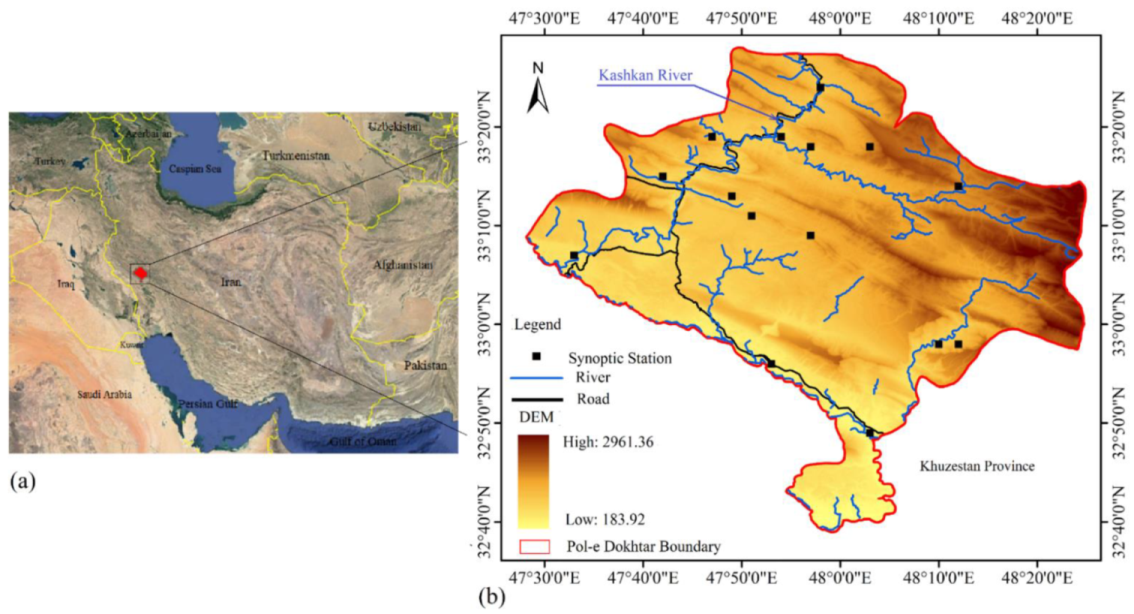
2. Study Area and Case Study
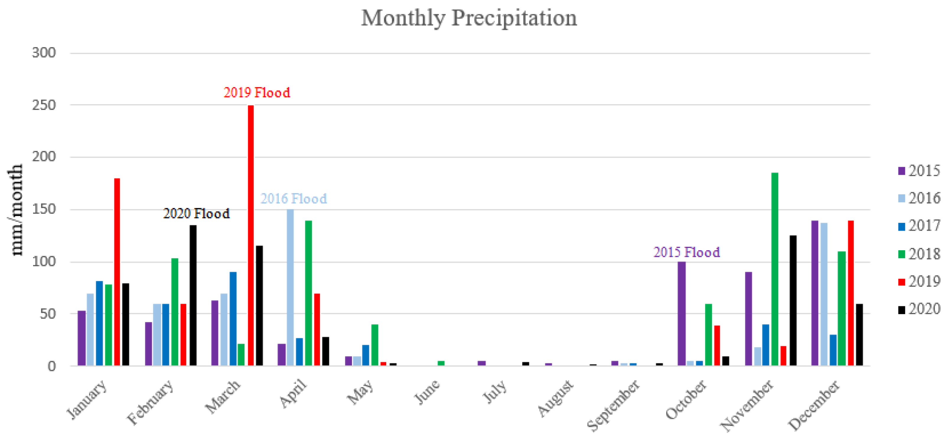
Flooded Areas and Rainfall History
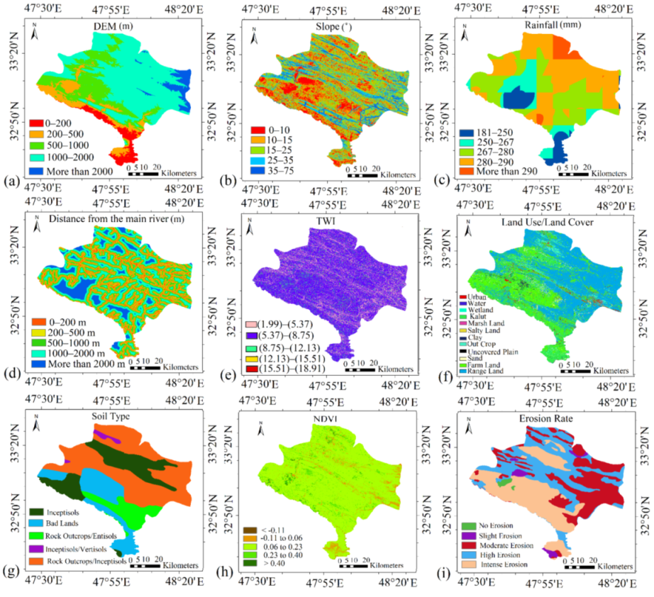
3. Datasets
3.1. Digital Elevation Model (DEM)
3.2. Slope
3.3. Rainfall
3.4. Distance from the Main Rivers
3.5. Topographic Wetness Index (TWI)
3.6. Land Use/Land Cover (LULC)
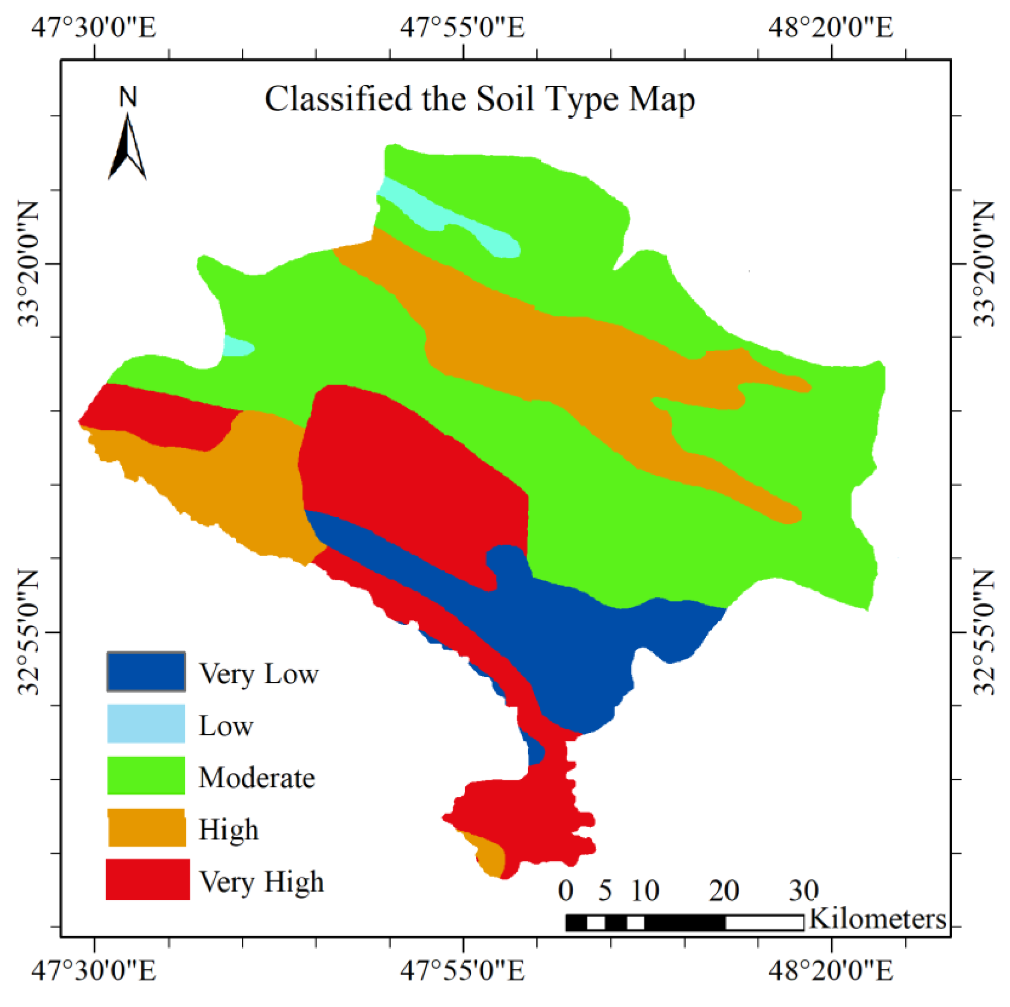
3.7. Soil Type
3.8. Normalized Difference Vegetation Index (NDVI)
3.9. Erosion Rate
3.10. Sentinel-1 Images
4. Methodology
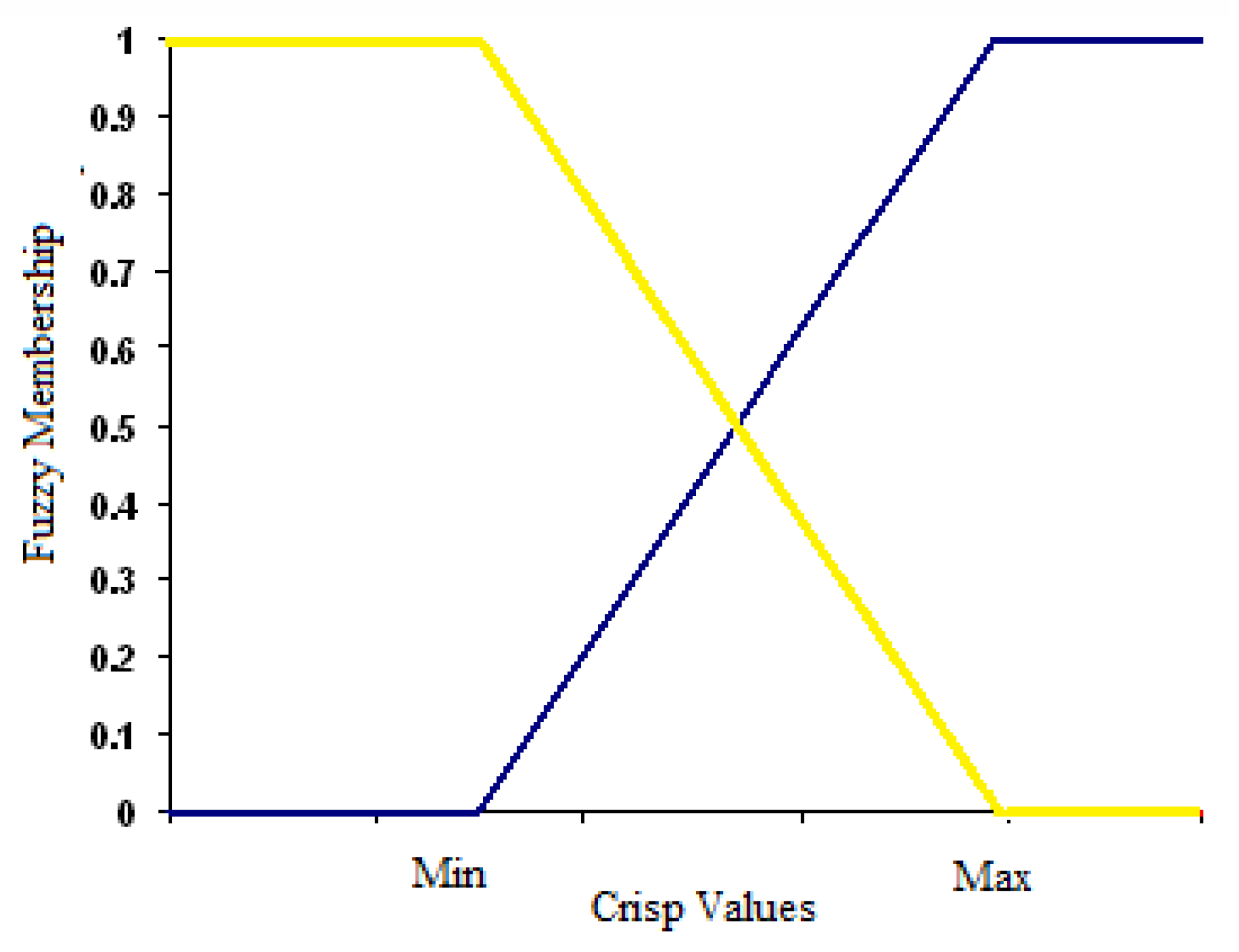
4.1. Fuzzification
4.2. Analytic Hierarchy Process (AHP)
4.3. Fuzzy Overlay
4.4. Jenks Natural Breaks Classification
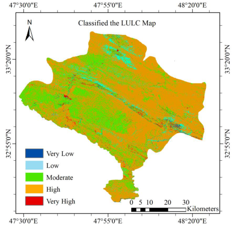
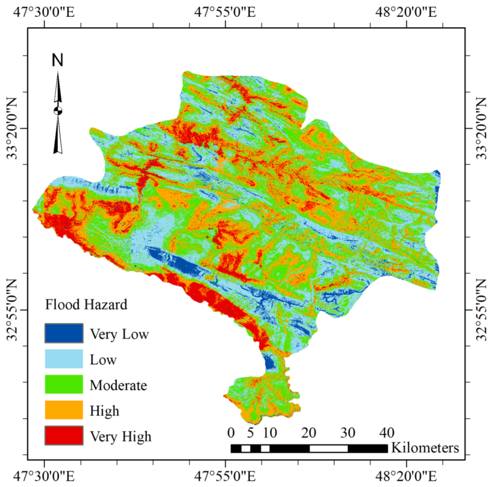
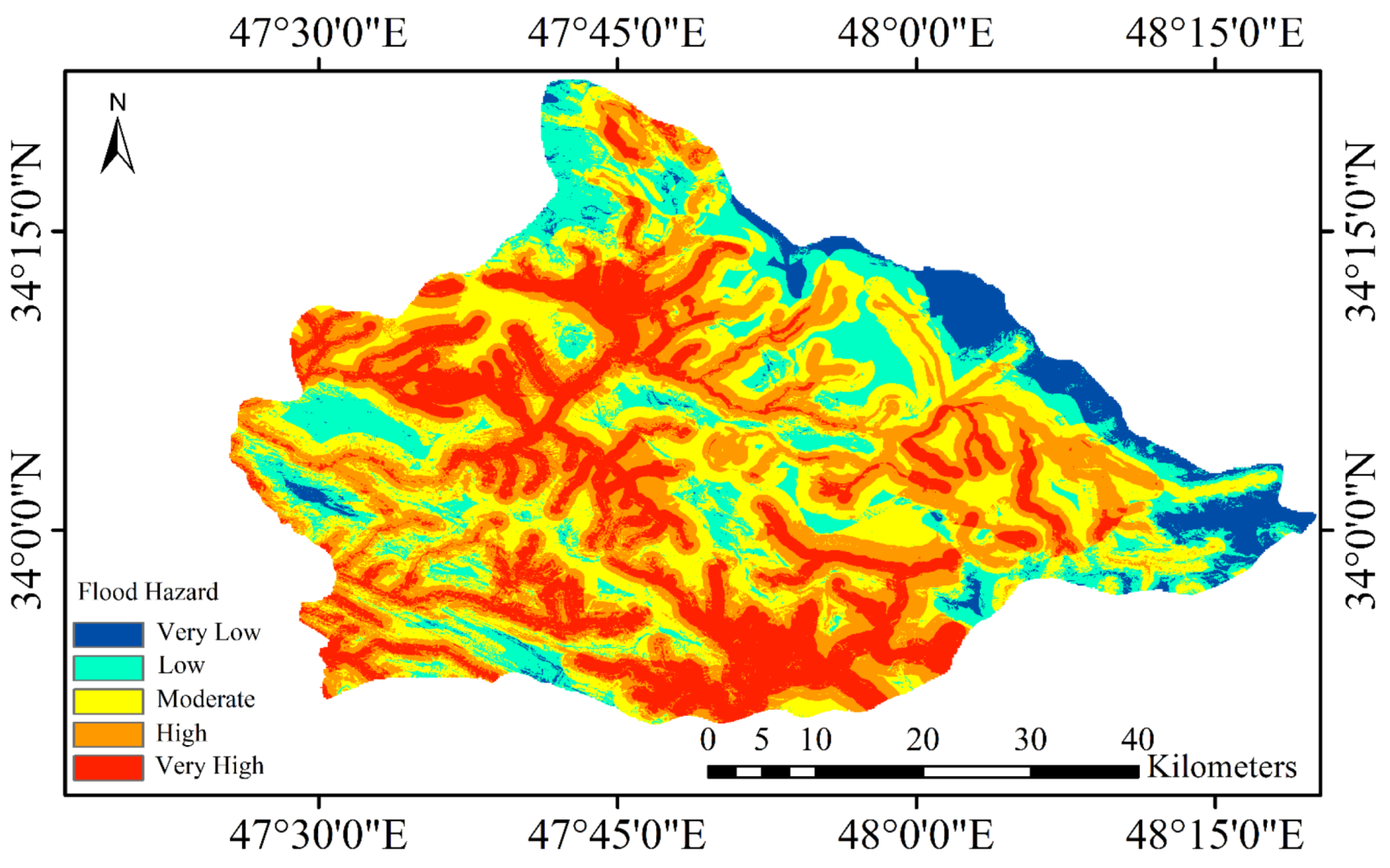
4.5. Final Flood Hazard Map
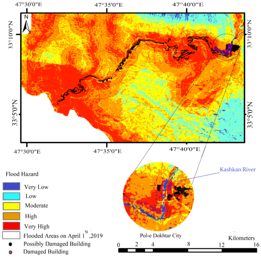
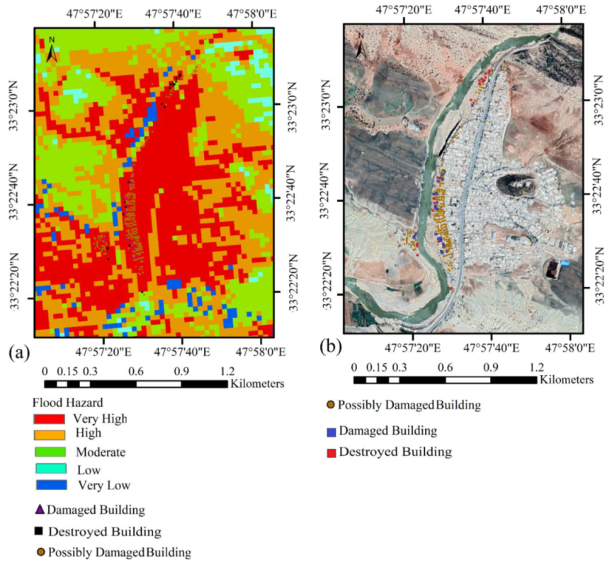
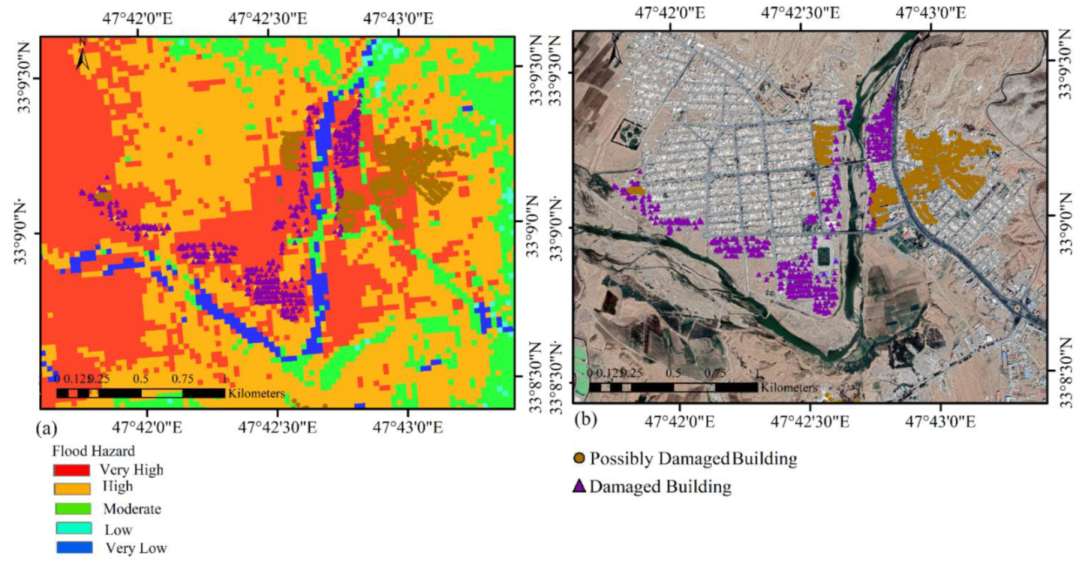
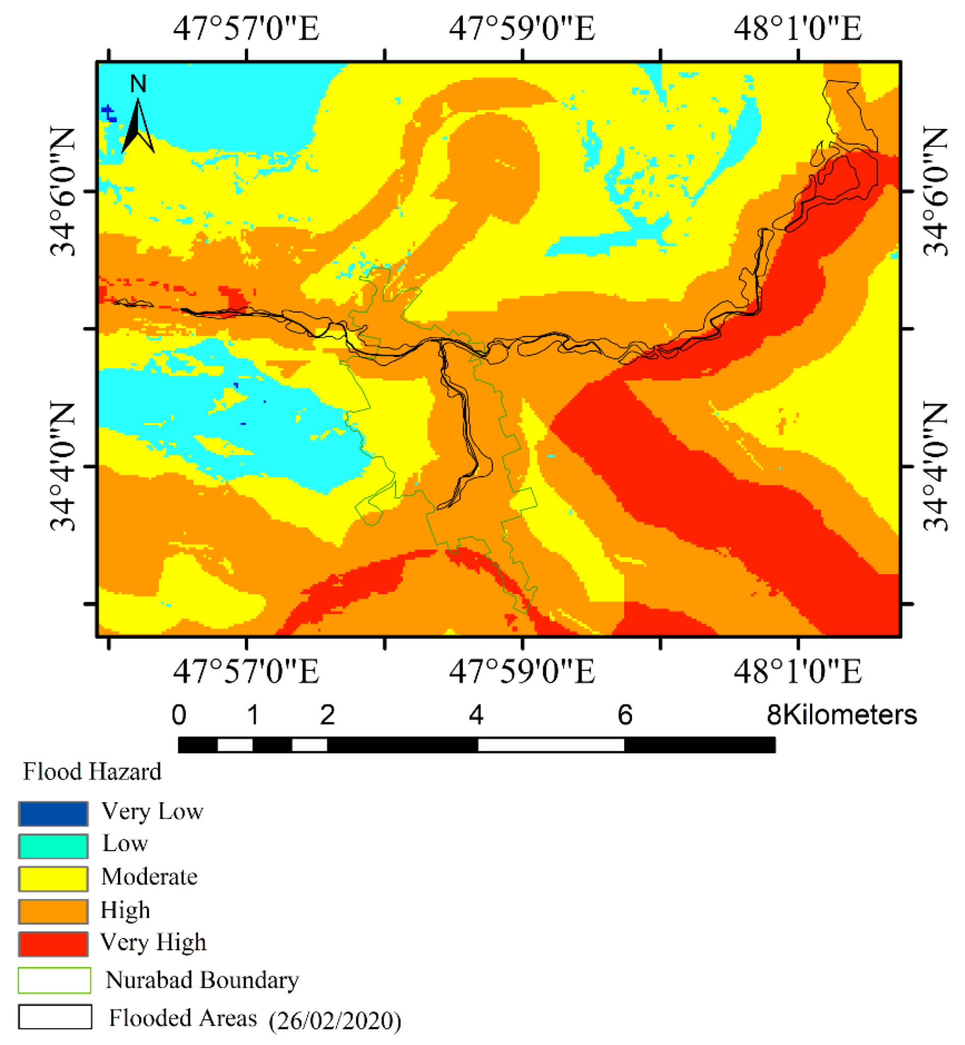
4.6. Validation
5. Results
6. Discussion
7. Conclusions
Author Contributions
Funding
Institutional Review Board Statement
Informed Consent Statement
Data Availability Statement
Conflicts of Interest
References
- Adjei-Darko, P. Remote Sensing and Geographic Information Systems for Flood Risk Mapping and Near Real-time Flooding Extent Assessment in the Greater Accra Metropolitan Area. Master’s Thesis, KTH, Stockholm, Sweden, 2017; pp. 1–74. [Google Scholar]
- Marchand, M.; Buurman, J.; Pribadi, A.; Kurniawan, A. Damage and casualties modelling as part of a vulnerability assessment for tsunami hazards: A case study from Aceh, Indonesia. J. Flood Risk Manag. 2009, 2, 120–131. [Google Scholar] [CrossRef]
- Taylor, J.; Lai, K.M.; Davies, M.; Clifton, D.; Ridley, I.; Biddulph, P. Flood management: Prediction of microbial contamination in large-scale floods in urban environments. Environ. Int. 2011, 37, 1019–1029. [Google Scholar] [CrossRef] [PubMed]
- Dawod, G.M.; Mirza, M.N.; Al-Ghamdi, K.A. GIS-based estimation of flood hazard impacts on road network in Makkah city, Saudi Arabia. Environ. Earth Sci. 2012, 67, 2205–2215. [Google Scholar] [CrossRef]
- Heidari, A. Flood vulnerability of the Karun River System and short-term mitigation measures. J. Flood Risk Manag. 2013, 7, 65–80. [Google Scholar] [CrossRef]
- Rahmati, O.; Zeinivand, H.; Besharat, M. Flood hazard zoning in Yasooj region, Iran, using GIS and multi-criteria decision analysis. Geom. Nat. Hazards Risk 2015, 7, 1000–1017. [Google Scholar] [CrossRef] [Green Version]
- Blöschl, G.; Gaál, L.; Hall, J.; Kiss, A.; Komma, J.; Nester, T.; Parajka, J.; Perdigão, R.A.P.; Plavcová, L.; Rogger, M.; et al. Increasing river floods: Fiction or reality? Wiley Interdiscip. Rev. Water 2015, 2, 329–344. [Google Scholar] [CrossRef]
- Nones, M.; Pescaroli, G. Implications of cascading effects for the EU Floods Directive. Int. J. River Basin Manag. 2015, 14, 195–204. [Google Scholar] [CrossRef]
- Tellman, B.; Sullivan, J.A.; Kuhn, C.; Kettner, A.J.; Doyle, C.S.; Brakenridge, G.R.; Erickson, T.A.; Slayback, D.A. Satellite imaging reveals increased proportion of population exposed to floods. Nature 2021, 596, 80–86. [Google Scholar] [CrossRef]
- Aggarwal, S.P.; Expressway, J.; State, J.P.; Division, W.R.; Road, K. Flood Inundation Hazard Modelling of the River Kaduna Using Remote Sensing and Geographic Information Systems. J. Appl. Sci. Res. 2008, 4, 1822–1833. [Google Scholar]
- El Morjani, Z.E.A.; Ennasr, M.S.; Elmouden, A.; Idbraim, S.; Bouaakaz, B.; Saad, A. Flood Hazard Mapping and Modeling Using GIS Applied to the Souss River Watershed. In The Souss-Massa River Basin, Morocco; Springer: Cham, Switzerland, 2016; pp. 57–93. [Google Scholar] [CrossRef]
- Toriman, M.E.; Gazim, M.B.; Mokhtar, M.; SA, S.M.; Jaafar, O.; Karim, O.; Aziz, N.A.A. Integration of 1-d Hydrodynamic Model and GIS Approach in Flood Management Study in Malaysia. Res. J. Earth Sci. 2009, 1, 22–27. [Google Scholar]
- Government of the Islamic Republic of Iran/UN Country Team in Iran. Post Disaster Needs Assessment (PDNA): Iran 2019 Floods in Lorestan, Khuzestan and Golestan Provinces; Government of Iran: Tehran, Iran, 2019.
- Díez-Herrero, A.; Huerta, L.L.; Isidro, M.L. A Handbook on Flood Hazard Mapping Methodologies; Geological Survey of Spain: Madrid, Spain, 2013; ISBN 9788478408139. [Google Scholar]
- Sami, G.; Abdelwahhab, F.; Yahyaoui, H.; Abdelghani, F. Flood hazard in the city of chemora (algeria). An. Univ. Din Oradea Ser. Geogr. 2021, 31, 22–27. [Google Scholar] [CrossRef]
- Schumann, G.J.-P.; Brakenridge, G.R.; Kettner, A.J.; Kashif, R.; Niebuhr, E. Assisting Flood Disaster Response with Earth Observation Data and Products: A Critical Assessment. Remote Sens. 2018, 10, 1230. [Google Scholar] [CrossRef] [Green Version]
- Jha, A.K.; Bloch, R.; Lamond, J. Cities and Flooding: A Guide to Integrated Urban Flood Risk Management for the 21st Century; World Bank Publications: Washington, DC, USA, 2012; ISBN 9780821388662. [Google Scholar]
- Yan, K.; Di Baldassarre, G.; Solomatine, D.P.; Schumann, G. A review of low-cost space-borne data for flood modelling: Topography, flood extent and water level. Hydrol. Process. 2015, 29, 3368–3387. [Google Scholar] [CrossRef]
- Mahdavi, S.; Salehi, B.; Huang, W.; Amani, M.; Brisco, B. A PolSAR Change Detection Index Based on Neighborhood Information for Flood Mapping. Remote Sens. 2019, 11, 1854. [Google Scholar] [CrossRef] [Green Version]
- The European Space Agency. Available online: Https://www.esa.int/Applications/Observing_the_Earth/Copernicus/The_Sentinel_missions (accessed on 26 June 2021).
- Samanta, S.; Pal, D.K.; Palsamanta, B. Flood susceptibility analysis through remote sensing, GIS and frequency ratio model. Appl. Water Sci. 2018, 8, 66. [Google Scholar] [CrossRef] [Green Version]
- Argaz, A.; Ouahman, B.; Darkaoui, A.; Bikhtar, H.; Ayouch, E.; Lazaar, R. Flood Hazard Mapping Using remote sensing and GIS Tools: A case study of Souss Watershed. J. Mater. Environ. Sci. 2019, 10, 170–181. [Google Scholar]
- Bandi, A.S.; Meshapam, S.; Deva, P. A geospatial approach to flash flood hazard mapping in the city of Warangal, Telangana, India. Environ. Socio-Econ. Stud. 2019, 7, 1–13. [Google Scholar] [CrossRef] [Green Version]
- Ullah, K.; Zhang, J. GIS-based flood hazard mapping using relative frequency ratio method: A case study of Panjkora River Basin, eastern Hindu Kush, Pakistan. PLoS ONE 2020, 15, e0229153. [Google Scholar] [CrossRef] [Green Version]
- Amani, M.; Salehi, B.; Mahdavi, S.; Masjedi, A.; Dehnavi, S. Temperature-Vegetation-soil Moisture Dryness Index (TVMDI). Remote Sens. Environ. 2017, 197, 1–14. [Google Scholar] [CrossRef]
- Yadollahie, M. The Flood in Iran: A Consequence of the Global Warming? Int. J. Occup. Environ. Med. 2019, 10, 54–56. [Google Scholar] [CrossRef] [Green Version]
- Bui, D.T.; Khosravi, K.; Shahabi, H.; Daggupati, P.; Adamowski, J.F.; Melesse, A.M.; Pham, B.T.; Pourghasemi, H.R.; Mahmoudi, M.; Bahrami, S.; et al. Flood Spatial Modeling in Northern Iran Using Remote Sensing and GIS: A Comparison between Evidential Belief Functions and Its Ensemble with a Multivariate Logistic Regression Model. Remote Sens. 2019, 11, 1589. [Google Scholar] [CrossRef] [Green Version]
- Darand, M.; Sohrabi, M.M. Identifying drought- and flood-prone areas based on significant changes in daily precipitation over Iran. Nat. Hazards 2017, 90, 1427–1446. [Google Scholar] [CrossRef]
- Vaghefi, S.A.; Keykhai, M.; Jahanbakhshi, F.; Sheikholeslami, J.; Ahmadi, A.; Yang, H.; Abbaspour, K.C. The future of extreme climate in Iran. Sci. Rep. 2019, 9, 1464. [Google Scholar] [CrossRef] [PubMed] [Green Version]
- Seddighi, H.; Seddighi, S. How much the Iranian government spent on disasters in the last 100 years? A critical policy analysis. Cost Eff. Resour. Alloc. 2020, 18, 1–11. [Google Scholar] [CrossRef] [PubMed]
- Zhou, C.; Luo, J.; Yang, C.; Li, B.; Wang, S. Flood Monitoring Using Multi-Temporal AVHRR and RADARSAT Imagery. PE RS Photogramm. Eng. Remote Sens. 2000, 66, 633–638. [Google Scholar]
- Citypopulation. Available online: https://www.citypopulation.de/en/iran/lorestan/1508__pol_e_dokhtar/ (accessed on 20 July 2021).
- Nia, E.S.; Asadollahfardi, G.; Heidarzadeh, N. Study of the environmental flow of rivers, a case study, Kashkan River, Iran. J. Water Supply Res. Technol. 2015, 65, 181–194. [Google Scholar] [CrossRef]
- Ghorbanian, A.; Kakooei, M.; Amani, M.; Mahdavi, S.; Mohammadzadeh, A.; Hasanlou, M. Improved land cover map of Iran using Sentinel imagery within Google Earth Engine and a novel automatic workflow for land cover classification using migrated training samples. ISPRS J. Photogramm. Remote Sens. 2020, 167, 276–288. [Google Scholar] [CrossRef]
- Li, K.; Wu, S.; Dai, E.; Xu, Z. Flood loss analysis and quantitative risk assessment in China. Nat. Hazards 2012, 63, 737–760. [Google Scholar] [CrossRef]
- Nedkov, S.; Burkhard, B. Flood regulating ecosystem services—Mapping supply and demand, in the Etropole municipality, Bulgaria. Ecol. Indic. 2012, 21, 67–79. [Google Scholar] [CrossRef]
- NASA JPL NASA Shuttle Radar Topography Mission Global 1 Arc Second [Data Set]. NASA EOSDIS Land Processes DAAC. 2013. Available online: https://doi.org/10.5067/MEaSUREs/SRTM/SRTMGL1.003 (accessed on 1 November 2021).
- Ouma, Y.O.; Tateishi, R. Urban Flood Vulnerability and Risk Mapping Using Integrated Multi-Parametric AHP and GIS: Methodological Overview and Case Study Assessment. Water 2014, 6, 1515–1545. [Google Scholar] [CrossRef]
- Kay, A.L.; Jones, R.; Reynard, N. RCM rainfall for UK flood frequency estimation. II. Climate change results. J. Hydrol. 2006, 318, 163–172. [Google Scholar] [CrossRef]
- Wang, Y.; Hong, H.; Chen, W.; Li, S.; Panahi, M.; Khosravi, K.; Shirzadi, A.; Shahabi, H.; Panahi, S.; Costache, R. Flood susceptibility mapping in Dingnan County (China) using adaptive neuro-fuzzy inference system with biogeography based optimization and imperialistic competitive algorithm. J. Environ. Manag. 2019, 247, 712–729. [Google Scholar] [CrossRef]
- Wang, J.; Petersen, W.; Wolff, D. Validation of Satellite-Based Precipitation Products from TRMM to GPM. Remote Sens. 2021, 13, 1745. [Google Scholar] [CrossRef]
- Jewell, S.A.; Gaussiat, N. An assessment of kriging-based rain-gauge–radar merging techniques. Q. J. R. Meteorol. Soc. 2015, 141, 2300–2313. [Google Scholar] [CrossRef]
- Jin, B.; Wu, Y.; Miao, B.; Wang, X.L.; Guo, P. Bayesian spatiotemporal modeling for blending in situ observations with satellite precipitation estimates. J. Geophys. Res. Atmos. 2014, 119, 1806–1819. [Google Scholar] [CrossRef]
- Karnieli, A. Application of kriging technique to areal precipitation mapping in Arizona. GeoJournal 1990, 22, 391–398. [Google Scholar] [CrossRef]
- Cecinati, F.; Moreno-Ródenas, A.M.; Rico-Ramirez, M.A.; Veldhuis, M.-C.T.; Langeveld, J.G. Considering Rain Gauge Uncertainty Using Kriging for Uncertain Data. Atmosphere 2018, 9, 446. [Google Scholar] [CrossRef] [Green Version]
- Ly, S.; Charles, C.; Degré, A. Geostatistical interpolation of daily rainfall at catchment scale: The use of several variogram models in the Ourthe and Ambleve catchments, Belgium. Hydrol. Earth Syst. Sci. 2011, 15, 2259–2274. [Google Scholar] [CrossRef] [Green Version]
- Glenn, E.; Morino, K.; Nagler, P.; Murray, R.; Pearlstein, S.; Hultine, K. Roles of saltcedar (Tamarix spp.) and capillary rise in salinizing a non-flooding terrace on a flow-regulated desert river. J. Arid. Environ. 2012, 79, 56–65. [Google Scholar] [CrossRef]
- Peucker, T.K.; Douglas, D.H. Detection of Surface-Specific Points by Local Parallel Processing of Discrete Terrain Elevation Data. Comput. Graph. Image Process. 1975, 4, 375–387. [Google Scholar] [CrossRef]
- Luo, W.; Li, X.; Molloy, I.; Di, L.; Stepinski, T. Web Service for extracting stream networks from DEM data. GeoJournal 2013, 79, 183–193. [Google Scholar] [CrossRef]
- Pourali, S.H.; Arrowsmith, C.; Chrisman, N.; Matkan, A.A.; Mitchell, D. Topography Wetness Index Application in Flood-Risk-Based Land Use Planning. Appl. Spat. Anal. Policy 2014, 9, 39–54. [Google Scholar] [CrossRef]
- Fernandez, D.; Lutz, M. Urban flood hazard zoning in Tucumán Province, Argentina, using GIS and multicriteria decision analysis. Eng. Geol. 2010, 111, 90–98. [Google Scholar] [CrossRef]
- Beven, K.J.; Kirkby, M.J. A physically based, variable contributing area model of basin hydrology/Un modèle à base physique de zone d’appel variable de l’hydrologie du bassin versant. Hydrol. Sci. J. 1979, 24, 43–69. [Google Scholar] [CrossRef] [Green Version]
- Tarboton, D.G. A new method for the determination of flow directions and upslope areas in grid digital elevation models. Water Resour. Res. 1997, 33, 309–319. [Google Scholar] [CrossRef] [Green Version]
- Speight, J.G. The role of topography in controlling throughflow generation: A discussion. Earth Surf. Process. Landforms 1980, 5, 187–191. [Google Scholar] [CrossRef]
- Kazakis, N.; Kougias, I.; Patsialis, T. Assessment of flood hazard areas at a regional scale using an index-based approach and Analytical Hierarchy Process: Application in Rhodope–Evros region, Greece. Sci. Total Environ. 2015, 538, 555–563. [Google Scholar] [CrossRef]
- Hartemink, A.E.; Bockheim, J. Soil genesis and classification. CATENA 2013, 104, 251–256. [Google Scholar] [CrossRef]
- Shiau, Y.-J.; Wang, H.-C.; Chen, T.-H.; Jien, S.-H.; Tian, G.; Chiu, C.-Y. Improvement in the biochemical and chemical properties of badland soils by thorny bamboo. Sci. Rep. 2017, 7, 40561. [Google Scholar] [CrossRef] [Green Version]
- Duchemin, M.; Hogue, R. Reduction in agricultural non-point source pollution in the first year following establishment of an integrated grass/tree filter strip system in southern Quebec (Canada). Agric. Ecosyst. Environ. 2009, 131, 85–97. [Google Scholar] [CrossRef]
- Zhao, B.; Zhang, L.; Xia, Z.; Xu, W.; Xia, L.; Liang, Y.; Xia, D. Effects of Rainfall Intensity and Vegetation Cover on Erosion Characteristics of a Soil Containing Rock Fragments Slope. Adv. Civ. Eng. 2019, 2019, 1–14. [Google Scholar] [CrossRef]
- Boothroyd, R.J.; Nones, M.; Guerrero, M. Deriving Planform Morphology and Vegetation Coverage From Remote Sensing to Support River Management Applications. Front. Environ. Sci. 2021, 9, 146. [Google Scholar] [CrossRef]
- Renata, A.; Yudono, A.; Gomareuzzaman, M. Erosion and Flood Discharge Plans Analysis on The Capacity of The Dead River Lake. In Proceeding of LPPM UPN “Veteran” Yogyakarta Conference Series 2020–Engineering and Science Series; Research Synergy Foundation: Bandung, Indonesia, 2020; Volume 1, pp. 357–366. [Google Scholar]
- Mahabaleshwara, H.; Nagabhushan, H.M. A study on soil erosion and its impacts on floods and sedimentation. Int. J. Res. Eng. Technol. 2014, 3, 443–451. [Google Scholar] [CrossRef]
- Saaty, T.L. A scaling method for priorities in hierarchical structures. J. Math. Psychol. 1977, 15, 234–281. [Google Scholar] [CrossRef]
- Saaty, T.L. The Analytic Hierarchy Process: Planning, Priority Setting; Resource Allocation; McGraw-Hill International Book Co.: New York, NY, USA; London, UK, 1980. [Google Scholar]
- Dodgson, J.S.; Spackman, M.; Pearman, A.; Phillips, L.D. Multi-Criteria Analysis: A Manual; Department for Communities and Local Government Publication: London, UK, 2009; Volume 11, ISBN 9781409810230.
- Sepehri, M.; Malekinezhad, H.; Jahanbakhshi, F.; Ildoromi, A.R.; Chezgi, J.; Ghorbanzadeh, O.; Naghipour, E. Integration of interval rough AHP and fuzzy logic for assessment of flood prone areas at the regional scale. Acta Geophys. 2020, 68, 477–493. [Google Scholar] [CrossRef]
- Atkinson, P. A review of: “Geographic Information Systems for Geoscientists: Modelling with GIS”. G. F. BONHAM-CARTER (Oxford; Pergamon Press, 1994). Int. J. Remote Sens. 1996, 17, 213–214. [Google Scholar] [CrossRef]
- Nyimbili, P.H.; Erden, T.; Candidate, P.D.; Hopkins, P.; Prof, A.; Erden, T. A combined model of gis and fuzzy logic evaluation for locating emergency facilities: A case study of istanbul. In Proceedings of the 8th International Conference on Cartography and GIS, Nessebar, Bulgaria, 15–20 June 2020; Volume 1, pp. 191–203. [Google Scholar]
- Jenks, G.F. Optimal Data Classification for Choropleth Maps; Geography Department Occasional Paper No. 2 2; University of Kansas: Lawrence, KS, USA, 1977. [Google Scholar]
- Chen, J.; Yang, S.T.; Li, H.W.; Zhang, B.; Lv, J.R. Research on Geographical Environment Unit Division Based on the Method of Natural Breaks (Jenks). ISPRS—Int. Arch. Photogramm. Remote Sens. Spat. Inf. Sci. 2013, 40, 47–50. [Google Scholar] [CrossRef] [Green Version]
- North, M.A. A Method for Implementing a Statistically Significant Number of Data Classes in the Jenks Algorithm. In Proceedings of the Sixth International Conference on Fuzzy Systems and Knowledge Discovery: FSKD’09, Tianjin, China, 14–16 August 2009; pp. 35–38. [Google Scholar]
- Karimzadeh, S.; Matsuoka, M. Development of Nationwide Road Quality Map: Remote Sensing Meets Field Sensing. Sensors 2021, 21, 2251. [Google Scholar] [CrossRef]
- Copernicus. Available online: https://emergency.copernicus.eu/mapping/ems-product-component/EMSR431_AOI07_GRA_PRODUCT_r1_RTP01/2 (accessed on 20 February 2020).
- Copernicus. Available online: https://emergency.copernicus.eu/mapping/ems-product-component/EMSR431_AOI08_GRA_PRODUCT_r1_RTP01/1 (accessed on 20 February 2020).
- Moharrami, M.; Javanbakht, M.; Attarchi, S. Automatic flood detection using sentinel-1 images on the google earth engine. Environ. Monit. Assess. 2021, 193, 1–17. [Google Scholar] [CrossRef]
- Hasanloo, M.; Pahlavani, P.; Bigdeli, B.; Engineering, G.; Decision, M. Flood risk zonation using a multi-cri t eria spatial group fuzzy-ahp decision making and fuzzy overlay analysis. Int. Arch. Photogramm. Remote Sens. Spat. Inf. Sci. 2019, XLII, 12–14. [Google Scholar]
- Lawal, D.U.; Matori, A.N.; Yusuf, K.W.; Hashim, A.M.; Balogun, A.-L. Analysis of the flood extent extraction model and the natural flood influencing factors: A GIS-based and remote sensing analysis. IOP Conf. Ser. Earth Environ. Sci. 2014, 18, 12059. [Google Scholar] [CrossRef] [Green Version]
- Safaripour, M.; Monavari, M.; Zare, M. Flood Risk Assessment Using GIS (Case Study: Golestan Province, Iran). Pol. J. Environ. Stud. 2012, 21, 1817–1824. [Google Scholar]
- Gharagozlou, A.; Nazari, H.; Seddighi, M. Spatial Analysis for Flood Control by Using Environmental Modeling. J. Geogr. Inf. Syst. 2011, 03, 367–372. [Google Scholar] [CrossRef] [Green Version]


| Data | Spatial Resolution | Source | Date |
|---|---|---|---|
| Digital Elevation Model (DEM) | 30 m × 30 m | Shuttle Radar Topography Mission | September 2014 |
| Slope | 30 m × 30 m | DEM | September 2014 |
| Rainfall | 0.1° × 0.1° | Global Precipitation Measurement + in situ data | Cumulative precipitation between 25 March and 1 April 2019 |
| Distance from the main river | 30 m × 30 m | DEM | September 2014 |
| Topographic Wetness Index (TWI) | 30 m × 30 m | Slope | September 2014 |
| Land Use/Land Cover (LULC) | 10 m × 10 m | Ghorbanian et al. [34] | The products of the previous article were used [34] |
| Soil Type | 30 m × 30 m | Geological Survey & Mineral Explorations of Iran | - |
| Normalized Difference Vegetation Index (NDVI) | 30 m × 30 m | Landsat-8 | 7 March 2019 |
| Erosion Rate | 30 m × 30 m | Soil and Water Research Institute, Tehran, Iran | - |
| Sentinel-1 | 10 m × 10 m | Copernicus, the European Commission’s (EC) Earth Observation Program | 2 March 2019 1 April 2019 |
| Sentinel-2 | 10 m × 10 m | Copernicus, the European Commission’s (EC) Earth Observation Program | Sentinel-2 was not used directly; only the products of the previous article were used [34]. |
| Station | Latitude (°) | Longitude (°) | Rainfall (mm) |
|---|---|---|---|
| Pa Alam | 32.81 | 48.05 | 270 |
| Ghamgerdab | 32.93 | 47.88 | 320 |
| Pas Golam Korki | 32.96 | 48.16 | 310 |
| Poldokhtr | 33.06 | 47.80 | 300 |
| Cham Mehr Bala | 33.11 | 47.55 | 320 |
| Badamak | 33.15 | 47.95 | 310 |
| Takht Abad | 33.18 | 47.85 | 280 |
| Mamulan | 33.20 | 48.06 | 320 |
| Babazyad | 33.21 | 47.73 | 315 |
| Gheshmak | 33.23 | 48.20 | 310 |
| Aboughawir | 33.25 | 47.70 | 316 |
| Shahrak valiasr | 33.30 | 47.95 | 290 |
| Cheshme Sorkhe | 33.30 | 48.05 | 325 |
| Saranje Zivdad | 33.31 | 47.78 | 300 |
| Afrine Damrood | 33.41 | 47.95 | 290 |
| LUCL Class | Flood Risk Level |
|---|---|
| Marshland, Water | Very Low |
| Wetland, Outcrop | Low |
| Uncovered plain, Sand, Farmland | Moderate |
| Kalut, Clay, Salty Land, Rangeland | High |
| Urban | Very High |
| Soil Type Class | Flood Risk Level |
|---|---|
| Rock Outcrops/Entisols | Very Low |
| Inceptisols/Vertisols | Low |
| Rock Outcrops/Inceptisols | Moderate |
| Inceptisols | High |
| Bad Lands | Very High |
| Parameter | Weight |
|---|---|
| Digital Elevation Model (DEM) | 0.156 |
| Slope | 0.118 |
| Rainfall | 0.178 |
| Distance from the main river | 0.191 |
| Topographic Wetness Index (TWI) | 0.022 |
| Land Use/Land Cover (LULC) | 0.133 |
| Soil Type | 0.068 |
| Normalized Difference Vegetation Index (NDVI) | 0.089 |
| Erosion Rate | 0.045 |
| Study Area | Destroyed | Damaged | Possibly Damaged |
|---|---|---|---|
| Pol-e Dokhtar | - | 476 | 626 |
| Mamulan | 20 | 24 | 258 |
Publisher’s Note: MDPI stays neutral with regard to jurisdictional claims in published maps and institutional affiliations. |
© 2021 by the authors. Licensee MDPI, Basel, Switzerland. This article is an open access article distributed under the terms and conditions of the Creative Commons Attribution (CC BY) license (https://creativecommons.org/licenses/by/4.0/).
Share and Cite
Parsian, S.; Amani, M.; Moghimi, A.; Ghorbanian, A.; Mahdavi, S. Flood Hazard Mapping Using Fuzzy Logic, Analytical Hierarchy Process, and Multi-Source Geospatial Datasets. Remote Sens. 2021, 13, 4761. https://doi.org/10.3390/rs13234761
Parsian S, Amani M, Moghimi A, Ghorbanian A, Mahdavi S. Flood Hazard Mapping Using Fuzzy Logic, Analytical Hierarchy Process, and Multi-Source Geospatial Datasets. Remote Sensing. 2021; 13(23):4761. https://doi.org/10.3390/rs13234761
Chicago/Turabian StyleParsian, Saeid, Meisam Amani, Armin Moghimi, Arsalan Ghorbanian, and Sahel Mahdavi. 2021. "Flood Hazard Mapping Using Fuzzy Logic, Analytical Hierarchy Process, and Multi-Source Geospatial Datasets" Remote Sensing 13, no. 23: 4761. https://doi.org/10.3390/rs13234761