Article

Extraction of Kenyan Grassland Information Using PROBA-V Based on RFE-RF Algorithm

1
Key Laboratory of Geospatial Technology for the Middle and Lower Yellow River Regions (Henan University), Ministry of Education, Kaifeng 475004, China
2
State Key Laboratory of Remote Sensing Science, Aerospace Information Research Institute, Chinese Academy of Sciences, Beijing 100101, China
*
Author to whom correspondence should be addressed.
These authors contributed equally to this work.
Remote Sens. 2021, 13(23), 4762; https://doi.org/10.3390/rs13234762
Submission received: 27 October 2021 / Revised: 21 November 2021 / Accepted: 22 November 2021 / Published: 24 November 2021
(This article belongs to the Special Issue Remote Sensing of Ecosystems)

Abstract

:
Africa has the largest grassland area among all grassland ecosystems in the world. As a typical agricultural and animal husbandry country in Africa, animal husbandry plays an important role in this region. The investigation of grassland resources and timely grasping the quantity and spatial distribution of grassland resources are of great significance to the stable development of local animal husbandry economy. Therefore, this paper uses Kenya as the study area to investigate the effective and fast approach for grassland mapping with 100-m resolution using the open resources in the Google Earth Engine cloud platform. The main conclusions are as follows. (1) In the feature combination optimization part of this paper, the machine learning algorithm is used to compare the scores and standard deviations of several common algorithms combined with RFE. It is concluded that the combination of RFE and random forest algorithm has the highest stability in modeling and the best feature optimization effect. (2) After feature optimization by the RFE-RF algorithm, the number of features is reduced from 12 to 8, which compressed the original feature space and reduced the redundancy of features. The optimal combination features are applied to random forest classification, and the overall accuracy and Kappa coefficient of classification are 0.87 and 0.85, respectively. The eight features are: elevation, NDVI, EVI, SWIR, RVI, BLUE, RED, and LSWI. (3) There are great differences in topographic features among the local land types in the study area, and the addition of topographic features is more conducive to the recognition and classification of various land types. There exists “salt-and-pepper phenomenon” in pixel-oriented classification. Later research focus will combine the RFE-RF algorithm and the segmentation algorithm to achieve object-oriented land cover classification.

Graphical Abstract

1. Introduction

Traditional land resource survey methods are slow to update, have high labor costs, and are not conducive to long-term and continuous detection. In contrast, satellite remote sensing has the advantages of wide coverage, high monitoring frequency, and low labor cost, and is the most advanced means to carry out land resources surveys in Africa. The data commonly used for remote sensing classification are data from a moderate resolution imaging spectroradiometer (MODIS). For example, Chen et al. [1] used MODIS-EVI time series data to monitor winter wheat information in Hebei, showing these data to be feasible with great potential for extracting spatial distribution information of crops in large areas. Compared with MODIS data, Sentinel-2 data have the advantages of higher spatial resolution and several spectral bands. Peng Fang et al. [2] used Sentinel-2 10-m resolution data to extract winter wheat planting areas in the Henan province based on a machine learning algorithm. Fang P et al. [3] used a correlation study of biomass based on extracted spring and autumn crops in the Shijin irrigation area using Sentinel-2 data. Liu. [4] extracted the planting structure of crops in irrigation areas based on Sentinel-2 images, which has important reference significance for the classification of regional planting structures at the county level. Among the indices, many scholars have conducted relevant studies using different indices for different vegetation, different regions, and different scales of vegetation. The commonly used indices include normalized difference vegetation index (NDVI), enhanced vegetation index (EVI), soil-adjusted vegetation Index (SAVI), and land surface water index (LSWI). For example, Xi-Wang Zhang et al. [5] combined multi-resolution remote sensing data to identify the spectral and temporal information of winter wheat. Pengyu Hao et al. [6] used a time series of NDVI and improved the discrimination between crops using a hybrid classifier, which improved accuracy by 1–2% compared to a single classifier. A.B. Potgieter et al. [7] used a smoothed EVI index to identify cereals in Australia and obtained better classification results. Other scholars combined auxiliary data to achieve the classification of remote sensing images, such as Cheng et al. [8], who used slope combined with MODIS image data, NDVI, and EVI to extract rice planting areas. Xiwang Zhang et al. [9] identified winter wheat by using temporal change information and Kullback–Leibler divergence. He et al. [10] extracted the planting structure of summer crops in Jiangsu province by adding topographic features and various vegetation indexes in the study area. When there are too many features in remote sensing image classification, it inevitably causes a redundancy of features; thus, the selection and optimization of features is particularly important.
Feature selection plays an important role in avoiding over-fitting and improving the performance of classification. Feature selection is the process of ranking features according to a relevant criterion or of finding a set of features with the lowest number of features and the best effect under the premise of not affecting the learning performance as much as possible [11]. Using the combined of feature set and machine algorithm, feature selection can be divided into three types: filters, packing methods, and embedded [12]. Embedded feature selection is a development and extension of the wrapper method, and its typical algorithm is the support vector machine algorithm [13] and the random forest algorithm. The support vector machine-recursive feature elimination (SVM-RFE) algorithm was proposed by Guyon et al. [14] in 2002 and deals with binary classification problems, which must be extended if it is to be applied to multi-classification problems. The random forest algorithm was proposed by Breiman et al., and has many advantages when used for feature selection, such as high classification accuracy, a lack of concern regarding overfitting, the ability to determine the importance of variables in the estimation process, and the ability to predict complex interaction modelling between variables. Recursive feature elimination for feature optimization can be used in many ways, such as land classification, biomass, etc. Lou et al. [15] used the RFE algorithm and an improved random forest algorithm to extract information on freshwater wetlands in a national nature reserve in northeastern China and found that the classification was accurate up to 84% with 95% confidence intervals. Demarchi et al. [16] used the RFE-RF algorithm to extract biomass from arid grasslands with an accuracy of 0.80–0.85. Han et al. [17] Luo et al. [18] combined the RFE algorithm for biomass-related studies. Pullanagari et al. [19] combined aerial hyperspectral data, topographic data, and soil data to estimate forage quality using recursive feature elimination and random forest regression algorithms. By using both of these algorithms, the accuracy was further improved and the results are of great relevance. An Yu et al. [20] used random forest-recursive feature elimination (RF-RFE) applied to a soybean precursor MicroRNA prediction model study, which improved the accuracy of the model by about 18% compared to that constructed by SVM-REF; it can also be used in medicine [21,22,23]. Recursive feature elimination is an effective variable selection tool [24]. It is popular because it is easy to configure and use, and is very effective in selecting those features in the training dataset that are more or most relevant to the predicted target variable.
Africa has some of the most extensive grassland ecosystems in the world. Kenya is a typical agricultural and pastoralist country in Africa. Pastoralism plays an important role in Kenya. Grasslands are essential for developing the local livestock economy and maintaining ecological stability. It is important to carry out grassland resource surveys and keep track of the quantity and spatial distribution of grassland resources to maintain the stable development of Kenya’s livestock economy. Few studies considered the effect of the internal iteration model when using the recursive feature elimination algorithm. Normally one specific iteration model was used directly [16,20]. In this paper, the four internal iteration models which are commonly used for land cover classification, i.e., random forest (RF), nearest neighbor, decision tress, and neural network, were analyzed to explore the best one to be applied to the recursive feature elimination algorithm, and, in turn, to propose a practical approach for the internal iteration model of the recursive feature elimination algorithms. This then enables the extraction of grassland types in the study area, providing a new approach to grassland monitoring at high spatial and grassland mapping at 100 m resolution in Africa.

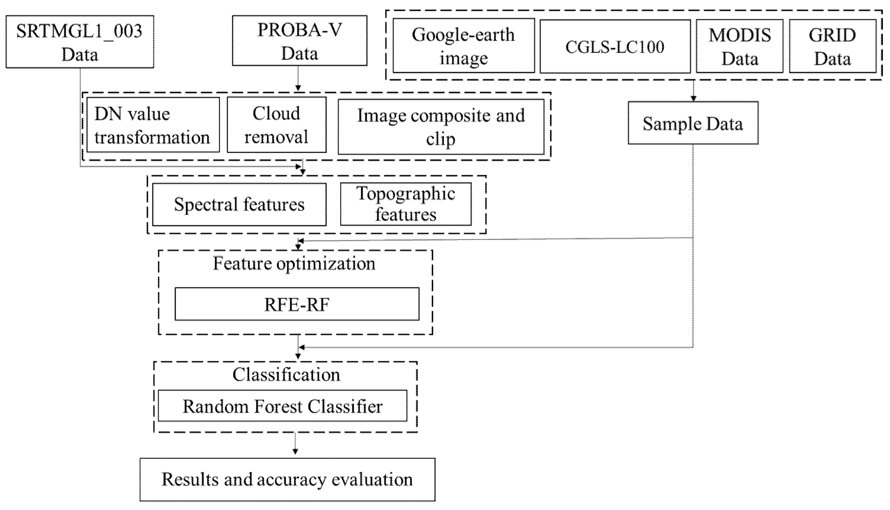
2. Materials and Methods
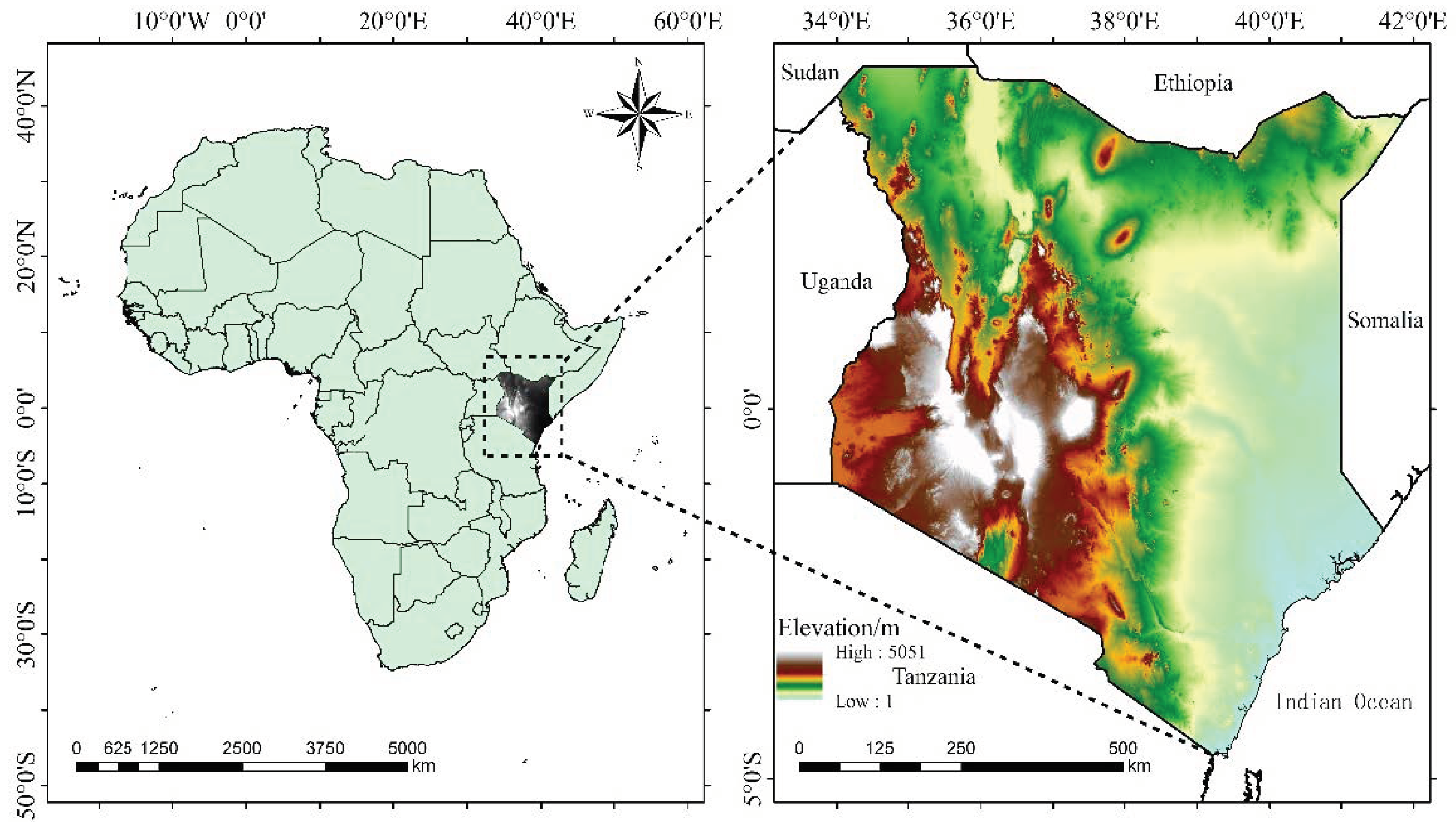
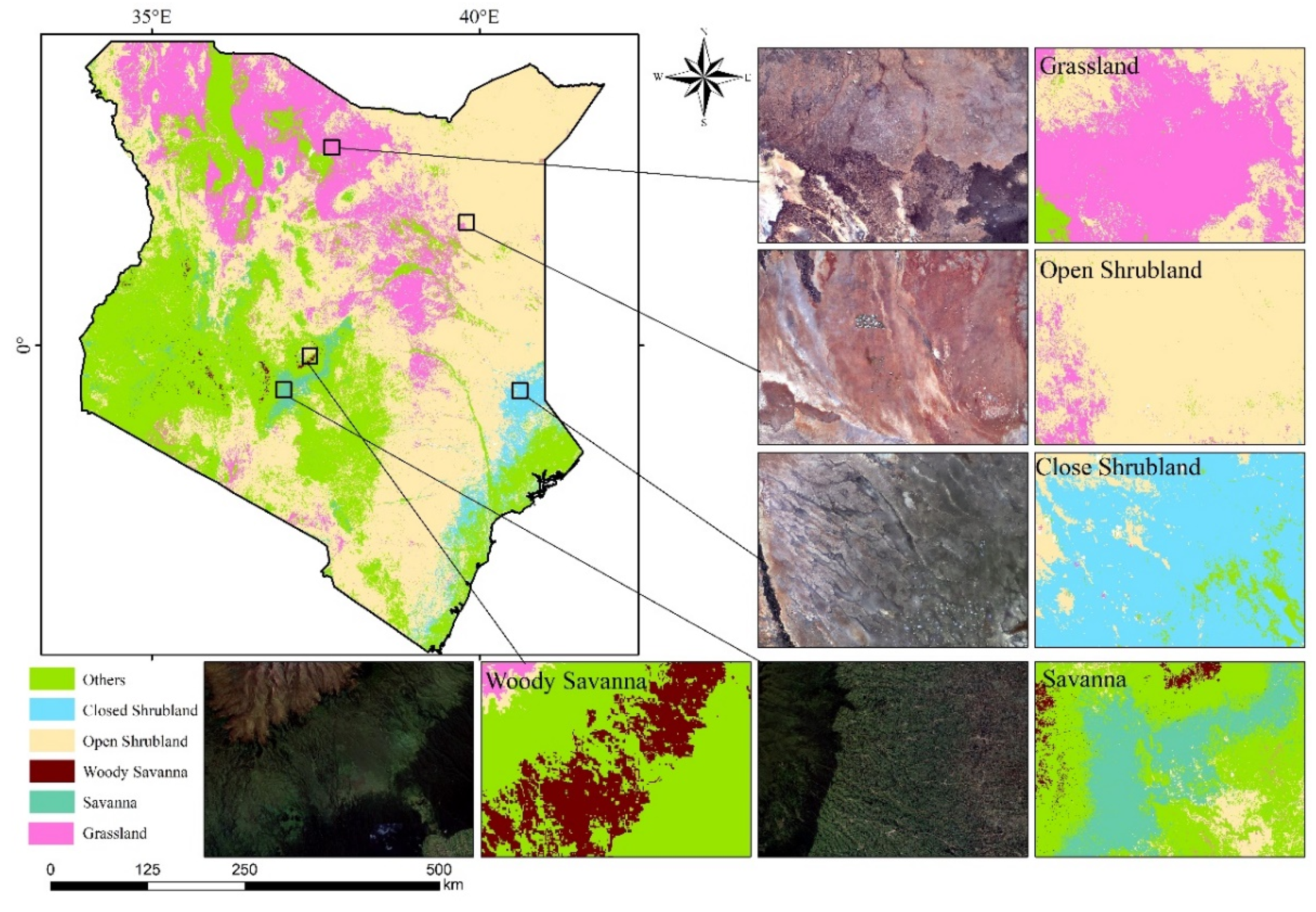
2.1. Study Area

Kenya is located in east of Africa (33°52′–41°53′E, 4°41′N–4°36′S, Area 582646m2), the equator crosses the center of Kenya, Somalia is to the east, Tanzania is to the south, Uganda is to the west, Ethiopia and South Sudan are to the north, and the Indian Ocean is to the southeast (as shown in Figure 1). Kenya was the African arrival point of China’s ancient Maritime Silk Road. The 800-km stretch of the East African Rift Valley runs north to south, with pearl-shaped lakes and volcanoes, plains with scrubs, grassland and farmland along the coast, and desert and semi-desert areas in the north. Kenya is located in a tropical monsoon zone, and most of the country has a savannah climate, with a humid climate in coastal areas and a mild climate in the highlands. Due to the monsoon climate, Kenya has no four distinct seasons, and only a difference between the rainy season and the dry season (the rainy season occurs from March to May and October to December, and the remaining months constitute the dry season). The annual rainfall decreases from 1500 mm to 200 mm from southwest to northeast, and the terrain greatly fluctuates. There are many rivers and lakes in Kenya, among which the Tana River is the longest river in Kenya.

2.2. Datasets and Processing

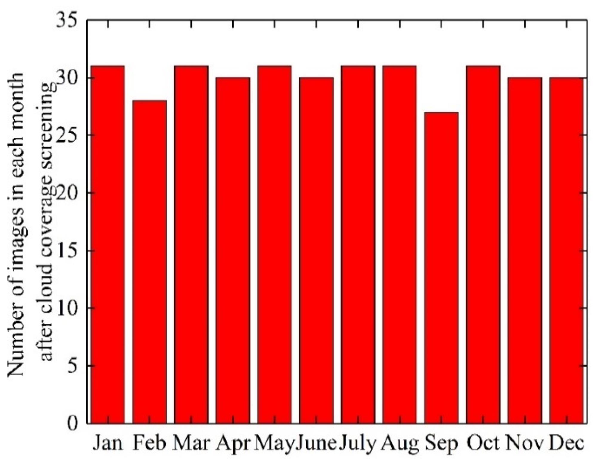
2.2.1. PROBA-V Image Data

On 7 May 2013, the ESA PROBA-V microsatellite, where V stands for vegetation, was successfully launched. The satellite has a size of 76 mm × 73 mm × 84 mm, a mass of 160 kg, and an inclination angle of 98.1° to its orbit. This satellite is the fourth in the PROBA series and is primarily used for global vegetation observation [25]. PROBA-V supports a number of applications, such as land cover, crop monitoring for global vegetation classification, forecasting, famine, food security, disaster management, and biosphere research [26]. Its spectral range is roughly the same as that of the SPOT series of vegetation sensors, but it has a higher spatial resolution. PROBA-V data are available in five bands: BLUE, RED, NIR, SWIR, and NDVI. The satellite provides daily images at 100 m and 333 m. A small amount of data and a larger number of available images are used in this paper. The data are based on the GEE platform for the relevant calculations. As the study area is located in the equatorial region, it receives more solar radiation and water vapor than other regions, and the vertical air currents develop more vigorously and has more cloud cover than other places. Therefore, the data are preprocessed, including converting the DN value of each band into reflectivity, cloud screening, etc. The cloud removal function is constructed according to the SM band in the data, and the data are processed. Because the study area distinguishes between rainy season and dry season, the images of rainy season and dry season are extracted respectively. The time span is 1 year, and the cloud amount is set to less than 20%. The figure below shows the number of images in each month after preprocessing (Figure 2).

2.2.2. SRTMGL1_003 Data

The Shuttle Radar Topography Mission (SRTM) [27] produces digital elevation data referred to as SRTUGL1_003, which are used to calculate elevation information for the study area. The data were provided by NASA JPL, with a spatial resolution of 30 m. It is converted to the same spatial resolution as the PROBA-V data by means of the resampling function in the GEE platform and finally cropped using Kenya’s boundary data.

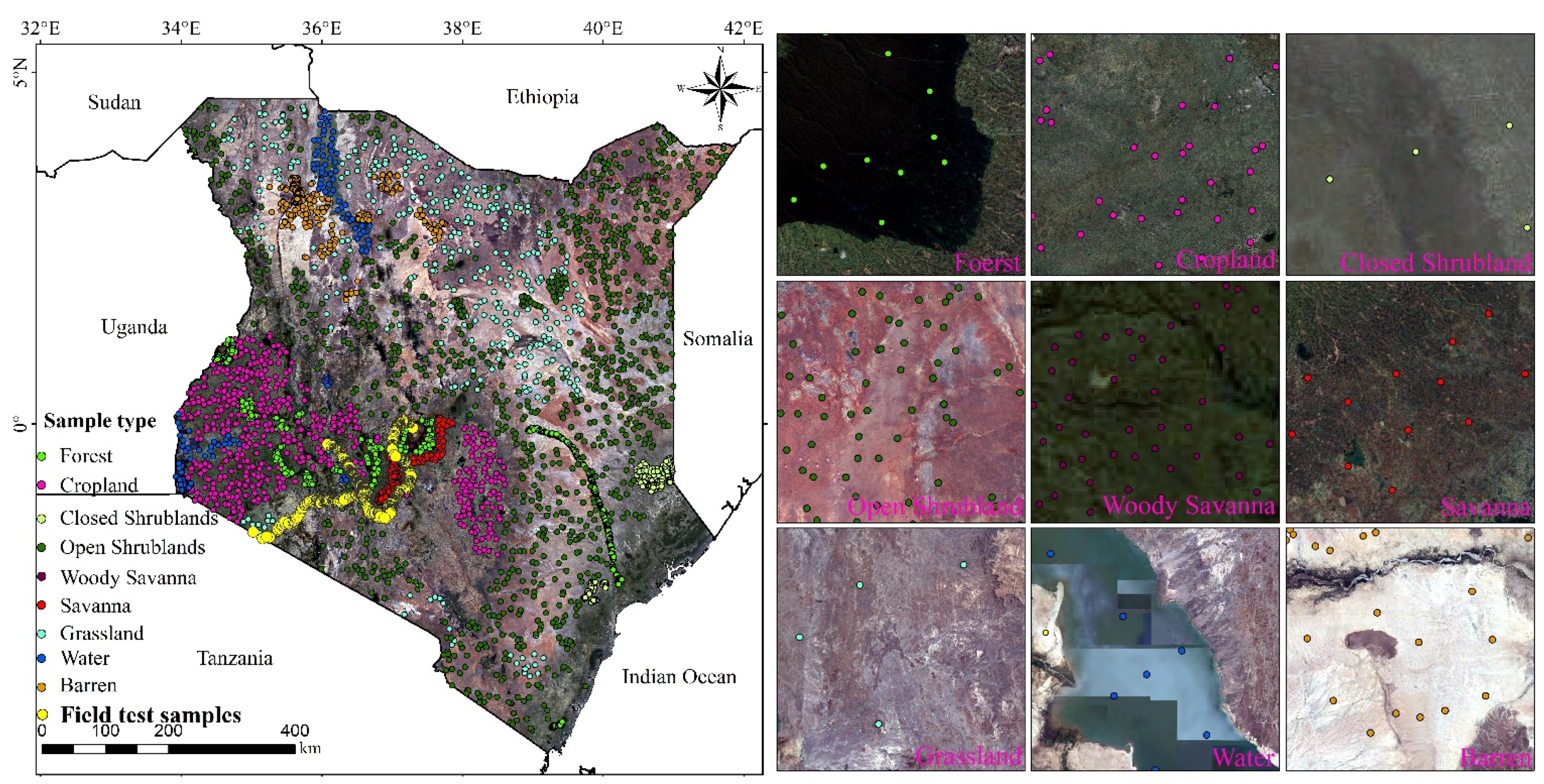
2.2.3. Sample Point Data
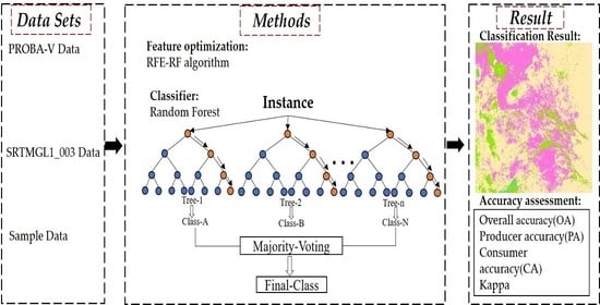
The classification system in this paper refers to the first land cover approach in the MCD12Q1 data (IGBP’s global vegetation classification scheme) and the project needs to divide land types into nine land classes: forest, cropland, water, barren, closed shrubland, open shrubland, woody savanna, savanna, and grassland.
The method of selecting samples only through visual interpretation cannot guarantee the objectivity of classification evaluation and the accuracy of samples. Therefore, sample data in this paper are determined by field survey data and existing data sets. Field survey data are obtained through GVG sampling (sampling time: 2018), and the existing data sets mainly include global land cover data (Forest Observations Europa, EU) provided by the European Commission and global dynamic land cover maps (CGLS-LC100) provided by the Copernicus Global Land Service, combined with high-resolution Google Earth images which were used to identify monitoring sites in Kenya, Africa. Nine types of sample points were selected (due to the small area of artificial surface coverage, the sample points were not listed separately), with a total of 3779 sample points (as shown in Table 1). There are 695 forest, 545 farmland, 263 closed shrubland, 1098 open shrubland, 237 woody savanna, 192 savanna, 360 grassland, 121 water and 268 bare. Then, the sample points were randomly divided into two parts: 50% of the sample points were used as training data sets, and the remaining 50% were used as validation data sets. Figure 3 shows the spatial distribution of various points and field sampling points.

2.3. Methods

In this paper, the remote sensing data of the study area were acquired and processed through the GEE platform, and the construction and optimization of spectral features and topographic features were completed. The random forest algorithm was used and the accuracy of the classification was evaluated to finally obtain the spatial distribution information of Kenya’s land cover in 2018. The technical flowchart of this paper is shown in Figure 4.

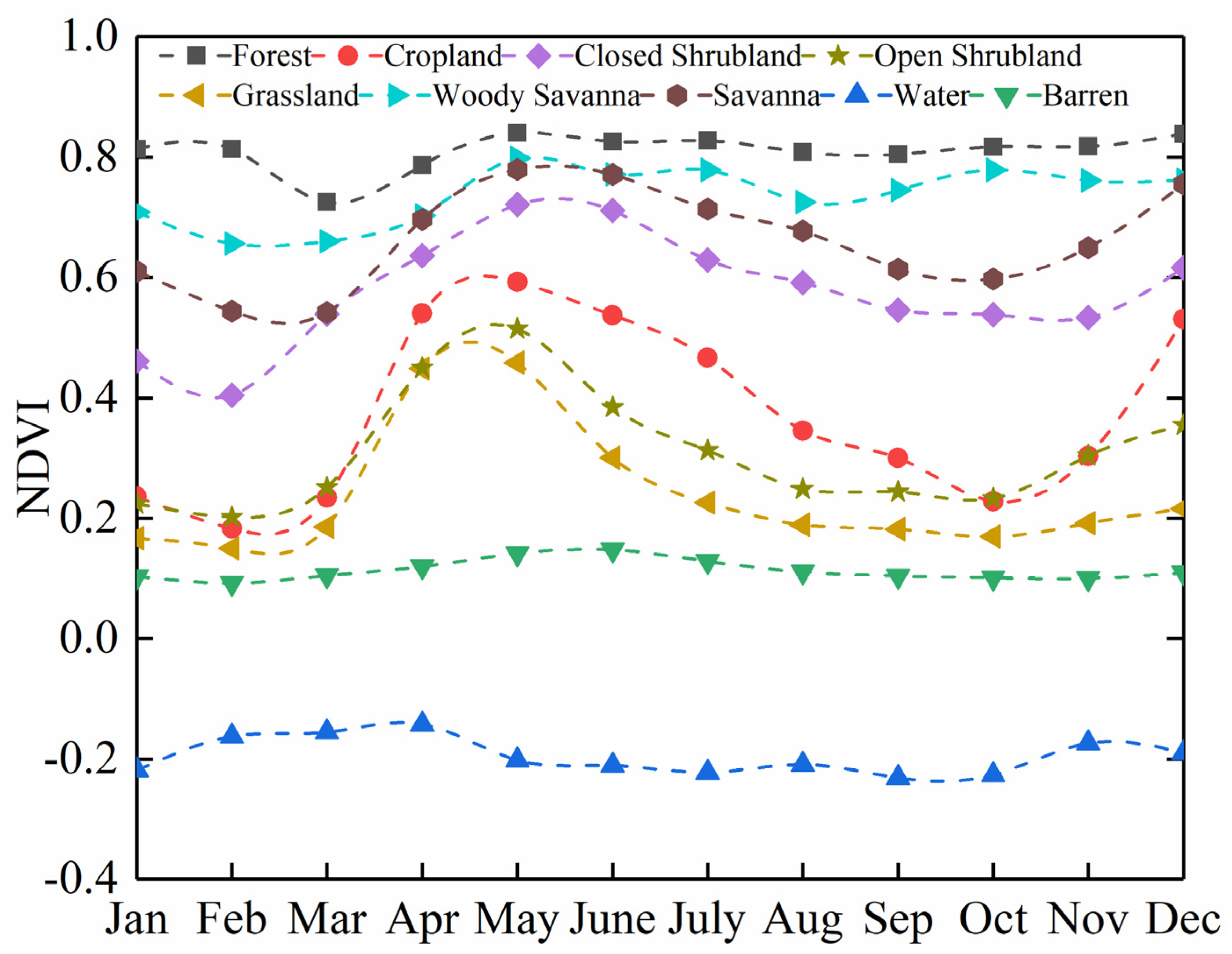
2.3.1. Spectral and Index Features

The selection of feature variables plays an important role in the classification process of remote sensing images. The appropriate use of multiple feature variables and combinations of feature variables can effectively improve the classification accuracy of remote sensing image [28]. In this paper, spectral features, index features, and topographic features are selected, and the following is the construction of these features on the GEE platform.
The spectral information of surface vegetation varies over time, so this paper analyses the effect of time on vegetation before constructing the spectral features. In this paper, monthly NDVI data were extracted for the dry and wet seasons and synthesized using the GEE platform for different land types. The graph below shows the variation of NDVI mean values for various land types in different months (as shown in Figure 5). As can be seen from the graph, the trend of NDVI curves for vegetation tends to be consistent, showing a rising–falling–rising trend, with an overall change in the alternation of wet–dry–wet seasons in the study area. The NDVI time series for water bodies and bare ground in the study area is relatively smooth and easily identifiable as it differs from other land types in the study area. March to May is the first rainy season of the year in the study area, also known as the ‘long rainy season’. The NDVI values of all vegetation species begin to rise. The short rainy season crops in Kenya are planted in December and harvested in February–March of the following year; therefore, the NDVI of farmland during this period is lower than that of grassland, followed by the planting of long rainy season crops, mainly wheat and maize, resulting in a higher NDVI in farmland than in grassland. In addition to this, the NDVI of open shrubland and grassland differed less between the two during this period, whereas during the dry season, the difference in NDVI values between the two was relatively large. Therefore, it is easier to achieve a classification for both in the dry season as opposed to the wet season. The NDVI values of woody savanna are consistently higher than those of savanna, but the difference between the two NDVI values during the wet season is also smaller, which is not conducive to better classification between the two. In summary, the dry season images were chosen for the identification of the study area as the NDVI values of some of the species in the study area differed less in the wet season and more in the dry season, making the dry season more favorable than the wet season for differentiating between the less diverse species.
After screening using the time, the location of the study area, and cloud removal, a total of 148 landscape images were obtained in the dry season, and each image contained 4 original spectral bands (Table 2) and a spectral index of NDVI. As the best indicator reflecting vegetation growth and coverage, NDVI is regarded as one of the effective indicators to monitor ecological environment and vegetation change. It not only eliminates the effects of satellite observation angles, solar elevation, topography, and cloud shadows, but it also reduces the effects of atmospheric and other related radiation changes. It has also been widely used for land use/cover classification, but the index is not sensitive when assessing areas with high vegetation cover and is prone to saturation problems. The EVI not only reduces the impact of soil background and aerosols, but also reduces the impact of saturated NDVI data. The LSWI can provide a reference indicator for the classification of water present in the study area. Kenya’s bare land is mainly distributed in the lack of rain of the northwest desert area. The ratio vegetation index (RVI) can accurately reflect the difference between the reflection of green vegetation in the visible band and near infrared band as well as the soil background. It can enhance the vegetation information, weaken the non-vegetation information and provide reference index for the classification of vegetation area and non-vegetation area. In summary, in this paper, NDVI, EVI, LSWI, and RVI were selected for the classification of different land cover patterns in Kenya, and the corresponding codes were written according to the formulae for calculating remote sensing indices. The band selection was prepared for subsequent classification. The various vegetation indices are calculated using the following formulae.
E V I = 2.5 × ρ N I R ρ R E D ρ N I R + 6 × ρ R E D 7.5 × ρ B L U E + 1
L S W I = ρ N I R ρ S W I R ρ N I R + ρ S W I R
RVI = ρ NIR ρ RED
where ρ N I R , ρ S W I R , ρ R E D , and ρ B L U E represent reflectance values in the NIR, SWIR, RED, and BLUE bands, respectively.

2.3.2. Topographic Features

Topography is an important basis for land resources. The undulation, slope, and aspect of land surface affect the distribution, planting structure, and soil erosion of forest land, farmland, and other land cover modes, and restrict the difficulty and mode of land resource utilization [29]. Therefore, the inclusion of topographic parameters as features in the later classification can improve the classification accuracy of land classes affected by topographic elements. This study uses SRTMGL1_003 data to construct four features: elevation, slope, slope orientation, and hill shading. These can be calculated using the ee. terrain. Products (input) function are provided by the GEE platform. This is then used as 4 separate bands to participate in the construction of the original features where the input to this function is the SRTMGL1_003 data.

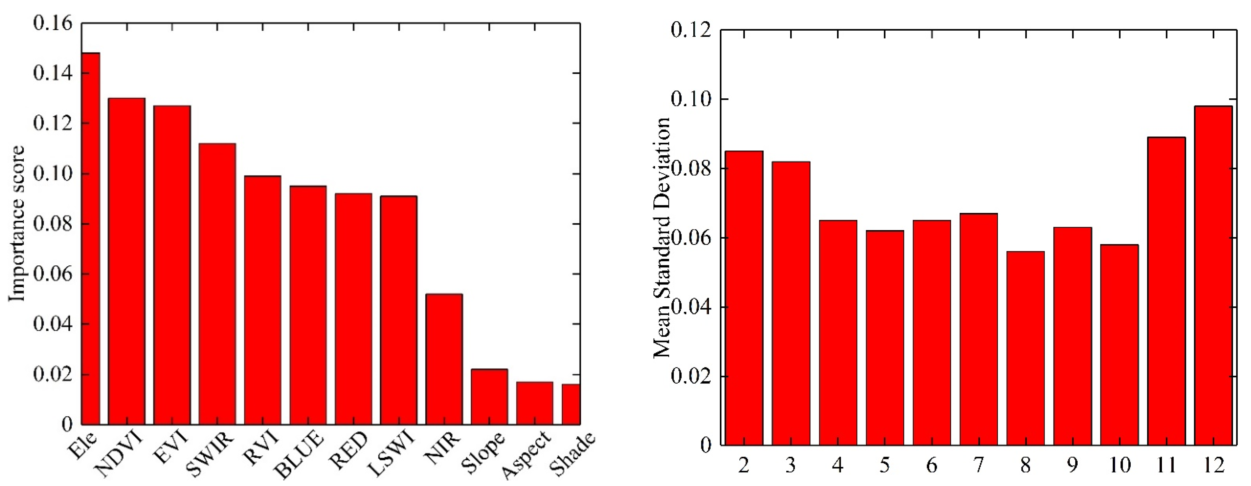
2.3.3. Feature Optimization Methods

There are tens, hundreds, or even more features used for remote sensing image classification. If all the features are involved in the training of the classifier, not only will the operation become cumbersome, which will greatly reduce the processing speed of the data, but also in the case of limited samples, too many features may lead to the reduction in the classification accuracy, which is called “dimensional disaster” [30,31]. It is therefore essential to optimize the features involved in image classification.
Recursive feature elimination (RFE) is a feature selection algorithm for packaging classification. The main purpose of RFE is to select the features that are most helpful for identifying and distinguishing the target object category in the study area. It can obtain as few input feature sets as possible without reducing the final classification accuracy. In this paper, forward iteration is used to optimize feature selection. It is a gradual process of feature addition, which requires all features to be ranked in order of importance first. Then, according to the characteristics of all order (according to the characteristics of the descending order of importance), the characteristics of the first importance to score high, modeling, and then gradually add the next characteristics, modeling, again from the current new feature set classification ability evaluation results. Until all features are added into the model, the feature set with the highest score and the least number of features is selected as the optimal feature set to participate in the final classification process. The stability of the algorithm largely depends on the model selected during iteration. Therefore, before feature optimization, this paper first compares the score and standard deviation of packaging algorithm formed by the RFE algorithm and several common algorithms, and then determines which common algorithm and packaging algorithm formed by RFE algorithm can achieve feature optimization.

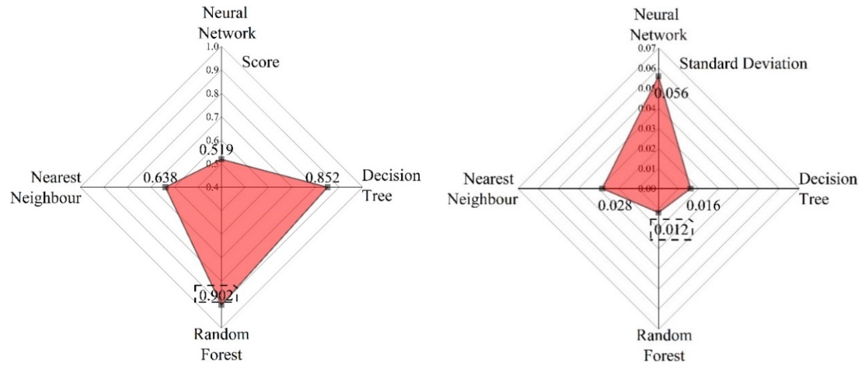
2.3.4. Classification Methods

Random Forest (RF) is an ensemble learning classifier, which is a machine learning algorithm formed by the combination of many CART decision trees and voting mechanisms [32]. Its greatest advantage lies in the importance of measurement variables [33]. The random forest algorithm uses a collection of classification trees to generate highly unbiased and accurate predictions based on voting across adaptive repetitions, which largely avoids overfitting [34]. When classifying remote sensing images, RF is faster to classify than other classifiers and easier to implement [35]. Its classification results are obtained by voting by multiple weak classifiers, so it is more robust than other classifiers. Random forest can also process continuous data and discrete data, and the data set does not need to be standardized. The introduction of two randomness makes the random forest not prone to overfitting of the decision tree, and at the same time it saves the pruning of the decision tree, and the computational burden is small. The advantages of random forest enable it to classify more complex remote sensing images, which is suitable for multi-category and multi-features [36,37,38]. In addition, it can also estimate the advantages of missing data [13]. Therefore, this article uses random forest classifiers to classify images.
A random forest is a classifier that uses multiple trees to train and predict samples. The classifier was proposed by Breiman and Cutler in 2011. It contains two important methods, namely random feature subspace and out-of-bag estimation [39]. The basic principles of the random forest algorithm are as follows. (1) with the bagging method, N samples from the original sample points are randomly selected and put back to form a new training sample point. When N is large enough, and about one third of the samples are not in the training sample point, these data are called out of bag (OOB) data. (2) Under the Gini coefficient minimum principle, multiple CART decision trees are constructed and random forest is formed by randomly selecting the subset of each node variable after N decision trees are split internally. (3) The generated random forest classifier is used to classify the data. For accuracy evaluation, when each sample belongs to the OOB sample, the number of votes is counted every time and the majority vote determines the classification category. Since the OOB sample does not participate in the establishment of a decision tree, it can be used to estimate prediction errors, to evaluate model performance, and to quantify the importance of variables using OOB errors [32,40].

2.3.5. Accuracy Verification Methods

The accuracy verification method used in this paper is the confusion matrix. The confusion matrix is a common method for verifying the accuracy of various land classifications and is also known as the error matrix, represented in the form of an N × N matrix. In this paper, after identifying nine land types, i.e., forest, cropland, water, barren, closed shrublands, open shrublands, woody savanna, savanna, and grassland, the accuracy of each type of grassland identified is evaluated using the confusion matrix, the overall accuracy (OA), producer accuracy/mapping accuracy (producer accuracy (PA)), consumer accuracy (UA), and kappa coefficient [41]. The calculation process is as follows:
O A = i = 1 n X i i n × 100 %
P A = X i i X i + × 100 %
U A = X i i X + i × 100 %
K a p p a = n i = 1 n   X i i i = 1 n X i + X + i n 2 i = 1 n X i + X + i
where X i i is the number of pixels in class i that are correctly classified, which in the confusion matrix is the number of images on the diagonal; X i + is the number of images classified in class i ; X + i is the number of true reference pixels in class i ; and N is the number of all pixels in the classification process.

3. Results

3.1. Feature Optimization Results

Commonly used classification algorithms include random forest algorithm, decision tree algorithms, neural network algorithms, and nearest neighbor algorithms [42]. The selection of different algorithms as iterative models affects the feature optimization in the later stage. Therefore, this paper first compares the scores and standard deviations of several different machine learning algorithms after RFE packing, and the results are shown in Figure 6. From the figure, it can be seen that the scores and standard deviations of different algorithms are different when they are wrapped by RFE. The recursive feature elimination-random forest algorithm (RFE-RF) and the recursive feature elimination decision tree algorithm have higher scores and smaller standard deviations. However, the former scored the highest in comparison. The score and standard deviation were 0.903 and 0.012, respectively. The standard deviation of the neural network-recursive feature elimination algorithm was the highest at 0.059. It is further illustrated that, compared with other algorithms combined with RFE, the stability of searching for the optimal feature combination is higher.
The process of using the RFE-RF algorithm for feature selection is as follows. The first is the process of random forest. The bootstrap sampling method is used to extract multiple samples from the original samples, and a decision tree is constructed for each bootstrap sample. All decision trees form a RF, and calculate feature importance in the model. Subsequently, the feature evaluation of forward iteration is introduced, corresponding features are added in sequence according to the feature importance score until all features are added to the model to participate in modeling, and finally the optimal feature combination participating in classification is determined. In the process of feature selection with the recursive feature elimination random forest algorithm (RFE-RF), the average standard deviation is used to evaluate the quality of the feature optimization results. In the process of feature selection by RFE-RF, the average standard deviation is used to evaluate the result of feature optimization. In the feature selection process, the first features selected were those with the top two feature importance scores, i.e., elevation and normalized difference vegetation index (NDVI), and the RFE-RF algorithm is used to calculate the mean standard deviation of feature optimization selection using these two features. Then, one feature was added in order of importance according to the remaining features, and the mean variance value of the added feature was calculated using RFE-RF algorithm until all 12 features participated in the modelling. After iteration, the optimal feature combination was selected according to the average standard deviation value. In Figure 7, it can be seen that, as the number of features continues to increase, the average standard deviation value shows the general trend of first decreasing and then increasing until the average standard deviation value reaches the maximum when all of the features are added. The larger the average standard deviation value, the less effective the RFE-RF is in optimizing the features. The optimal number of features after RFE-RF feature selection is eight, and the optimal feature combinations are elevation, NDVI, EVI, SWIR, RVI BLUE, RED, and LSWI. Table 3 shows the comparison of feature numbers before and after optimization by the RFE-RF algorithm.

3.2. Classification Results and Analysis

Based on the RFE-RF algorithm, nine land types in Kenya, Africa, including forest, farmland, water, barren, closed shrublands, open shrublands, woody savanna, savanna, and grassland, were extracted in 2018. As the research object of this paper is mainly grassland, forest, farmland, water, and barren, it is combined into other land types. The land cover classification map is shown in Figure 8. As can be seen from the map of land classification results, Kenya’s open shrublands are the most widespread of the five land cover types and are mainly found in the North Eastern province and parts of the Eastern and Rift Valley provinces of Kenya, with a few in the Western province within the study area. The next most widespread is grassland, which are mainly found in the Eastern and Rift Valley provinces of the study area. Closed shrublands, woody savanna, and savanna have a relatively small distribution range and are mainly distributed in parts of the Central province within the study area.
Table 4 shows the confusion matrix results for the classification. As can be seen from the table, out of the 1853 validation points selected, the true number of forest samples was 341, of which 314 were classified correctly and 27 were missed. The true sample number of cropland was 253, among which 223 were classified correctly and 30 were classified incorrectly. The spectrum of water differs greatly from that of other land types; thus, it is the best classification effect and there is no leakage phenomenon. There were 123 real samples of barren, of which 115 were classified correctly and 8 were missed. The true sample size for closed shrubland was 124, of which 112 were correctly classified and 12 were missed. The true sample size for open shrubland was 547, of which 478 were correctly classified and 69 were missed. The true sample size for woody savanna was 128, of which 115 were correctly classified and 13 were missed. The true sample size for savanna was 95, of which 84 were correctly classified and 11 were missed. The true sample size for grasslands was 182, of which 119 were correctly classified and 63 were missed. The producer accuracies of different land types can easily be deciphered as 0.92, 0.88, 0.90, 0.87, 0.89, 0.88, 0.65, 1, and 0.93, and it can be concluded that the errors of missing scores for the five land types were 0.08, 0.12, 0.10, 0.13, 0.11, 0.12, 0.35, 0, and 0.07. As can be seen above, water had the highest producer accuracy and the lowest omission error among the nine land classes. Of the five categories of grassland, closed shrubland had the highest classification accuracy, followed by savanna, woody savanna, and closed grassland, while grassland had the lowest classification accuracy and was mainly misclassified as open shrubland. The overall validation accuracy of the classification was 0.87, with a kappa coefficient of 0.85.

4. Discussion

4.1. Effect of Timing on Classification

Different vegetation types have different index characteristics in different time periods [43]. Therefore, the determination of the best time period is particularly important for image classification. This is because it can obtain better vegetation classification results according to the temporal characteristics of images [44]. The study area is divided into dry season and rainy season. It can be seen from Figure 5 that the index characteristics of arbor savanna and savanna, as well as open grass and grassland, are close in the rainy season, but there is a gap in the index characteristics in the dry season. Therefore, selecting the dry season image as the final classification image is conducive to improving the classification accuracy and obtaining better classification results. Table 5 and Table 6 are the confusion matrices obtained from the rainy season image and the whole season image, respectively. As can be seen from the table, the overall accuracy and Kappa coefficient of the grassland system classification in the study area by using images of rainy season are 0.83 and 0.79, respectively. Compared with the image classification results in the dry season, the overall accuracy decreased by 4% and kappa decreased by 6%. The overall accuracy of grassland system classification using whole-season images decreased by 1% and Kappa decreased by 2% compared with that using dry season images. Therefore, in image classification, it is necessary to select a reasonable time period for land type recognition based on the actual situation of the study area, which is conducive to improving the accuracy of land type recognition.

4.2. Effect of Auxiliary Data on Classification

Auxiliary data play a very important role in the process of improving the quality of mapping [45]. Cheng et al. [6] used a study on the remote sensing estimation method of a rice-planted area through the composite of the digital elevation model and multi-temporal MODIS data to find that the accuracy of the rice planted area estimated using single-view imagery was 53.3%, while the accuracy of rice planted area extracted using slope and MODIS-EVI index was 61.7%, an improvement of 8.4% over the former. He et al. [8] constructed topographic features and found that the introduced topographic features could improve the separability between land classes through the feature optimization algorithm, SEaTH algorithm, which in turn could improve the final classification accuracy. With the inclusion of elevation features in this study, the overall accuracy of the classification and the Kappa coefficient were both improved. Table 7 shows the confusion matrix obtained without the inclusion of elevation bands. As can be seen from the table, the overall accuracy is 0.84 and the Kappa coefficient is 0.81. This is a 3% decrease in overall accuracy and a 4% decrease in Kappa compared to the results obtained with the inclusion of elevation features in the image classification. Therefore, when classifying images, it is necessary to add auxiliary data reasonably in conjunction with the study area, which is conducive to improving the accuracy of the identification of land classes.

5. Conclusions

In combination with Google Earth Engine cloud platform, this paper obtained 2018 PROBA-V data covering Kenya in Africa over a short period of time and completed data pre-processing, including cloud removal, image Mosaic cutting, etc. In addition, spectral features and topographic features were constructed, and the features were optimized based on machine learning algorithm. Finally, five land types were classified in Kenya, Africa in 2018: closed shrubland, open shrubland, woody savanna, savanna, and grassland. The main conclusions are as follows.
(1) The GEE platform is a cloud-based planetary-scale geospatial analysis platform with advanced cloud computing and storage capabilities for dealing with various social hotspots, as well as easy and fast access to remote sensing data and other data resources, and the ability to process these data with the platform’s high-performance cloud computing capabilities. Based on this platform, this paper quickly implements pre-processing work such as ground time screening, cloud screening, de-clouding, compositing and cropping of dry season images in the study area, which has obvious advantages in terms of time compared to local processing.
(2) In this paper, machine learning algorithms are used in the feature combination optimization section, by comparing the scores and standard deviations of several commonly used algorithms with RFE combinations. In comparison, RFE has the highest score of 0.902 and the smallest standard deviation of 0.012 when combined with the random forest algorithm, thus providing the highest stability in modelling and the best optimization of features.
(3) After feature optimization by the RFE-RF algorithm, the number of features was reduced from the original 12 features to 8, which compressed the original feature space and reduced the redundancy of features. The optimal combination of features was elevation, RVI, EVI, SWIR, LSWI, NDVI, RED, and BLUE, and the overall accuracy and kappa coefficient were 0.87 and 0.85, respectively.
(4) As the main feature of the classification, the spectral features play a decisive role in the classification accuracy, and the appropriate use of auxiliary data can improve the classification accuracy. For the study area, the topographic features vary greatly among the local species, and the inclusion of topographic features is more conducive to the identification and classification of the local species.
In this study, PROBA-V data with spatial resolution of 100 m were used to explore the applicability of recursive feature elimination random forest algorithm, providing a new method for grassland monitoring with high spatial and temporal resolution. When using these data and RFE for classification, the following problems need to be highlighted. When using PROBA-V data for relevant research, it is necessary to convert pixel brightness value (DN) of remote sensing image into standard true value. When the RFE algorithm is used for feature optimization, the stability of the algorithm largely depends on the model selected during iteration. Selecting different models for iteration will have an impact on feature optimization. Therefore, iterate according to the actual model chosen. There is a “salt and pepper phenomenon” in the classification results based on pixels. In the later research focus, the RFE-RF algorithm and segmentation algorithm will be combined to achieve object-oriented classification of other regions.

Author Contributions

Conceptualization, P.W., W.Z., X.Z. and N.Y.; methodology, P.W., W.Z. and X.Z.; writing—original draft preparation, P.W., Y.Z., P.F. and H.Z.; writing—review and editing, X.Z. and N.Y.; supervision, W.Z., X.Z. and N.Y.; All authors have read and agreed to the published version of the manuscript.

Funding

This research was funded by the Strategic Priority Research Program of the Chinese Academy of Sciences (Grant No. XDA19030202), the National Key Research and Development Program of China (2021YFE0106700), the Key Technologies R&D Program of the Henan province (212102110033).

Institutional Review Board Statement

Not applicable.

Informed Consent Statement

Not applicable.

Data Availability Statement

PROBA-V data, SRTMGL1_003 data, CGLS-LC100 data and MODIS data are openly available via the Google Earth Engine, other data are available upon request from the first author.

Acknowledgments

We thank the data providers for this study: the PROBA-V data and the SRTMGL1_003 data were provided by ESA and NASA JPL.CGLS-LC100 data was provided Copernicus. MODIS data was provided by NASA LP DAAC at the USGS EROS Center and Google Earth Engine (GEE). We are grateful to the anonymous reviewers whose constructive suggestions have improved the quality of this study.

Conflicts of Interest

The authors declare that they have no known competing financial interests or personal relationships that could have appeared to influence the work reported in this paper.

References

  1. Chen, J.; Liu, Y.H.; Yu, Z.R. Planting Information Extraction of Winter Wheat Based on the Time-Series MODIS-EVI. J. Chin. Agric. Sci. Bull. 2011, 27, 446–450. [Google Scholar]
  2. Fang, P.; Zhang, X.; Wei, P.; Wang, Y.; Zhang, H.; Liu, F.; Zhao, J. The Classification Performance and Mechanism of Machine Learning Algorithms in Winter Wheat Mapping Using Sentinel-2 10 m Resolution Imagery. Appl. Sci. 2020, 10, 5075. [Google Scholar] [CrossRef]
  3. Fang, P.; Yan, N.; Wei, P.; Zhao, Y.; Zhang, X. Aboveground Biomass Mapping of Crops Supported by Improved CASA Model and Sentinel-2 Multispectral Imagery. Remote Sens. 2021, 13, 2755. [Google Scholar] [CrossRef]
  4. Liu, H. Extraction of crop planting structure in Hetao irrigated area based on Sentinel-2. J. Arid. Land Resour. Environ. 2021, 35, 88–95. [Google Scholar]
  5. Zhang, X.-W.; Liu, J.-F.; Qin, Z.; Qin, F. Winter wheat identification by integrating spectral and temporal information derived from multi-resolution remote sensing data. J. Integr. Agric. 2019, 18, 2628–2643. [Google Scholar] [CrossRef]
  6. Hao, P.; Wang, L.; Niu, Z. Comparison of Hybrid Classifiers for Crop Classification Using Normalized Difference Vegetation Index Time Series: A Case Study for Major Crops in North Xinjiang, China. PLOS ONE 2015, 10, e0137748. [Google Scholar] [CrossRef]
  7. Potgieter, A.B.; Apan, A.; Dunn, P.; Hammer, G. Estimating crop area using seasonal time series of Enhanced Vegetation Index from MODIS satellite imagery. Aust. J. Agric. Res. 2007, 58, 316–325. [Google Scholar] [CrossRef] [Green Version]
  8. Chen, Q.; Wang, R.C. Estimation of the rice planting area using digital elevation model and multitemporal moderate resolution imaging spectroradiometer. J. Trans. Chin. Soc. Agric. Eng. 2005, 5, 89–92. [Google Scholar]
  9. Zhang, X.; Qiu, F.; Qin, F. Identification and mapping of winter wheat by integrating temporal change information and Kullback–Leibler divergence. Int. J. Appl. Earth Obs. Geoinf. 2019, 76, 26–39. [Google Scholar] [CrossRef]
  10. He, Z.X.; Zhang, M.; Wu, B.F.; Xing, Q. Extraction of Summer Crop in Jiangsu based on Google Earth Engine. J. Geo-Inf. Sci. 2019, 21, 752–766. [Google Scholar]
  11. Huang, D.S. Research on Feature Selection and Semi-Supervised Classification. Ph.D. Thesis, Huazhong University of Science and Technology, Wuhan, China, 2011. [Google Scholar]
  12. Liu, H.; Yu, L. Toward integrating feature selection algorithms for classification and clustering. IEEE Trans. Knowl. Data Eng. 2005, 17, 491–502. [Google Scholar]
  13. Liu, X.X. Study on the Remote Sensing Feature Selection Method for Forest Biomass Estimation Based on RF-RFE. Master’s Thesis, Shandong Agricultural University, Tai’an, China, 2016. [Google Scholar]
  14. Guyon, I.; Weston, J.; Barnhill, S. Gene Selection for Cancer Classification using Support Vector Machines. J. Mach. Learn. 2002, 46, 389–422. [Google Scholar] [CrossRef]
  15. Lou, P.; Fu, B.; He, H.; Li, Y.; Tang, T.; Lin, X.; Fan, D.; Gao, E. An Optimized Object-Based Random Forest Algorithm for Marsh Vegetation Mapping Using High-Spatial-Resolution GF-1 and ZY-3 Data. Remote Sens. 2020, 12, 1270. [Google Scholar] [CrossRef] [Green Version]
  16. Demarchi, L.; Kania, A.; Ciężkowski, W.; Piórkowski, H.; Oświecimska-Piasko, Z.; Chormański, J. Recursive Feature Elimination and Random Forest Classification of Natura 2000 Grasslands in Lowland River Valleys of Poland Based on Airborne Hyperspectral and LiDAR Data Fusion. Remote Sens. 2020, 12, 1842. [Google Scholar] [CrossRef]
  17. Han, L.; Yang, G.; Dai, H.; Xu, B.; Yang, H.; Feng, H.; Li, Z.; Yang, X. Modeling maize above-ground biomass based on machine learning approaches using UAV remote-sensing data. Plant Methods 2019, 15, 1–19. [Google Scholar] [CrossRef] [Green Version]
  18. Luo, M.; Wang, Y.; Xie, Y.; Zhou, L.; Qiao, J.; Qiu, S.; Sun, Y. Combination of Feature Selection and CatBoost for Prediction: The First Application to the Estimation of Aboveground Biomass. Forests 2021, 12, 216. [Google Scholar] [CrossRef]
  19. Pullanagari, R.R.; Kereszturi, G.; Yule, I. Integrating Airborne Hyperspectral, Topographic, and Soil Data for Estimating Pasture Quality Using Recursive Feature Elimination with Random Forest Regression. Remote Sens. 2018, 10, 1117. [Google Scholar] [CrossRef] [Green Version]
  20. An, Y.; Chen, G.F.; Li, J. Research on Soybean Pre-Micro RNA Prediction Model Based on Recursive Feature Elimination and Random Forest Fusion Algorithm. J. Soybean Sci. 2020, 39, 401–405. [Google Scholar]
  21. Dai, H.; Fu, R.D.; Jin, W. Glioma grading prediction based on radiomics and ensemble learning. J. Ningbo Univ. (Nat. Sci. Eng. Ed.) 2021, 34, 28–34. [Google Scholar]
  22. Huang, X.; Zhang, L.; Wang, B.; Li, F.; Zhang, Z. Feature clustering-based support vector machine recursive feature elimination for gene selection. Appl. Intell. 2018, 48, 594–607. [Google Scholar] [CrossRef]
  23. Johannes, M.; Brase, J.C.; Fröhlich, H.; Gade, S.; Gehrmann, M.; Fälth, M.; Sültmann, H.; Beißbarth, T. Integration of pathway knowledge into a reweighted recursive feature elimination approach for risk stratification of cancer patients. Bioinformatics 2010, 26, 2136–2144. [Google Scholar] [CrossRef] [Green Version]
  24. Schlosser, A.; Szabó, G.; Bertalan, L.; Varga, Z.; Enyedi, P.; Szabó, S. Building Extraction Using Orthophotos and Dense Point Cloud Derived from Visual Band Aerial Imagery Based on Machine Learning and Segmentation. Remote Sens. 2020, 12, 2397. [Google Scholar] [CrossRef]
  25. Song, R. Successful launch of ESA proba-v microsatellite. J. Spacecr. Recovery Remote Sens. 2013, 34, 81. [Google Scholar]
  26. Cao, X.J. Study on Phenology Monitoring and Pest Response of Pinus Yunnanensis Based on Multi-source Remote Sensing Data Fusion. Master’s Thesis, Beijing Forestry University, Beijing, China, 2018. [Google Scholar]
  27. Farr, T.G.; Rosen, P.A.; Caro, E.; Crippen, R.; Duren, R.; Hensley, S.; Seal, D. The shuttle radar topography mission. Rev. Geophys. 2007, 45, 361. [Google Scholar] [CrossRef] [Green Version]
  28. Jia, K.; Li, Q.Z. Review of Features Selection in Crop Classification Using Remote Sensing Data. J. Resour. Sci. 2013, 35, 2507–2516. [Google Scholar]
  29. Song, K.S.; Liu, D.W.; Zhang, B.; Wang, Z.M.; Li, F.; Zhang, S.Q.; Zhang, C.-h.; Yang, T. Impacts of Topographic Features on Landuse/Cover Change in Sanjiang Plain. Bull. Soil Water Conserv. 2008, 28, 2, 10–15. [Google Scholar]
  30. Zhang, X.Y.; Feng, X.Z.; Jiang, H. Feature set optimization in object-oriented methodology. J. Remote Sens. 2009, 13, 659–669. [Google Scholar]
  31. De Sa, J.M. Pattern Recognition: Concepts, Methods and Applications; Springer Science & Business Media: Berlin, Germany, 2012. [Google Scholar]
  32. Bierman, L. Random Forests. Mach. Learn 2001, 45, 5–32. [Google Scholar] [CrossRef] [Green Version]
  33. Xiangyu, G.; Jianli, D.; Jingzhe, W.; Fei, W.; Lianghong, C.; Huilan, S. Estimation of Soil Moisture Content Based on Competitive Adaptive Reweighted Sampling Algorithm Coupled with Machine Learning. Acta Opt. Sin. 2018, 38, 393–400. [Google Scholar] [CrossRef]
  34. Yan-bing, Q.; Yin-yin, W.; Yang, C.; Jiao-Jiao, L.; Liang-Liang, Z. Soli Orfanic Matter Prediction Based on Remote Sensing Data and Random Forest Model in Shaanxi Province. J. Nat. Resour. 2017, 32, 1074–1086. [Google Scholar]
  35. Roy, D.; Kovalskyy, V.; Zhang, H.; Vermote, E.; Yan, L.; Kumar, S.S.; Egorov, A. Characterization of Landsat-7 to Landsat-8 reflective wavelength and normalized difference vegetation index continuity. Remote Sens. Environ. 2016, 185, 57–70. [Google Scholar] [CrossRef] [Green Version]
  36. Feng, Q.; Liu, J.; Gong, J. UAV Remote Sensing for Urban Vegetation Mapping Using Random Forest and Texture Analysis. Remote Sens. 2015, 7, 1074–1094. [Google Scholar] [CrossRef] [Green Version]
  37. Yue, M.; Qigang, J.; Zhiguo, M.; Yuanhua, L.; Dong, W.; Huaxin, L. Classification of Land Use in Farming Area Based on Random Forest Algorithm. Trans. Chin. Soc. Agric. Mach. 2016, 47, 297–303. [Google Scholar]
  38. Rodriguez-Galiano, V.F.; Olmo, M.C.; Abarca-Hernandez, F.; Atkinson, P.; Jeganathan, C. Random Forest classification of Mediterranean land cover using multi-seasonal imagery and multi-seasonal texture. Remote Sens. Environ. 2012, 121, 93–107. [Google Scholar] [CrossRef]
  39. Chan, J.C.-W.; Paelinckx, D. Evaluation of Random Forest and Adaboost tree-based ensemble classification and spectral band selection for ecotope mapping using airborne hyperspectral imagery. Remote Sens. Environ. 2008, 112, 2999–3011. [Google Scholar] [CrossRef]
  40. van Beijma, S.; Comber, A.; Lamb, A. Random forest classification of salt marsh vegetation habitats using quad-polarimetric airborne SAR, elevation and optical RS data. Remote Sens. Environ. 2014, 149, 118–129. [Google Scholar] [CrossRef]
  41. Giles, M. Foody, Status of land cover classification accuracy assessment. Remote Sens. Environ. 2002, 80, 185–201. [Google Scholar] [CrossRef]
  42. Zheng, X. Three Common Classification Algorithms and Their Comparative Analysis. J. Chongqing Univ. Sci. Technol. (Nat. Sci. Ed.) 2020, 22, 101–106. [Google Scholar]
  43. Song, Q.; Hu, Q.; Zhou, Q.; Hovis, C.; Xiang, M.; Tang, H.; Wu, W. In-Season Crop Mapping with GF-1/WFV Data by Combining Object-Based Image Analysis and Random Forest. Remote Sens. 2017, 9, 1184. [Google Scholar] [CrossRef] [Green Version]
  44. Senf, C.; Leitão, P.J.; Pflugmacher, D.; van der Linden, S.; Hostert, P. Mapping landcover in complex Mediterranean landscapes using Landsat: Improved classification accuracies from integrating multi-seasonal and synthetic imagery. Remote Sens. Environ. 2015, 156, 527–536. [Google Scholar] [CrossRef]
  45. Zhao, Y.Y.; Feng, D.L.; Yu, L.; Wang, X.Y.; Chen, Y.L.; Bai, Y.Q.; Hernandez, H.J.; Galleguillos, M.; Estades, C.; Biging, G.S.; et al. Detailed dynamic land cover mapping of Chile: Accuracy improvement by integrating multi-temporal data. Remote Sens. Environ. 2016, 183, 170–185. [Google Scholar] [CrossRef]
Figure 1. Geographical location of the study area.
Remotesensing 13 04762 g001
Figure 2. Number of images in each month after preprocessing.
Remotesensing 13 04762 g002
Figure 3. Sample point spatial distribution map.
Remotesensing 13 04762 g003
Figure 4. Technical flowchart.
Remotesensing 13 04762 g004
Figure 5. NDVI change graph of the mean value of different land types.
Remotesensing 13 04762 g005
Figure 6. RFE packaging algorithm score and standard deviation.
Remotesensing 13 04762 g006
Figure 7. Feature significance and mean standard deviation change diagram.
Remotesensing 13 04762 g007
Figure 8. Classification result diagram.
Remotesensing 13 04762 g008
Table 1. Sample point data.
Ground Class CodeLand Class NameNumber of Samples
1Water121
2Savanna192
3Woody savanna237
4Closed shrubland263
5Barren268
6Grassland360
7Cropland545
8Forest695
9Open shrubland1098
Table 2. Band parameters of PROBA-V data.
PROBA-V Spectral Bands Centred at (nm)Width Span (nm)
BLUE46346
RED65579
NIR85144
SWIR160073
Table 3. Original features and optimized features.
Features TypeOriginal FeaturesNumberOptimized FeaturesNumber
Spectral featuresBLUE, RED, NIR, SWIR4BLUE, RED, SWIR3
Index featuresNDVI, EVI, LSWI, RVI4NDVI, EVI, LSWI, RVI4
Topographic featuresElevation, Aspect, Slope, Hillshade4Elevation1
Total 12 8
Table 4. Confusion matrix.
Confusion
Matrix
Forecast Category
123456789TotalPA
Category13145351130003410.92
28223017050002530.88
3801124000001240.90
413154780030025470.87
51300011500001280.89
64700084000950.88
70405400119051820.65
80000000600601
9000300501151230.93
Total34827012056112692154601221853
UA0.900.820.930.850.910.910.7710.94
OA0.87
Kappa 0.85
Note: 1. forest; 2. cropland; 3. closed shrubland; 4. open shrubland; 5. woody savanna; 6. savanna; 7. grassland; 8. water; 9. barren.
Table 5. Confusion matrix.
Confusion
Matrix
Forecast Category
123456789TotalPA
Category130121071000003300.91
272470381100003030.81
3801189000001350.87
442584780333005510.86
517000810000980.82
65902074000900.82
7240870099041960.50
80000000600601
9000400501281370.93
Total3442871366259287137601321900
UA0.870.860.860.760.880.850.7210.96
OA0.83
Kappa 0.79
Note: 1. forest; 2. cropland; 3. closed shrubland; 4. open shrubland; 5. woody savanna; 6. savanna; 7. grassland; 8. water; 9. barren.
Table 6. Confusion matrix.
Confusion
Matrix
Forecast Category
123456789TotalPA
Category1325540900003430.94
27237021064002750.86
31301033000001190.86
4516135190030005830.89
5150009800001130.86
61217000790001080.73
70358000113031770.63
80000000570571
9000600801381520.90
Total37727817854910785155571411927
UA0.860.850.570.940.910.920.7210.97
OA0.86
Kappa0.83
Note: 1. forest; 2. cropland; 3. closed shrubland; 4. open shrubland; 5. woody savanna; 6. savanna; 7. grassland; 8. water; 9. barren.
Table 7. Confusion matrix.
Confusion
Matrix
Forecast Category
123456789TotalPA
Category130724311540003540.86
219222124090002750.80
3101295000001350.95
4625104390034055190.84
51100010600001170.90
601100083000940.88
72416400104091840.56
80000000580581
9000200401221280.95
Total34628614454511196142581361864
UA0.880.770.890.800.950.860.7310.89
OA0.84
Kappa 0.81
Note: 1. forest; 2. cropland; 3. closed shrubland; 4. open shrubland; 5. woody savanna; 6. savanna; 7. grassland; 8. water; 9. barren.
Publisher’s Note: MDPI stays neutral with regard to jurisdictional claims in published maps and institutional affiliations.

