Article

Temporal Information Extraction for Afforestation in the Middle Section of the Yarlung Zangbo River Using Time-Series Landsat Images Based on Google Earth Engine

1
Institute of Mountain Hazards and Environment, Chinese Academy of Sciences, Chengdu 610041, China
2
College of Earth Sciences, Chengdu University of Technology, Chengdu 610059, China
3
Kathmandu Center for Research and Education, Chinese Academy of Sciences-Tribhuvan University, Beijing 100101, China
4
University of Chinese Academy of Sciences, Beijing 100049, China
*
Author to whom correspondence should be addressed.
Remote Sens. 2021, 13(23), 4785; https://doi.org/10.3390/rs13234785
Submission received: 12 November 2021 / Revised: 22 November 2021 / Accepted: 24 November 2021 / Published: 25 November 2021
(This article belongs to the Special Issue Remote Sensing of Ecosystems)

Abstract

:
Afforestation is one of the most efficient ways to control land desertification in the middle section of the Yarlung Zangbo River (YZR) valley. However, the lack of a quantitative way to record the planting time of artificial forest (AF) constrains further management for these forests. The long-term archived Landsat images (including the Thematic Mapper (TM), Enhanced Thematic Mapper Plus (ETM+), and Operational Land Imager (OLI)) provide a good opportunity to capture the temporal change information about AF plantations. Under the condition that there would be an abrupt increasing trend in the normalized difference vegetation index (NDVI) time-series curve after afforestation, and this characteristic can be thought of as the indicator of the AF planting time. To extract the indicator, an algorithm based on the Google Earth Engine (GEE) for detecting this trend change point (TCP) on the maximum NDVI time series within the growing season (May to September) was proposed. In this algorithm, the time-series NDVI was initially smoothed and segmented into two subspaces. Then, a trend change indicator Sdiff was calculated with the difference between the fitting slopes of the subspaces before and after each target point. A self-adaptive method was applied to the NDVI series to find the right year with the maximum TCP, which is recorded as the AF planting time. Based on the proposed method, the AF planting time of the middle section of the YZR valley from 1988 to 2020 was derived. The detected afforestation temporal information was validated by 222 samples collected from the field survey, with a Pearson correlation coefficient of 0.93 and a root mean squared error (RMSE) of 2.95 years. Meanwhile, the area distribution of the AF planted each year has good temporal consistency with the implementation of the eco-reconstruction project. Overall, the study provides a good way to map AF planting times that is not only helpful for sustainable management of AF areas but also provides a basis for further research on the impact of afforestation on desertification control.

1. Introduction

As the social and economic center of Tibet [1], the middle section of the Yarlung Zangbo River (YZR) valley faces serious desertification due to intensive human activities and the fragile natural environment [2,3]. According to the statistics in Liu, et al. [4], there is a total of 2324.43 km2 of aeolian sand in the middle part of the YZR basin, especially on the north bank of the wide valleys. To control desertification, the local government has launched many ecological protection and construction projects since the 1980s, including planting artificial forest (AF), artificial shrub, and artificial grassland for sand stabilization [5].
Ecological construction provides a natural laboratory to explore the impact of afforestation on natural environment improvement. To some extent, AF is of great importance in carbon sequestration [6,7,8], desertification control [9], soil improvement [10,11,12], climate regulation [13,14], and biodiversity conservation [15,16]. To investigate the detailed impact of afforestation on the local eco-environment, it is necessary to compare the environmental indicators change before and after the AF plantation [17,18]. Therefore, the AF planting time is the basic information for related researches between AF and the local environment, especially under the background of significant climate change on the Tibetan Plateau [19,20].
However, the AF plantation regions are sparsely distributed and the planting activities, including renewal and maintenance, have continued for a long period. Most of the afforestation information has been recorded manually without full spatial or temporal details. Consequently, it is difficult to obtain the exact planting time for each AF patch. Although tree-ring measurement can reveal temporal information, this point-based measurement cannot provide comprehensive AF spatial-temporal distribution recordation. Currently, the lack of this temporal information greatly constrains the assessment of the effect of ecological projects and the improvement for future ecological conservation activity. The afforestation in the YZR is conducted via transplanting the cultivated seedlings to the sandy area to improve soil conditions and avoid desertification with the increase of vegetation coverage at the same time. Therefore, the AF planting time can be reflected by the time when the land cover type transfers from sand to AF.
In recent decades, the openly available long-term remote sensing image archives, such as the Landsat satellite image archive [21,22] and the MODIS satellite image archive [23,24,25], recorded long terms of land cover changes which make the AF planting time detection possible. In the time-series remote sensing images, the land cover change caused by afforestation mentioned above is represented by the trend change of the temporal vegetation index. Taking the time-series normalized difference vegetation index (NDVI) as an example, the time-series NDVI retained a flat trend during the sandy period, while an increasing trend after AF plantation. Therefore, the trend change point (TCP) in time-series NDVI can be used to represent the AFs planting time.
In addition, the rapid development of remote sensing technology has provided efficient methods for forest monitoring, including forest mapping [26], forest change [27], and forest health assessment [28]. Kennedy, et al. [29] developed an algorithm called LandTrendr and proposed the concept of tracking time-series images to detect forest changes. Fensholt, et al. [30] applied NDVI data from different platforms (NOAA, Terra, and SPOT) to conduct temporal-sequence analysis for long-term vegetation study. Huang, et al. [31] developed an algorithm called Vegetation Change Tracker (VCT) to monitor forest changes automatically using the Landsat time series stack (LTSS). Ochtyra, et al. [32] developed an algorithm called TVCMA and adopted a mixed-method based on deviation (threshold) and trend (regression) to detect vegetation changes. These detection methods perform well in temporal data change detection.
However, many factors, such as atmospheric noise and radiometric correction residuals distort the actual surface reflectance, causing outlier existence in the time-series NDVI [33]. These outliers usually existed with smaller duration and greater change degrees, which is easy to confuse with the AF plantation change pattern. Therefore, a trend change detection method is needed to express the change condition around each probe point while eliminating the influence of outliers.
In this study, aiming to map the AF planting times in the middle section of the YZR valley, an algorithm was proposed under the support of the Google Earth Engine (GEE) platform that tracks the temporal trend of the vegetation index acquired from long-term Landsat images. The basis of this research is that an abrupt increasing trend appears in the vegetation index curve after afforestation compared with the original sandy surface, and the AF planting time is detected by determining the time of this increase. Meanwhile, the outliers were reduced by an adaptive window smooth and subspace segmentation performed on the NDVI time series. With the developed method, a map of the AF spatial distribution and the AF planting time of the middle section of the YZR valley is acquired.

2. Study Area and Datasets
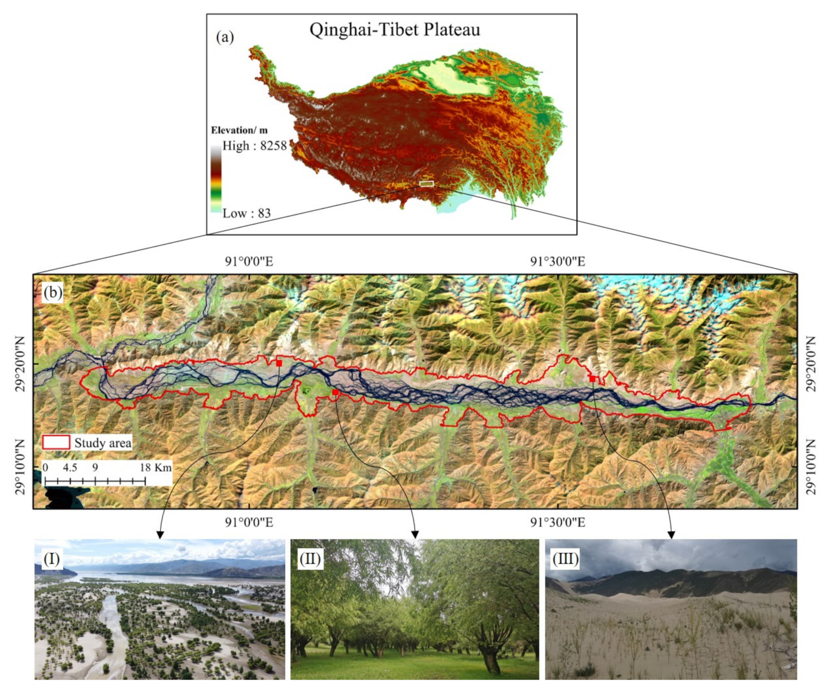
2.1. Study Area

The middle section of the YZR valley is located in the south of the Qinghai-Tibet Plateau (Figure 1a). This region is characterized by widely distributed sandy land, and land desertification is still an important environmental problem under the impact of human activities and climate change [34]. Therefore, the floodplain and sandy bank in this region have been planted with plenty of AFs to control desertification. As shown in Figure 1b, the study area surrounded by the red polygon has many green patches according to the Landsat-8 true-color image in 2020. Pictures of typical AF sites representing the AFs planted at different times are shown in Figure 1. Picture (I) shows the widely distributed AF planted on the riverbed. Picture (II) shows the mature AF with high vegetation cover. Picture (III) shows a newly planted AF.

2.2. NDVI Image Stack

To effectively capture the AF planting information, Landsat images acquired from the Landsat surface reflectance (Landsat-SR) product provided in the GEE platform were used in this study. In GEE, the Landsat-SR images operation was controlled by the internet-accessible application programming interactive (API) or the web-based interactive development environment (IDE), and the images were stored in the Google server and processed by the powerful parallel computing capability [35]. However, there are frequent clouds in the growing season (1 May to 30 September) because of the monsoon climate. Therefore, the cloud-free pixels were identified by the quality assessment (QA) band of the Landsat SR and used to form a composite cloud-free maximum NDVI image each year, for the maximum composite can be used to remove the effects of cloud-cover, scan-angle, and solar-zenith-angle [36], and reflect the true growth condition of the vegetation [37]. The QA band was derived from the C code based on the Function of Mask (CFMASK) [38] algorithm implemented on the Landsat images to mask the score of the cloud, cloud shadow, and snow et al.
The earliest observation of the study area dated back to 1988. For this long-term NDVI series, they were derived from different Landsat platforms. To balance the systematic biases among different Landsat sensors, the inter-calibration coefficients proposed by Roy, et al. [39] were applied to each band of OLI images to reduce the effect caused by the difference between the sensors TM, ETM+, and OLI.

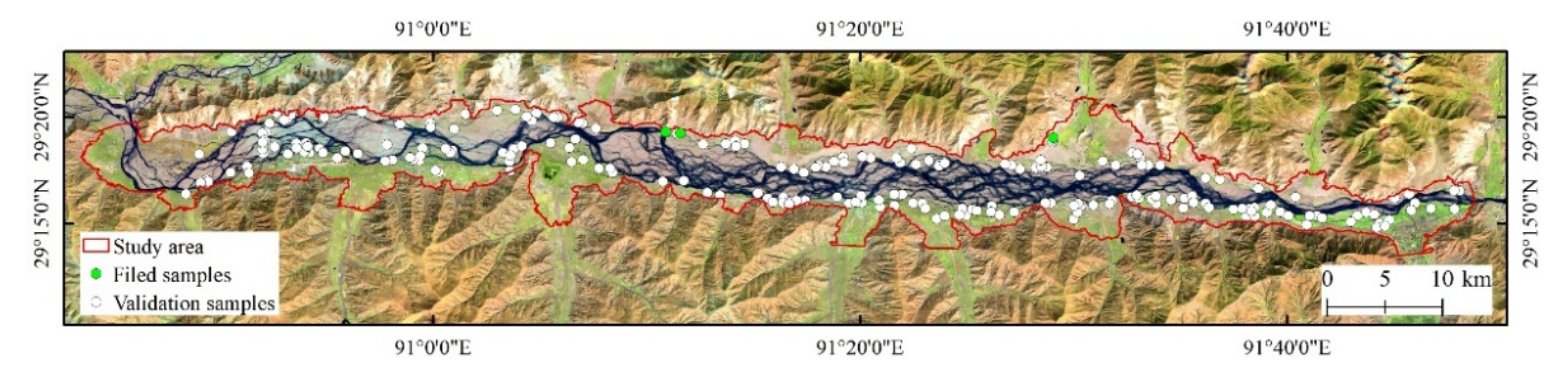
2.3. Validation Samples

To validate the mapping results of the planting time, a field survey was conducted from 8 to 15 August 2020, and the key AF patches (222 samples) were recorded by a handheld GPS (Figure 2). Then, the planting time of these samples was artificially determined from the time-series annual maximum NDVI in the growing season extracted from the GEE platform. Among these samples, three AF patches are clearly indicated by a signboard around them which mentioned the exact planting year and they are noted with green color in Figure 2.

3. Methods

The mapping of the AF planting time was conducted via the following two steps: (1) AF extraction and (2) planting time detection. In the first step, several spectral indices related to the key land cover types in this region were calculated firstly with the cloud-free image in 2020 and imported into a random forest classifier to extract AF regions. The indices include NDVI, normalized difference sand index (NDSI), new water index (NWI), and normalized difference building index (NDBI). Then, an adaptive TCP detection method was developed to determine the planting time of the AF pixels using the yearly maximum NDVI time series. Figure 3 shows the flowchart of this research.

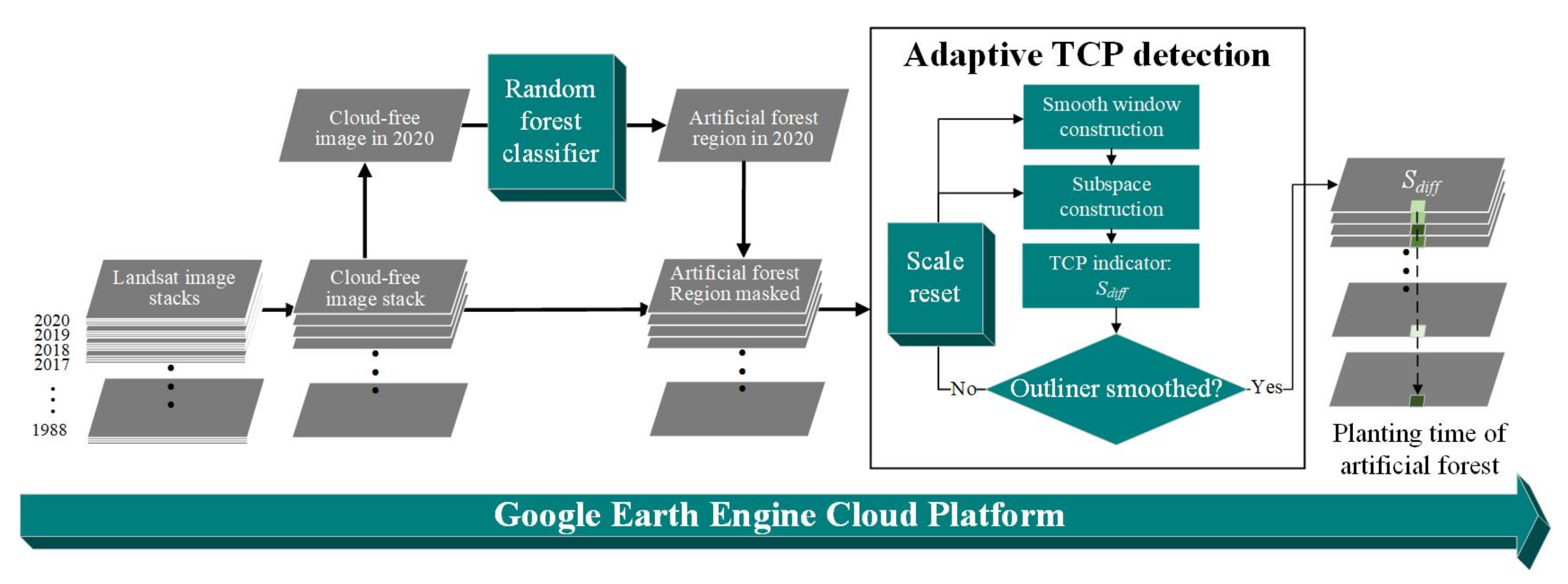
3.1. Artificial Forest Region Extraction

A variety of supervised classification methods have been integrated into the GEE platform, and the random forest (RF) classifier was selected here because of its wide application and reliable performance [40,41]. This method constructs multiple decision trees that depend on random vector values of independent sampling and classifies data through aggregation and guidance of decision trees [42], which is suitable for the high data dimensionality and multi-collinearity classification [43].
To perform this classification, 1840 land cover samples were collected through the high-resolution image from Google Earth and field survey, and the selection of those samples is based on the following two rules: First, the land cover type of each sample can be easily recognized in the Google Earth image; second, the pixels around the targeted sample have a similar land cover pattern. These samples include six categories: AF, cropland, sand, impervious surface, shrub, and water and the percentage of each category to the total samples is 20.93%, 16.69%, 14.62%, 19.29%, 14.67%, and 13.80%, respectively. Based on the unique features (spectral features and spectral indices) of each land cover type collected from those samples, a classification model was constructed with the RF classifier. Through times of tests, the classification accuracy reached the highest when the number of the decision tree was set to 110, and the number of the decision tree in the RF classifier was set to this value. After the classification, threefold cross-validation was implemented to evaluate the accuracy of the classification. The total training samples were divided into three parts, one of them was taken as validation samples each time and the other two parts were taken as training samples. The average value of the three times of classification accuracy was taken as the accuracy of the threefold cross-validation.

3.2. Afforestation Time Mapping

As indicated before, there is a significant increase in vegetation coverage represented by NDVI after afforestation in the sandy area, and the AF planting time can be captured by the abrupt change pattern that appears in the time-series NDVI curve. Because the NDVI images are only available since 1988, those AFs planted before 1988 are not considered in this study according to a threshold NDVI suggested by Anyamba and Tucker [44]. Therefore, when the NDVI value of any AF pixel in 1988 was higher than 0.2, it is thought that the AF was planted before 1988. After excluding the AFs planted before 1988, the planting times of other AF pixels were detected via the following two steps.

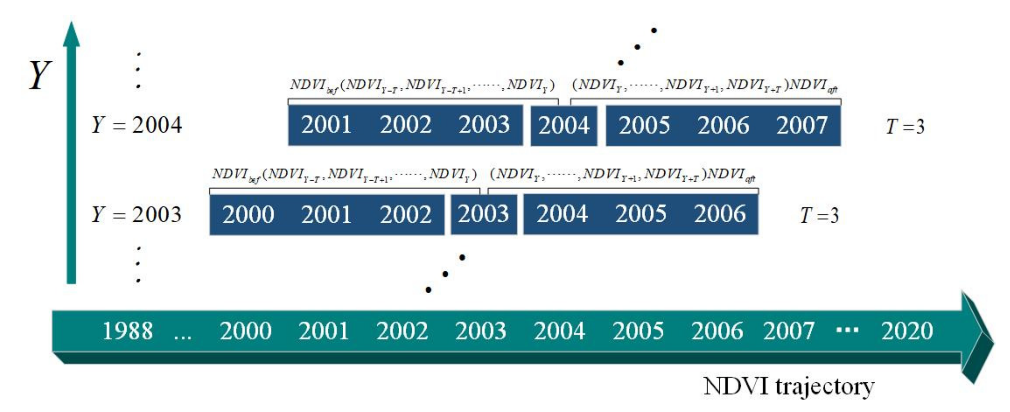
3.2.1. Subspace Construction

The developed algorithm for trend change detection includes six categories: threshold, difference, segmentation, trajectory classification, statistical boundary, and regression [45]. To represent the continuous trend around the probe point, a subspace segmentation was first set up to divide the NDVI trajectory into collections. The concept of the subspace in the change detection is to compare the subspaces in the trajectory between past and present and measure their dissimilarity by using a parameter to indicate the difference distance between them [18]. Figure 4 shows the sliding subspace with Y as the target year and T as the width of the subspace (take the width of three years as an example). Therefore, the time-series NDVIs from YT to Y made up the subspace before Y, and the NDVIs from Y to Y + T made up the subspace after Y. Probe point Y slides along the trajectory and the subspaces are fixed on both sides of the probe point and also slide along the trajectory.
In the subspace segmentation, the NDVI values obtained before and after the targeted year were needed for the study period 1988–2020. However, the NDVI values before 1988 or after 2020 are not available. Therefore, the NDVI values of 1998 and 2020 were replicated to the years before or after to meet the requirements of subspace construction. Taking 1988 as an example, the subspace after 1988 was available while the subspace before 1988 was nonexistent. Therefore, the NDVI value in 1988 was replicated to be the values of the previous years to reconstruct the subspace before 1988.

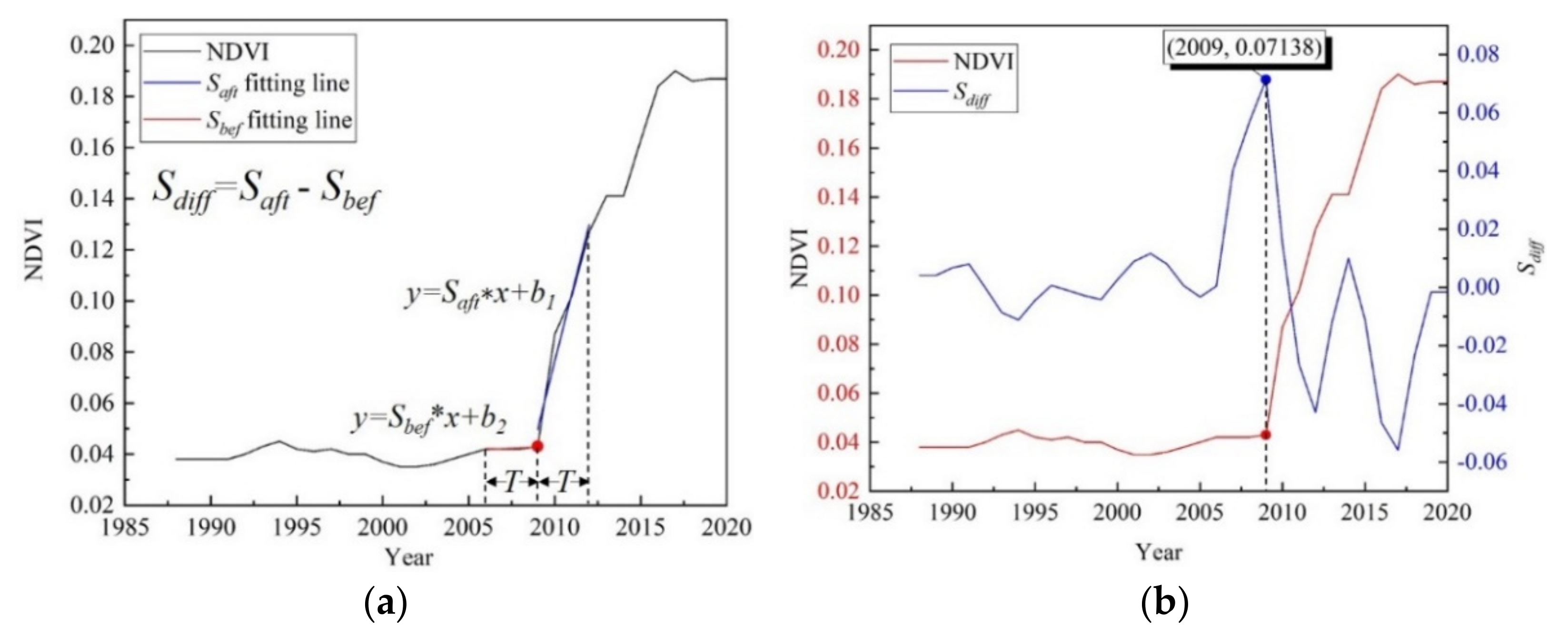
3.2.2. TCP Indicator Construction

After subspace segmentation, a linear fit was conducted for the NDVI values in both subspaces at each probe point to get the fitting line slopes. As shown in Figure 5a, the slopes of the left subspace (Sbef) and the right subspace (Saft) were calculated for probe point Y. Then, the difference between those two slopes (Sdiff) was used as an indicator to represent the variation of the curve; the indicator was inspired by Zuo, et al. [46].
Obviously, if there was an increasing trend at this point, Sdiff should have a positive value and vice versa. Meanwhile, the absolute value of Sdiff represents the degree of the abrupt changes, the larger it is the greater the degree of the abrupt change is. To demonstrate this fact, Figure 5b shows the original NDVI time-series curve in Figure 5a and the Sdiff curve derived with the subspace width of three years as an example. There is one year with the maximum Sdiff value in 2009 which is thought of as the AF planting time.

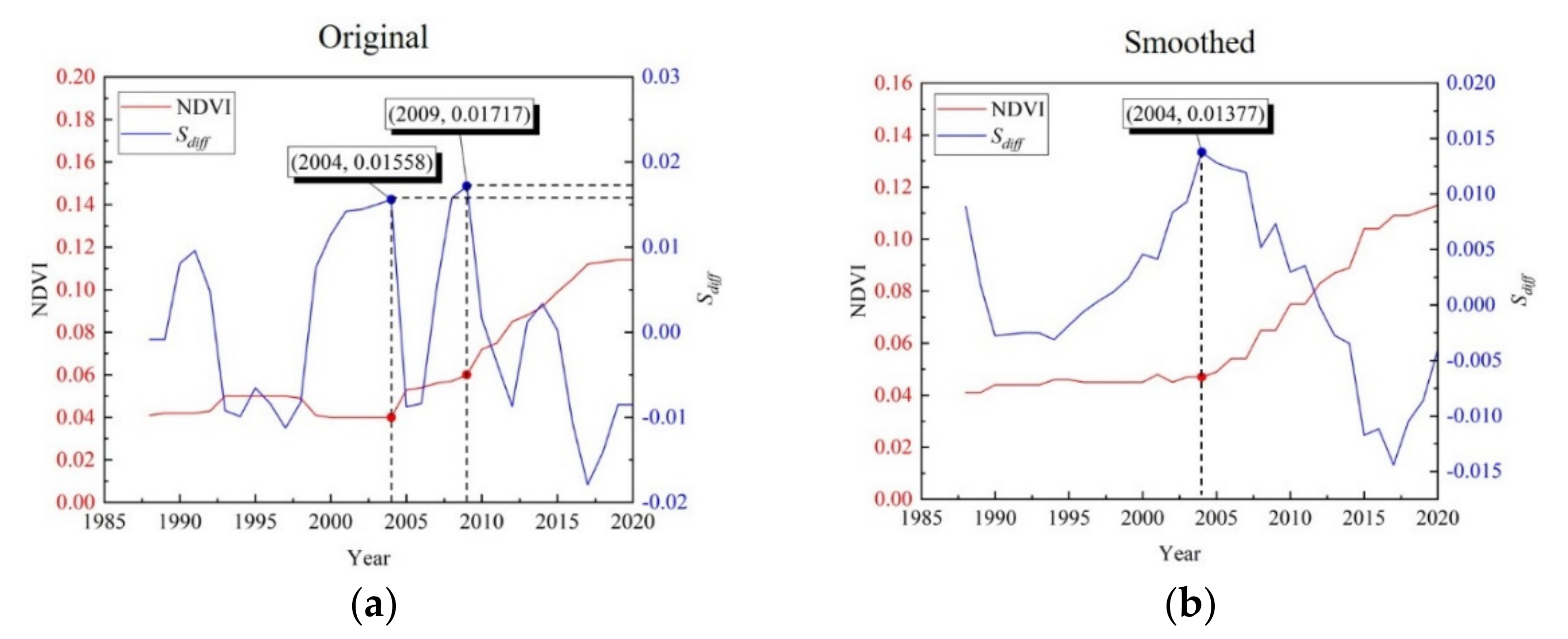
3.2.3. Adaptive TCP Detection

Ideally, the detection of the TCP can be simply determined according to the maximum value of Sdiff as shown in Figure 6. However, due to some uncertainties in the NDVI data caused by drought, plant diseases, insect pests, deforestation, inundation induced by temporary flood, and also the atmospheric effect on remote sensing data, there would be some outliers distorting the actual NDVI changing pattern. To reduce these influences and enhance the detection accuracy, a sliding window smooth method was applied to the NDVI trajectory before detection to smooth the abrupt changes induced by these uncertainties. Figure 6 shows a good example of outlier smoothing. Before smoothing, the actual TCP (2004) was not accurately detected according to the maximum value of Sdiff shown in Figure 6a. However, after smoothing (Figure 6b), the interference of the uncertainties in time-series NDVI was reduced and the expected TCP was accurately found.
Although the sliding window smoothing method can reduce the impacts from the uncertainties in the NDVI trajectory, how to determine the optimal width of the sliding window is important to effectively remove the disturbance from outliers. Therefore, an iteration detection scheme was implemented by changing the subspace width and the smoothing window size adaptively. Firstly, the initial subspace width was set to 2 and its maximum value was set to 5. The sliding window size was initialized at 2 with a maximum of 6. For each pixel which is hard to determine the dominated maximum Sdiff value, its subspace width was enlarged first to check the difference between the first two peak values of Sdiff. If the difference was still very small (the second biggest Sdiff is larger than 2/3 of the first biggest Sdiff), the subspace was enlarged again. Once the subspace extended to its maximum size, the smoothing window size was extended subsequently and the Sdiff series was generated again at different subspace sizes from 2 to 5. The iteration was stopped when the proportion of the second Sdiff peak value to the first peak value was no more than two-thirds. Finally, the TCP was set to the year of the maximum Sdiff.

4. Results

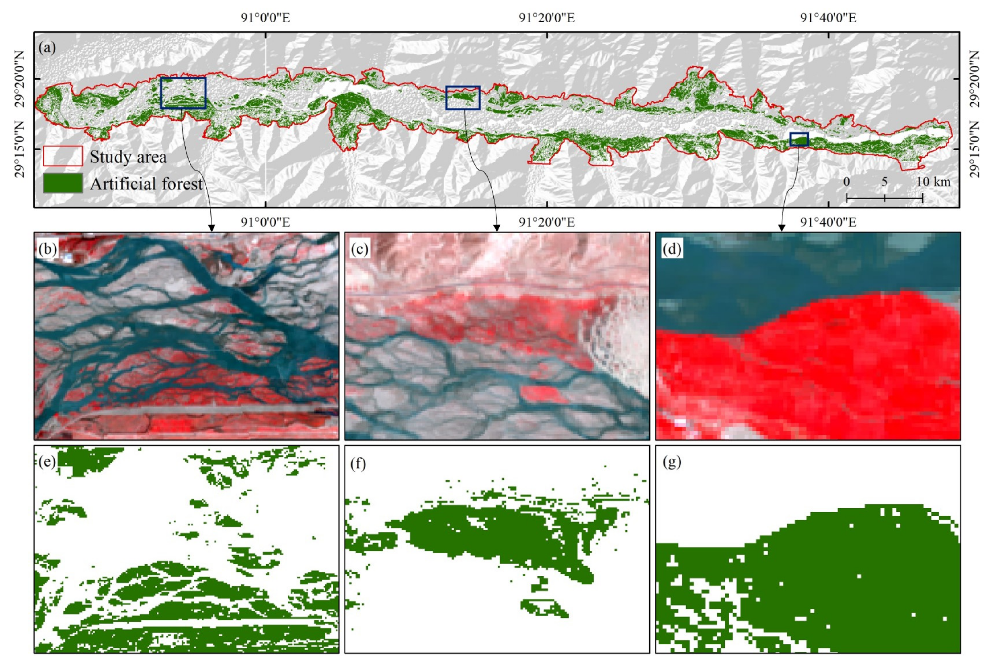
4.1. Artificial Forest Extraction Result

With the proposed classification method, the AF distribution of the study area was mapped as shown in Figure 7a. Threefold cross-validation was conducted for the classification results with an overall accuracy of 85.1% and a Kappa coefficient of 0.821. The main errors came from the misclassification among the vegetation surfaces likes AF, cropland, and shrubland. Especially for the newly planted forests, their poor vegetation coverage makes them similar to those of shrubs or crops. Clearly, the AFs are intensively distributed on the southern shore while the north shore has relatively few AFs. This difference was mainly attributed to the implementation of ecological engineering projects on the south shore in the early stage due to the widely distributed settlements. To better present the extraction accuracy, three plots were selected to show their original image and the extracted AF at each plot. Through visual comparison between the corresponding Landsat false-color images shown in Figure 7b–d and the AF extractions in Figure 7e–g, the extracted AFs have good spatial consistency with the real distribution.

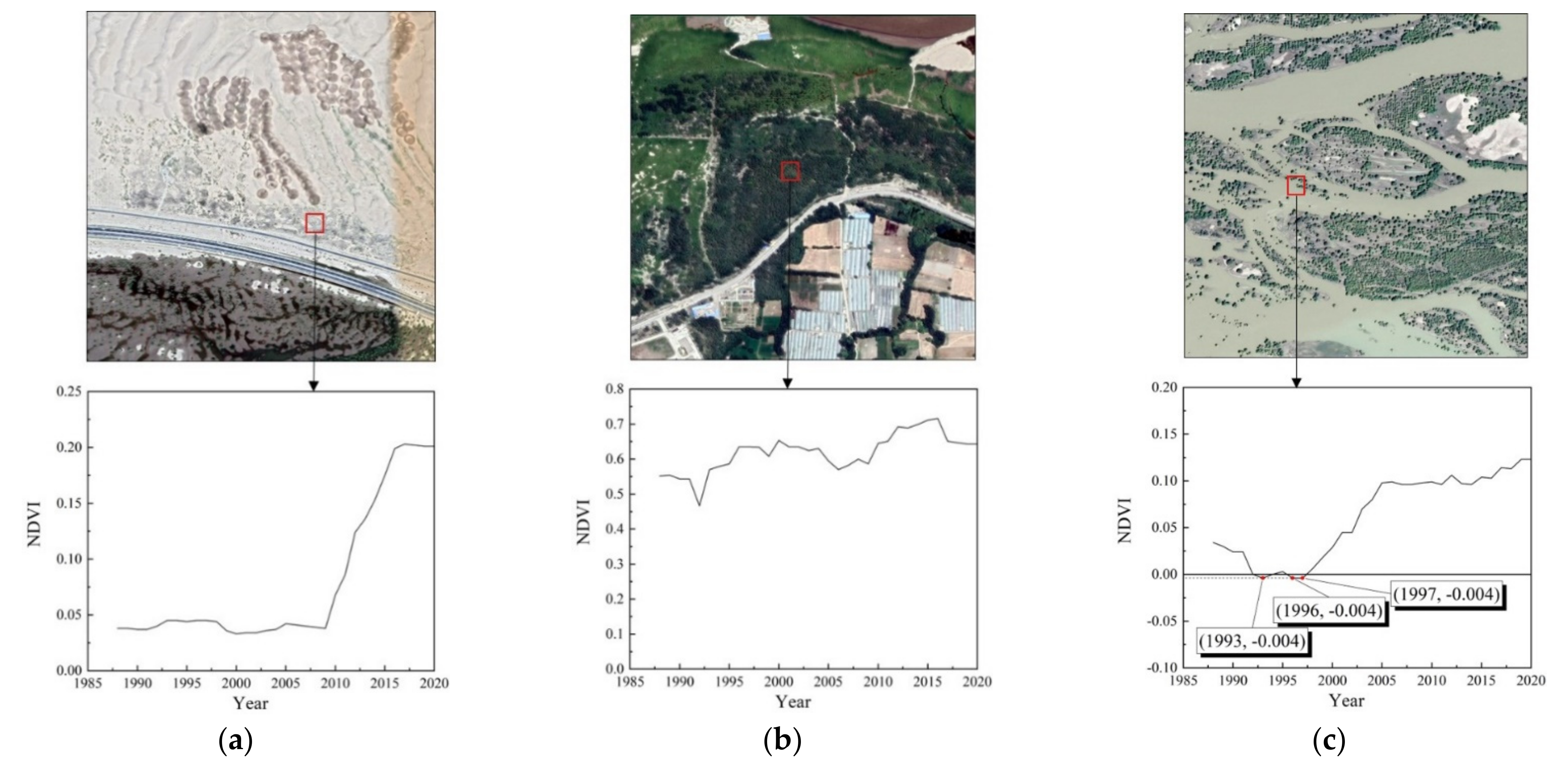
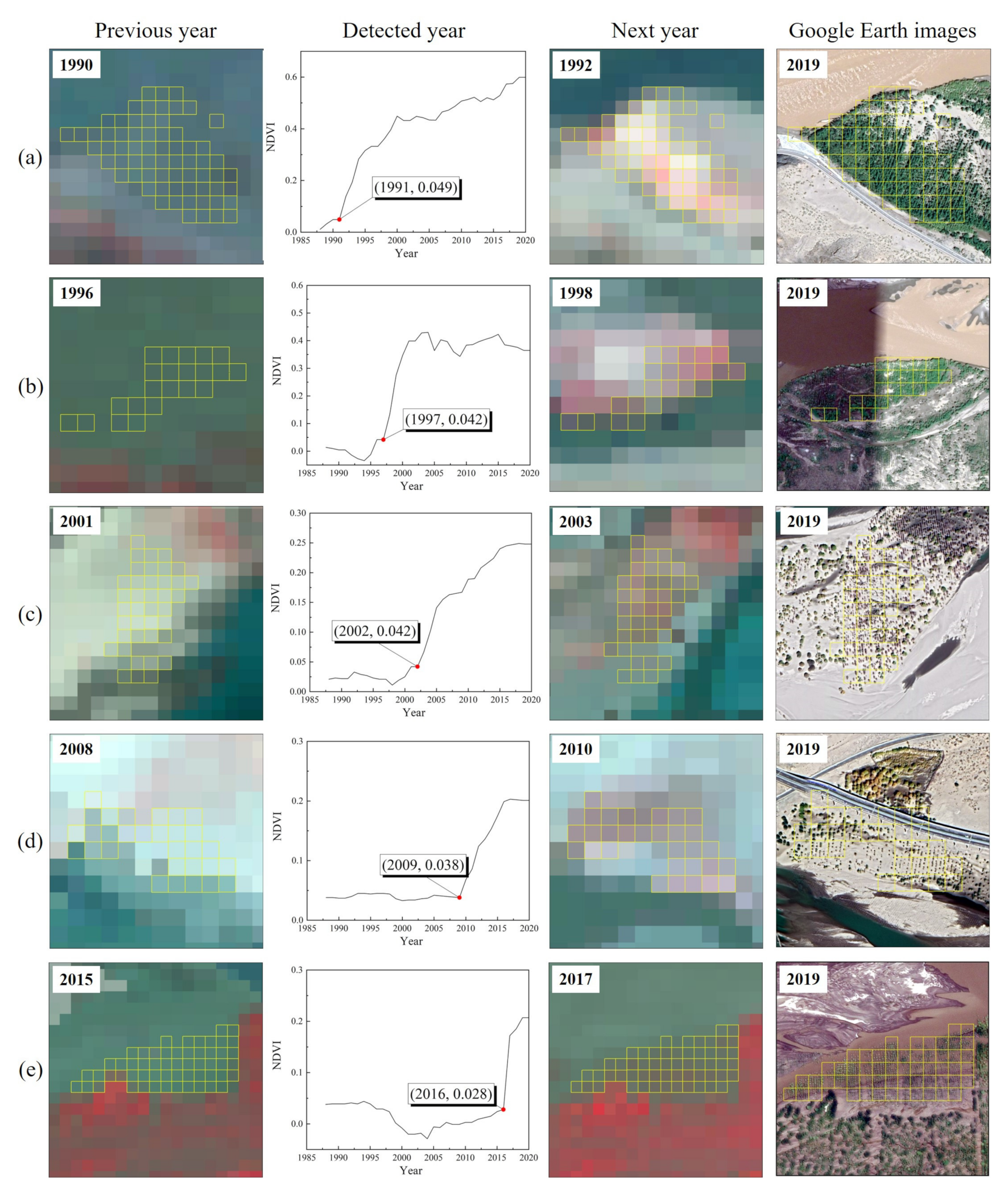
4.2. NDVI Series and the TCP Detections of Typical AF Samples

With the inspection of the NDVI trajectories of typical AFs, the NDVI series can be generally separated into three key types: ordinary AF, AF planted before 1988, and temporally inundated AF. Ordinary AFs are usually planted on barren surfaces or sandy surfaces to prevent desertification. Therefore, the NDVI curve has an obvious increase after AF plantation, and the NDVI value sticks to a relatively low level before AF planation, as shown in Figure 8a. The second type belongs to the AF patches with very good vegetation cover which were planted before 1988 (the earliest Landsat observable time). As shown in Figure 8b, their NDVI value always remains at a relatively high level and the variation is not as large as that of the ordinary AF. Therefore, the AF pixels with the mean NDVI in the initial three years bigger than a certain threshold (0.2 in this study) were considered to be planted in or before 1988. The third type was mainly distributed in the sandy islands of the riverbed, which was temporally inundated. As shown in Figure 8c, the temporal inundation introduced the mixed pixel effect with water and vegetation to reduce the NDVI values when compared with the values in non-inundated years.
To prove the reliability of representing the AF planting time by the TCP in time-series NDVI, Figure 9 shows the false-color images before and after the detected year, the NDVI trajectory, and the Google Earth image in 2019 of five AF samples. In the composite image, vegetation was shown as red color while water is dark blue and barren surface is yellow or white. The AF pixels were marked with yellow rectangles. Obviously, the AF pixels were water surfaces or sandy surfaces in the year before the detected year. After AF plantation, the pixels turn to light red, and this change can be reflected by the TCP detection shown in the NDVI trajectories. Therefore, the TCP of the time-series NDVI could represent the planting time of the AF by comparing the land cover changes in the afforestation area.

4.3. Afforestation Time Mapping and Validation

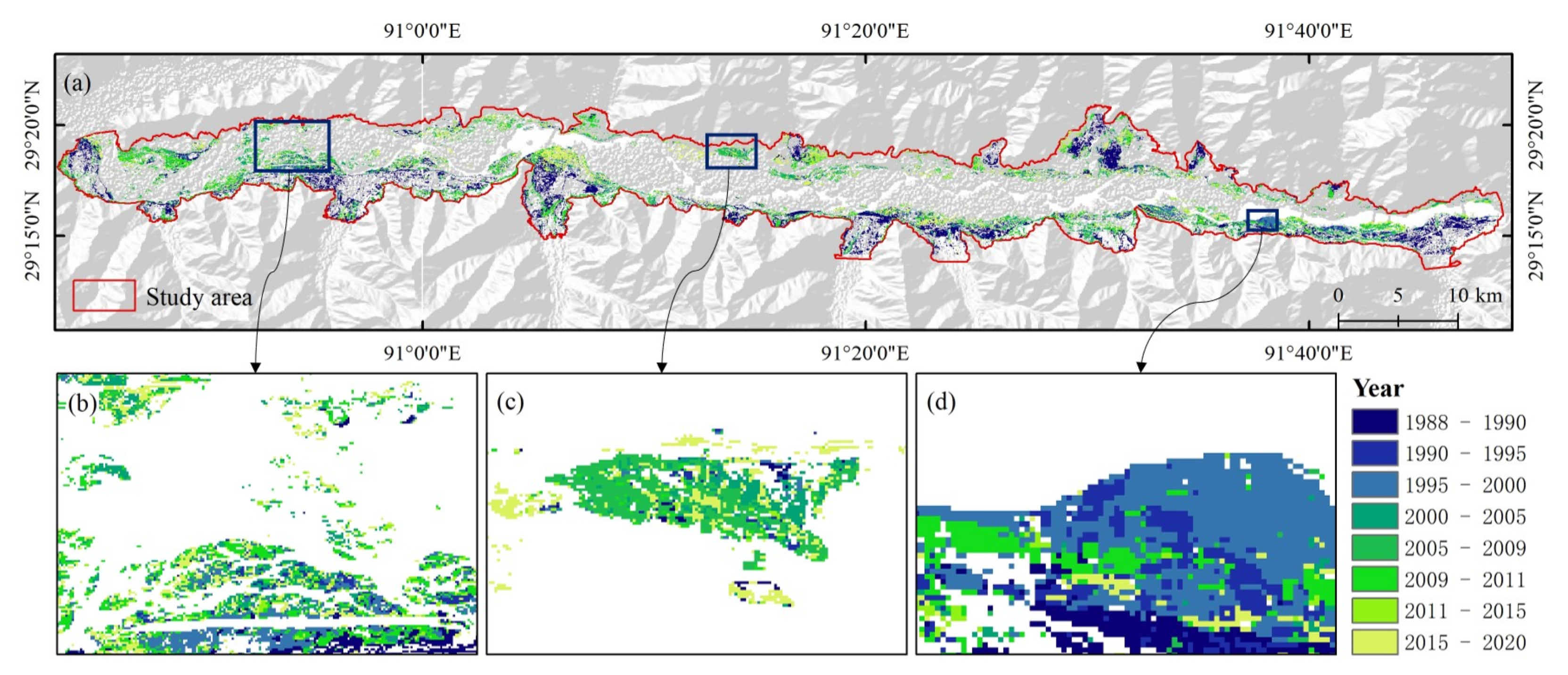
4.3.1. Afforestation Time Mapping Result

The proposed detection method was applied to the whole study area, and the mapping result of AF planting times is displayed in Figure 10a. The temporal-spatial distribution of AFs presents as regional clustering, which obeys the rule that AF plantation was always conducted from one region to another. Overall, the planting time of the south bank of the YZR was generally earlier than that of the north bank because prevention and control of desertification projects were mainly conducted at the south bank due to its widely distributed settlements. Take the three subregions in Figure 7 as examples, the AFs in Figure 10b were planted on the sandy island and strongly influenced by inundation. These pixels presented a patchy distribution which partly confirms the fact that AF planting was conducted at different times in different sized areas. In contrast, although there were also patches with different planting times, the planting times displayed in Figure 10c,d present clear temporal similarity for most of the AF pixels. In Figure 10c, the AF pixels close to the riverway (at the bottom) have an earlier planting time because of better water conditions than the pixels in the north. Similarly, the AF pixels in Figure 10d, in the south were first planted to protect the road, and then the AF plantation was conducted on the river shoal.

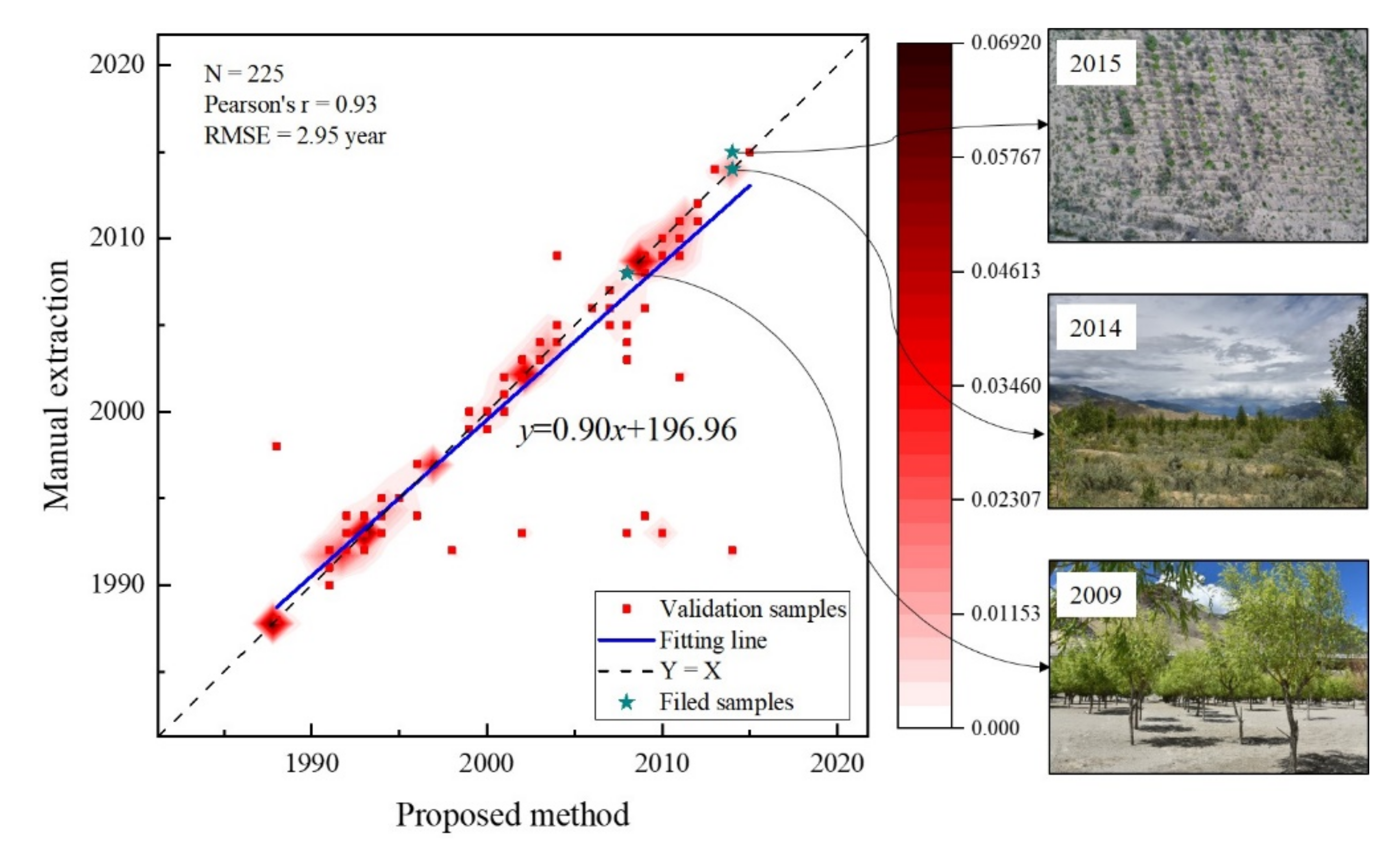
4.3.2. Validation with Field Samples

The detected AF planting time result was directly validated by the collected samples first. The result is shown in Figure 11. The density scatter plot shows good agreement between the detection results and the samples, with a Pearson correlation coefficient of 0.93 and a Root Mean Square Error (RMSE) of 2.95 years. Most of these points are well distributed around the 1:1 line. Meanwhile, the three AF field samples with true planting time also perform well in the consistency with the detected results. Two of them were consistent with the recorded planting time, while only one point has one year error. Meanwhile, there are also some points with big overestimation in the planting time and this may be attributed to the variation in vegetation cover induced by water inundation or deforestation.

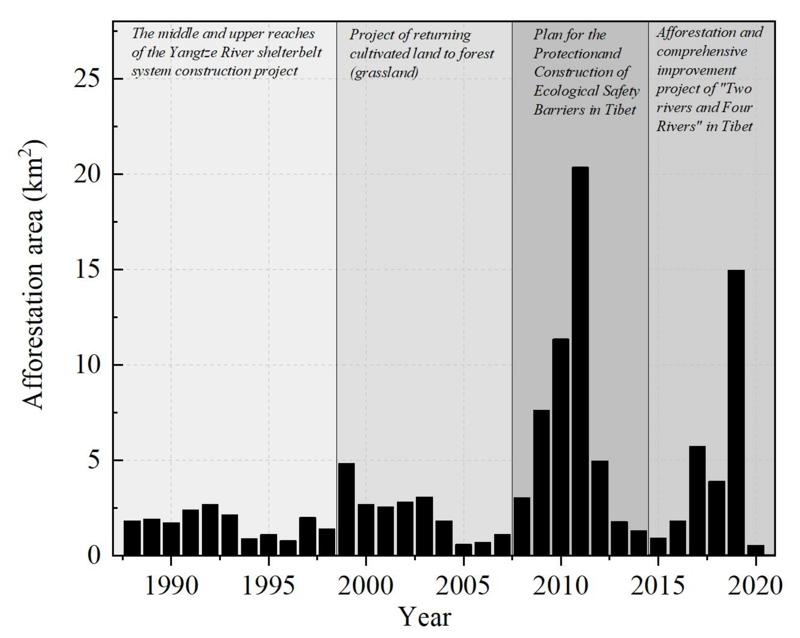
4.3.3. Temporal Consistency Analysis with Implementation of Ecological Projects

With the detection results, the temporal distribution of the AF planting time over the study area from 1988 to 2020 was investigated and shown in Figure 12. The observable time series can be divided into four phases according to the temporal pattern, which is highly consistent with the implementation of key ecological construction projects during this period.
In the early years (from 1988 to 1998), the afforestation area in each year always keeps to a low level, because the afforestation was mainly conducted voluntarily by civilians around the settlements and there is small input from local or central government. It can be referred from the report from this website http://www.seac.gov.cn/seac/xwzx/200303/1010522.shtml, accessed on 25 November 2021. From 1999 to 2007, the afforestation area has slight increases because of the project of returning cultivated land to forest (grassland). However, the government mainly focused on the afforestation along the roads and railways, which occupy a small area in this region.
In the following years (from 2008 to 2014), the afforestation area had a fast increase because of the conduction of the Plan for the Protection and Construction of Ecological Safety Barriers in Tibet, and the central government invested 8.35 billion yuan to protect and restore the key ecological function zones in the Tibetan Plateau (http://www.scio.gov.cn/zfbps/32832/Document/1633895/1633895.htm, accessed on 25 November 2021). In recent years (from 2015 to 2020), the project for the protection and construction of an eco-safety barrier (around 10.7 billion investments) assists the afforestation in the basins of the Yarlung Zangbo, Nujiang, Lhasa, Nyangchu, Yalong, and Shiquan Rivers. Therefore, the afforestation area continues to be at a high level in this region. Obviously, the temporal consistency between the temporal pattern of the AF planting time and the implementation of key ecological projects in this region confirms the reliability of the detection results.

5. Discussion

Many algorithms have been proven to perform well in forest change mapping. However, not all of them are suitable to detect the planting time of the AFs. The afforestation generated continuous trend changes with a smaller degree than that of the outliers and the purpose of this study focuses on extracting the AF planting time from the disturbance of outliers. In this study, trend, difference, and segmentation were combined to carry out continuous trend change detection, and the adaptive scale selection was imported to reduce the influence of outliers. In relative studies, Liu, et al. [47] mapped the afforestation and deforestation using the IFZ index proposed in VCT [31] which has proven to perform well in forest disturbance detection, and the planting time was detected by the threshold of the IFZ. However, because of high spatial-temporal heterogeneity and external factors, there may be some outliers with different change degrees, distorting the planting time detection. Consequently, the threshold is different due to different afforestation ground conditions, such as sandy land, grassland, and shrubs, which may be confused by the condition of cropland. Therefore, the results using thresholds judgment may be confused by different environmental conditions in large-scale spatial-temporal distribution planting time mapping, and this error can be avoided by focusing on the trend change characteristic in the time-series vegetation index.
However, it is difficult to avoid the disturbance of the outliers during change detection. Spatial heterogeneity results in different NDVI value ranges during afforestation, and the use of threshold is always controversial, such as the TVCMA taking thresholds as change detection elements. The trend in the change detection can represent an overall tendency of a phenomenon and reduce the impact of individual outliers [48], while the use of single-point data is not enough to express the continuous trend change characteristic and is susceptible to outliers. Meanwhile, for local analysis to extract the trend features from the NDVI trajectory, the subspace was used for segmentation. Moreover, the indicator Sdiff was introduced to indicate the continuous trend change around the probe point. For the continuous construction of ecological engineering, the TCP (AF planting time) can exist at any time in the time series and produce a different mean square error (MSE) during the total least square fitting in LandTrendr, which may be confused by the MSE of outliers. Thus, the adaptive selection of the window size and the subspace size was imported to reduce the influence of outliers. Finally, aiming at the characteristics of the AF temporal vegetation index, combining the three elements minimizes the impact of outliers while expressing the trend change characteristic.
The detection results obtained in this study proved that the proposed change detection is suitable for extracting the TCP in time-series vegetation index curve which is firmly connected to the AF planting time by finding the characteristic within dense image stacks. In contrast to land cover change analysis of images from certain time points, such as the land cover mapping with images every five years or just two images at different times for analysis [49,50], the use of time-series images from each year covered the changing information with higher temporal resolution. Meanwhile, the powerful computing capability of the GEE platform greatly improved the efficiency of dense image series analysis, there are similar investigations based on GEE in the field of agriculture [51], population [52], vegetation [53], and surface water [54].
With the above basic structures and platform, the adaptive segmentation and smooth in this method shows good accuracy in finding the right TCP by automatically selecting the suitable scale of the smoothing window and segmentation subspace for each pixel, which helps remove the impact of outliers. Because changes at different degrees require different scales of window smooth and subspace segmentation, the oversize of the smoothing window will miss the exact detection of the real TCP, while the smaller size cannot remove the disturbance of outliers. Therefore, the adaptive scale selection introduced in this study alleviates this impact. Taking a sample pixel as an example (Figure 13), the Sdiff of an outlier in 2009 was smoothed after the width of the smoothing window increased and the TCP remain unchanged. Through a wider smoothing window, the change degree at a smaller scale was reduced and the smoothed curve provided a better description of the changes in the NDVI trajectory than the initial curve. In other words, the use of smoothing windows at different scales produces different smoothing effects, which means that a single scale of the smoothing window is not suitable for each pixel to remove the disturbance.
The proposed TCP detection method shows high resistance to disturbances through adaptive changes in the window width and the length of the subspace. However, for some cases when there are some significant disturbances after AF planting, such as deforestation, the NDVI trajectory does not display a continuously increasing trend but is mixed with some declining periods or a sudden increase as shown in Figure 14, which generates a larger Sdiff during the growth stage than that of the planting time. The increasing stage after this disturbance distorts the TCP detection results and introduces errors in the results. Therefore, it is necessary to combine other quantitative indicators to constrain the detected time and stick to a low biomass level to reduce the impact caused by natural or human factors during the growing stage.
In addition to the uncertainty related to the disturbances, the uncertainty associated with AF extraction is another factor that should be considered. The wide distribution of planting time and different growth stages of the AF make the AF information easily confused with the spectral pattern of the cropland and shrubland. Due to the unique texture of AF planting, texture extraction [55,56] is a widely used method for extracting AF areas in remote sensing. However, the spatial resolution of the Landsat image is not sufficiently high for AF texture analysis. Therefore, there is still space to improve the AF extraction accuracy. Inclusion of the texture information from higher resolution image data, such as the Unmanned Aerial Vehicle (UAV) based Remote Sensing images, and classification at the patch level will partly assist the further improvement of AF planting time mapping.

6. Conclusions

In this study, an adaptive detection algorithm for identifying the planting times of AFs was proposed based on the time-series NDVI values acquired from the Google Earth Engine platform. With this method, an AF planting time map was generated for the middle section of the YZR, the AF extraction from RF classification with an overall accuracy of 85.1%, and a Kappa coefficient of 0.821. The validation of the detected planting time with samples collected in this region indicates the good performance of the proposed method with a Pearson correlation coefficient of 0.93 and an RMSE of 2.95 years. The results showed that the AFs planted in the early years were mainly distributed in the southern shore of the YZR, and the AFs of recent decades occupied a large area especially the AFs planted from 2008 to 2014, and another peak existed in 2019, which presented good consistency with the implementation time of the eco-reconstruction projects in this region.
In general, the self-adaptive process in the proposed method reduced the impacts of disturbances induced by outliers effectively. Meanwhile, the confusion with the real planting time caused by different afforestation conditions was reduced by focusing on the trend change characteristic in time-series NDVI. This study provides an important insight into the spatial and temporal distribution of AF along the YZR valley, which is very important for further assessing ecological projects and evaluating their functions in controlling widespread desertification. According to this data, the environmental changes of AFs areas with different spatial-temporal distributions can be used to quantify the role of afforestation in resisting desertification.

Author Contributions

Conceptualization, W.Z. and H.F.; methodology, H.F. and W.Z.; software, H.F., Q.Z. and M.Y.; validation, H.F., Q.Z., M.Y. and W.Z.; investigation, H.F., Q.Z., M.Y. and W.Z.; resources, W.Z. and D.X.; data curation, H.F.; writing—original draft preparation, H.F. and W.Z.; writing—review and editing, W.Z. and H.F.; visualization, H.F., Q.Z. and M.Y.; supervision, W.Z., D.X. and D.Y.; project administration, W.Z.; funding acquisition, W.Z., D.X. and D.Y. All authors have read and agreed to the published version of the manuscript.

Funding

This research was funded partially by the Second Tibetan Plateau Scientific Expedition and Research Program (STEP) (2019QZKK0404), the National Natural Science Foundation of China (Grant No. 42071349), the Sichuan Science and Technology Program (2020JDJQ0003), and the CAS “Light of West China” Program.

Institutional Review Board Statement

Not applicable.

Informed Consent Statement

Not applicable.

Data Availability Statement

The Landsat Surface Reflectance product used in this study is available on the Google Earth Engine platform.

Acknowledgments

We would thank the three reviewers for their valuable and constructive comments and suggestions which help a lot for improving the quality of this study. Meanwhile, we would express our gratitude to the Google Earth Engine platform for supplying Landsat data and image processing.

Conflicts of Interest

The authors declare no conflict of interest.

References

  1. Liu, Z.; Yao, Z.; Huang, H.; Wu, S.; Liu, G. Land Use And Climate Changes And Their Impacts on Runoff In the Yarlung Zangbo River Basin, China. Land Degrad. Dev. 2014, 25, 203–215. [Google Scholar] [CrossRef]
  2. Zhou, N.; Li, Q.; Zhang, C.-L.; Chi-Hua, H.; Wu, Y.; Zhu, B.; Cen, S.; Huang, X. Grain size characteristics of aeolian sands and their implications for the aeolian dynamics of dunefields within a river valley on the southern Tibet Plateau: A case study from the Yarlung Zangbo river valley. Catena 2021, 196, 104794. [Google Scholar] [CrossRef]
  3. Zhang, C.-L.; Li, Q.; Shen, Y.-P.; Zhou, N.; Wang, X.-S.; Li, J.; Jia, W.-R. Monitoring of aeolian desertification on the Qinghai-Tibet Plateau from the 1970s to 2015 using Landsat images. Sci. Total Environ. 2018, 619–620, 1648–1659. [Google Scholar] [CrossRef]
  4. Liu, Y.; Wang, Y.-S.; Shen, T. Spatial distribution and formation mechanism of aeolian sand in the middle reaches of the Yarlung Zangbo River. J. Mt. Sci. 2019, 16, 1987–2000. [Google Scholar] [CrossRef]
  5. Wu, Y. The Study on the Relationship between Ecological Conservation and Rural Households’ Income Improvement in Tibet. Ph.D. Thesis, Beijing Forestry University, Beijing, China, 2016. [Google Scholar]
  6. Richter, D.D.; Markewitz, D.; Trumbore, S.E.; Wells, C.G. Rapid accumulation and turnover of soil carbon in a re-establishing forest. Nature 1999, 400, 56–58. [Google Scholar] [CrossRef] [Green Version]
  7. Cui, G.-S.; Zhang, L.; Shen, W.; Liu, X.-S.; Wang, Y.-T. Biomass allocation and carbon density of Sophora moorcroftiana shrublands in the middle reaches of Yarlung Zangbo River, Xizang, China. Chin. J. Plant Ecol. 2017, 41, 53. [Google Scholar]
  8. Chen, J.M. Carbon neutrality: Toward a sustainable future. Innovation 2021, 2, 100127. [Google Scholar] [CrossRef]
  9. Ma, Q.; Fehmi, J.S.; Zhang, D.; Fan, B.; Chen, F. Changes in wind erosion over a 25-year restoration chronosequence on the south edge of the Tengger Desert, China: Implications for preventing desertification. Environ. Monit. Assess. 2017, 189, 463. [Google Scholar] [CrossRef] [Green Version]
  10. Su, Y.Z.; Zhao, W.Z.; Su, P.X.; Zhang, Z.H.; Wang, T.; Ram, R. Ecological effects of desertification control and desertified land reclamation in an oasis–desert ecotone in an arid region: A case study in Hexi Corridor, northwest China. Ecol. Eng. 2007, 29, 117–124. [Google Scholar] [CrossRef]
  11. Tao, W. Progress in sandy desertification research of China. J. Geogr. Sci. 2004, 14, 387–400. [Google Scholar] [CrossRef]
  12. Zhao, C.; Zhang, H.; Song, C.; Zhu, J.-K.; Shabala, S. Mechanisms of Plant Responses and Adaptation to Soil Salinity. Innovation 2020, 1, 100017. [Google Scholar] [CrossRef] [PubMed]
  13. Yang, M.; Zhao, W.; Zhan, Q.; Xiong, D. Spatiotemporal Patterns of Land Surface Temperature Change in the Tibetan Plateau Based on MODIS/Terra Daily Product From 2000 to 2018. IEEE J. Sel. Top. Appl. Earth Obs. Remote. Sens. 2021, 14, 6501–6514. [Google Scholar] [CrossRef]
  14. Doelman, J.C.; Stehfest, E.; van Vuuren, D.P.; Tabeau, A.; Hof, A.F.; Braakhekke, M.C.; Gernaat, D.E.H.J.; van den Berg, M.; van Zeist, W.-J.; Daioglou, V.; et al. Afforestation for climate change mitigation: Potentials, risks and trade-offs. Glob. Chang. Biol. 2020, 26, 1576–1591. [Google Scholar] [CrossRef] [PubMed]
  15. Wardle, D.A.; Bonner, K.I.; Barker, G.M.; Yeates, G.W.; Nicholson, K.S.; Bardgett, R.D.; Watson, R.N.; Ghani, A. Plant Removals in Perennial Grassland: Vegetation Dynamics, Decomposers, Soil Biodiversity, and Ecosystem Properties. Ecol. Monogr. 1999, 69, 535–568. [Google Scholar] [CrossRef]
  16. Li, X.-R.; Zhang, J.-G.; Liu, L.-C.; Chen, H.-S.; Shi, Q.-H. Plant Diversity and Succession of Artificial Vegetation Types and Environment in an Arid Desert Region of China. In Conserving Biodiversity in Arid Regions: Best Practices in Developing Nations; Lemons, J., Victor, R., Schaffer, D., Eds.; Springer: Boston, MA, USA, 2003; pp. 179–188. [Google Scholar]
  17. Chen, S. Eco-Benefit of Ecoloigical Restoration and Reconstruction in Mining Area-Case Study of Phosphorite in Kunyang, Yunnan Province. Master’s Thesis, Kunming University of Science and Technology, Kunming, China, 2009. [Google Scholar]
  18. Liu, S.; Yamada, M.; Collier, N.; Sugiyama, M. Change-point detection in time-series data by relative density-ratio estimation. Neural Netw. 2013, 43, 72–83. [Google Scholar] [CrossRef] [PubMed] [Green Version]
  19. Xie, G.; Li, J.-F.; Wang, S.-Q.; Yao, Y.-F.; Sun, B.; Ferguson, D.K.; Li, C.-S.; Deng, T.; Liu, X.-D.; Wang, Y.-F. Bridging the knowledge gap on the evolution of the Asian monsoon during 26–16 Ma. Innovation 2021, 2, 100110. [Google Scholar] [CrossRef]
  20. Chen, F.; Zhang, J.; Liu, J.; Cao, X.; Hou, J.; Zhu, L.; Xu, X.; Liu, X.; Wang, M.; Wu, D.; et al. Climate change, vegetation history, and landscape responses on the Tibetan Plateau during the Holocene: A comprehensive review. Quat. Sci. Rev. 2020, 243, 106444. [Google Scholar] [CrossRef]
  21. Wulder, M.A.; White, J.C.; Loveland, T.R.; Woodcock, C.E.; Belward, A.S.; Cohen, W.B.; Fosnight, E.A.; Shaw, J.; Masek, J.G.; Roy, D.P. The global Landsat archive: Status, consolidation, and direction. Remote. Sens. Environ. 2016, 185, 271–283. [Google Scholar] [CrossRef] [Green Version]
  22. Loveland, T.R.; Dwyer, J.L. Landsat: Building a strong future. Remote Sens. Environ. 2012, 122, 22–29. [Google Scholar] [CrossRef]
  23. Moon, M.; Zhang, X.; Henebry, G.M.; Liu, L.; Gray, J.M.; Melaas, E.K.; Friedl, M.A. Long-term continuity in land surface phenology measurements: A comparative assessment of the MODIS land cover dynamics and VIIRS land surface phenology products. Remote Sens. Environ. 2019, 226, 74–92. [Google Scholar] [CrossRef]
  24. Cho, M.A.; Ramoelo, A. Optimal dates for assessing long-term changes in tree-cover in the semi-arid biomes of South Africa using MODIS NDVI time series (2001–2018). Int. J. Appl. Earth Obs. Geoinf. 2019, 81, 27–36. [Google Scholar] [CrossRef]
  25. Zhao, W.; He, J.; Yin, G.; Wen, F.; Wu, H. Spatiotemporal Variability in Land Surface Temperature Over the Mountainous Region Affected by the 2008 Wenchuan Earthquake from 2000 to 2017. J. Geophys. Res.-Atmos. 2019, 124, 1975–1991. [Google Scholar] [CrossRef]
  26. Dorren, L.K.A.; Maier, B.; Seijmonsbergen, A.C. Improved Landsat-based forest mapping in steep mountainous terrain using object-based classification. For. Ecol. Manag. 2003, 183, 31–46. [Google Scholar] [CrossRef]
  27. Coppin, P.R.; Bauer, M.E. Digital change detection in forest ecosystems with remote sensing imagery. Remote. Sens. Rev. 1996, 13, 207–234. [Google Scholar] [CrossRef]
  28. Pause, M.; Schweitzer, C.; Rosenthal, M.; Keuck, V.; Bumberger, J.; Dietrich, P.; Heurich, M.; Jung, A.; Lausch, A. In Situ/Remote Sensing Integration to Assess Forest Health—A Review. Remote. Sens. 2016, 8, 471. [Google Scholar] [CrossRef] [Green Version]
  29. Kennedy, R.E.; Cohen, W.B.; Schroeder, T.A. Trajectory-based change detection for automated characterization of forest disturbance dynamics. Remote. Sens. Environ. 2007, 110, 370–386. [Google Scholar] [CrossRef]
  30. Fensholt, R.; Rasmussen, K.; Nielsen, T.T.; Mbow, C. Evaluation of earth observation based long term vegetation trends—Intercomparing NDVI time series trend analysis consistency of Sahel from AVHRR GIMMS, Terra MODIS and SPOT VGT data. Remote Sens. Environ. 2009, 113, 1886–1898. [Google Scholar] [CrossRef]
  31. Huang, C.; Goward, S.N.; Masek, J.G.; Thomas, N.; Zhu, Z.; Vogelmann, J.E. An automated approach for reconstructing recent forest disturbance history using dense Landsat time series stacks. Remote. Sens. Environ. 2010, 114, 183–198. [Google Scholar] [CrossRef]
  32. Ochtyra, A.; Marcinkowska-Ochtyra, A.; Raczko, E. Threshold- and trend-based vegetation change monitoring algorithm based on the inter-annual multi-temporal normalized difference moisture index series: A case study of the Tatra Mountains. Remote. Sens. Environ. 2020, 249, 112026. [Google Scholar] [CrossRef]
  33. Yang, Y.; Luo, J.; Huang, Q.; Wu, W.; Sun, Y. Weighted Double-Logistic Function Fitting Method for Reconstructing the High-Quality Sentinel-2 NDVI Time Series Data Set. Remote. Sens. 2019, 11, 2342. [Google Scholar] [CrossRef] [Green Version]
  34. Zhan, Q.; Zhao, W.; Yang, M.; Xiong, D. A long-term record (1995–2019) of the dynamics of land desertification in the middle reaches of Yarlung Zangbo River basin derived from Landsat data. Geogr. Sustain. 2021, 2, 12–21. [Google Scholar] [CrossRef]
  35. Pan, L.; Xia, H.; Zhao, X.; Guo, Y.; Qin, Y. Mapping Winter Crops Using a Phenology Algorithm, Time-Series Sentinel-2 and Landsat-7/8 Images, and Google Earth Engine. Remote. Sens. 2021, 13, 2510. [Google Scholar] [CrossRef]
  36. Zuo, D.; Han, Y.; Xu, Z.; Li, P.; Ban, C.; Sun, W.; Pang, B.; Peng, D.; Kan, G.; Zhang, R.; et al. Time-lag effects of climatic change and drought on vegetation dynamics in an alpine river basin of the Tibet Plateau, China. J. Hydrol. 2021, 600, 126532. [Google Scholar] [CrossRef]
  37. Pan, L.; Xia, H.; Yang, J.; Niu, W.; Wang, R.; Song, H.; Guo, Y.; Qin, Y. Mapping cropping intensity in Huaihe basin using phenology algorithm, all Sentinel-2 and Landsat images in Google Earth Engine. Int. J. Appl. Earth Obs. Geoinf. 2021, 102, 102376. [Google Scholar] [CrossRef]
  38. Foga, S.; Scaramuzza, P.L.; Guo, S.; Zhu, Z.; Dilley, R.D.; Beckmann, T.; Schmidt, G.L.; Dwyer, J.L.; Joseph Hughes, M.; Laue, B. Cloud detection algorithm comparison and validation for operational Landsat data products. Remote. Sens. Environ. 2017, 194, 379–390. [Google Scholar] [CrossRef] [Green Version]
  39. Roy, D.P.; Kovalskyy, V.; Zhang, H.K.; Vermote, E.F.; Yan, L.; Kumar, S.S.; Egorov, A. Characterization of Landsat-7 to Landsat-8 reflective wavelength and normalized difference vegetation index continuity. Remote. Sens. Environ. 2016, 185, 57–70. [Google Scholar] [CrossRef] [Green Version]
  40. Pal, M. Random forest classifier for remote sensing classification. Int. J. Remote. Sens. 2005, 26, 217–222. [Google Scholar] [CrossRef]
  41. Phan, T.N.; Kuch, V.; Lehnert, L.W. Land Cover Classification using Google Earth Engine and Random Forest Classifier—The Role of Image Composition. Remote. Sens. 2020, 12, 2411. [Google Scholar] [CrossRef]
  42. Breiman, L. Random forests. Mach. Learn. 2001, 45, 5–32. [Google Scholar] [CrossRef] [Green Version]
  43. Belgiu, M.; Drăguţ, L. Random forest in remote sensing: A review of applications and future directions. ISPRS J. Photogramm. Remote. Sens. 2016, 114, 24–31. [Google Scholar] [CrossRef]
  44. Anyamba, A.; Tucker, C.J. Analysis of Sahelian vegetation dynamics using NOAA-AVHRR NDVI data from 1981–2003. J. Arid. Environ. 2005, 63, 596–614. [Google Scholar] [CrossRef]
  45. Zhu, Z. Change detection using landsat time series: A review of frequencies, preprocessing, algorithms, and applications. ISPRS J. Photogramm. Remote. Sens. 2017, 130, 370–384. [Google Scholar] [CrossRef]
  46. Zuo, B.; Li, J.; Sun, C.; Zhou, X. A new statistical method for detecting trend turning. Theor. Appl. Climatol. 2019, 138, 201–213. [Google Scholar] [CrossRef] [Green Version]
  47. Liu, L.; Tang, H.; Caccetta, P.; Lehmann, E.A.; Hu, Y.; Wu, X. Mapping afforestation and deforestation from 1974 to 2012 using Landsat time-series stacks in Yulin District, a key region of the Three-North Shelter region, China. Environ. Monit. Assess. 2013, 185, 9949–9965. [Google Scholar] [CrossRef]
  48. Cao, Y.; Xie, Y.; Gebraeel, N. Multi-sensor slope change detection. Ann. Oper. Res. 2018, 263, 163–189. [Google Scholar] [CrossRef] [Green Version]
  49. Singh, A. Review Article Digital change detection techniques using remotely-sensed data. Int. J. Remote. Sens. 1989, 10, 989–1003. [Google Scholar] [CrossRef] [Green Version]
  50. Coppin, P.; Jonckheere, I.; Nackaerts, K.; Muys, B.; Lambin, E. Review ArticleDigital change detection methods in ecosystem monitoring: A review. Int. J. Remote. Sens. 2004, 25, 1565–1596. [Google Scholar] [CrossRef]
  51. Shelestov, A.; Lavreniuk, M.; Kussul, N.; Novikov, A.; Skakun, S. Large scale crop classification using Google earth engine platform. In Proceedings of the 2017 IEEE International Geoscience and Remote Sensing Symposium (IGARSS), Fort Worth, TX, USA, 23–28 July 2017; pp. 3696–3699. [Google Scholar]
  52. Patel, N.N.; Angiuli, E.; Gamba, P.; Gaughan, A.; Lisini, G.; Stevens, F.R.; Tatem, A.J.; Trianni, G. Multitemporal settlement and population mapping from Landsat using Google Earth Engine. Int. J. Appl. Earth Obs. Geoinf. 2015, 35, 199–208. [Google Scholar] [CrossRef] [Green Version]
  53. Kennedy, R.E.; Yang, Z.; Gorelick, N.; Braaten, J.; Cavalcante, L.; Cohen, W.B.; Healey, S. Implementation of the LandTrendr Algorithm on Google Earth Engine. Remote. Sens. 2018, 10, 691. [Google Scholar] [CrossRef] [Green Version]
  54. Wang, C.; Jia, M.; Chen, N.; Wang, W. Long-Term Surface Water Dynamics Analysis Based on Landsat Imagery and the Google Earth Engine Platform: A Case Study in the Middle Yangtze River Basin. Remote. Sens. 2018, 10, 1635. [Google Scholar] [CrossRef] [Green Version]
  55. Akar, Ö.; Güngör, O. Integrating multiple texture methods and NDVI to the Random Forest classification algorithm to detect tea and hazelnut plantation areas in northeast Turkey. Int. J. Remote. Sens. 2015, 36, 442–464. [Google Scholar] [CrossRef]
  56. Gebreslasie, M.T.; Ahmed, F.B.; van Aardt, J.A.N. Extracting structural attributes from IKONOS imagery for Eucalyptus plantation forests in KwaZulu-Natal, South Africa, using image texture analysis and artificial neural networks. Int. J. Remote. Sens. 2011, 32, 7677–7701. [Google Scholar] [CrossRef]
Figure 1. (a) Location of the middle section of the YZR River on the Qinghai-Tibet Plateau shown by the white rectangle. (b) The extent of the study area is shown as the red polygon with the Landsat-8 true-color image in 2020. Pictures (I), (II), and (III) present three typical artificial forests in this region.
Remotesensing 13 04785 g001
Figure 2. Spatial distribution of the 222 samples for validating the AF planting time mapping results. The three samples with accurate planting time information from the local signboard are shown in green color.
Remotesensing 13 04785 g002
Figure 3. Flowchart of the AF planting time mapping.
Remotesensing 13 04785 g003
Figure 4. Illustration of the subspace segmentation on the NDVI trajectory (show with the subspace width of three years as an example).
Remotesensing 13 04785 g004
Figure 5. (a) Illustration of the TCP indicator (Sdiff) calculation based on the NDVI time series. (b) Comparison of the time-series NDVI curve and its corresponding Sdiff.
Remotesensing 13 04785 g005
Figure 6. Comparison of the NDVI curves and the corresponding Sdiff curves (a) before and (b) after smoothing.
Remotesensing 13 04785 g006
Figure 7. (a) AF extraction result of the study area based on the Landsat-8 image in 2020; (bd) three subregions with different AF distribution; (eg) the AF extraction results of the three subregions.
Remotesensing 13 04785 g007
Figure 8. Google earth images and NDVI trajectories of three key AF types. (a) Ordinary AF, (b) AF planted before 1988, and (c) temporally inundated AF.
Remotesensing 13 04785 g008
Figure 9. Comparison between the Landsat false-color images before (the first column) and after (the third column) the detected year of five sample regions. The yellow squares represent the AF pixels. The NDVI curves in the second column were extracted from the averaged NDVI of the AF pixels marked with yellow squares. The fourth column shows the latest Google Earth images of these five regions. (ae) are five AF samples with different planting times.
Remotesensing 13 04785 g009
Figure 10. (a) Mapping results of the AF planting time over the study area. (bd) the zoomed-in images of the subregions.
Remotesensing 13 04785 g010
Figure 11. The density plot between the AF afforestation time of the samples extracted by manual identification and detected by the proposed method. The three green stars represent these samples with true value in planting time.
Remotesensing 13 04785 g011
Figure 12. Temporal distribution of the detected AF planting time, and the corresponding ecological construction project.
Remotesensing 13 04785 g012
Figure 13. Comparison of the TCP detections using a smoothing window with the width of two (a) and four (b).
Remotesensing 13 04785 g013
Figure 14. (a) NDVI trajectory of an AF pixel with a sudden decrease followed by a bigger increase due to deforestation. (b) NDVI trajectory of an AF pixel with a sudden increase in 2015.
Remotesensing 13 04785 g014
Publisher’s Note: MDPI stays neutral with regard to jurisdictional claims in published maps and institutional affiliations.

