
An Adaptive Thresholding Approach toward Rapid Flood Coverage Extraction from Sentinel-1 SAR Imagery


Abstract
:
1. Introduction
- A fully automated thresholding method was developed for extracting flood ranges with higher temporal resolution. Existing global water monitoring products are mostly generated by optical remote sensors. There are also annual composite data because of the influence of cloud cover. The inundation area during the flood period can be ascertained by our method, which makes up for the lack of temporal resolution of optical products.
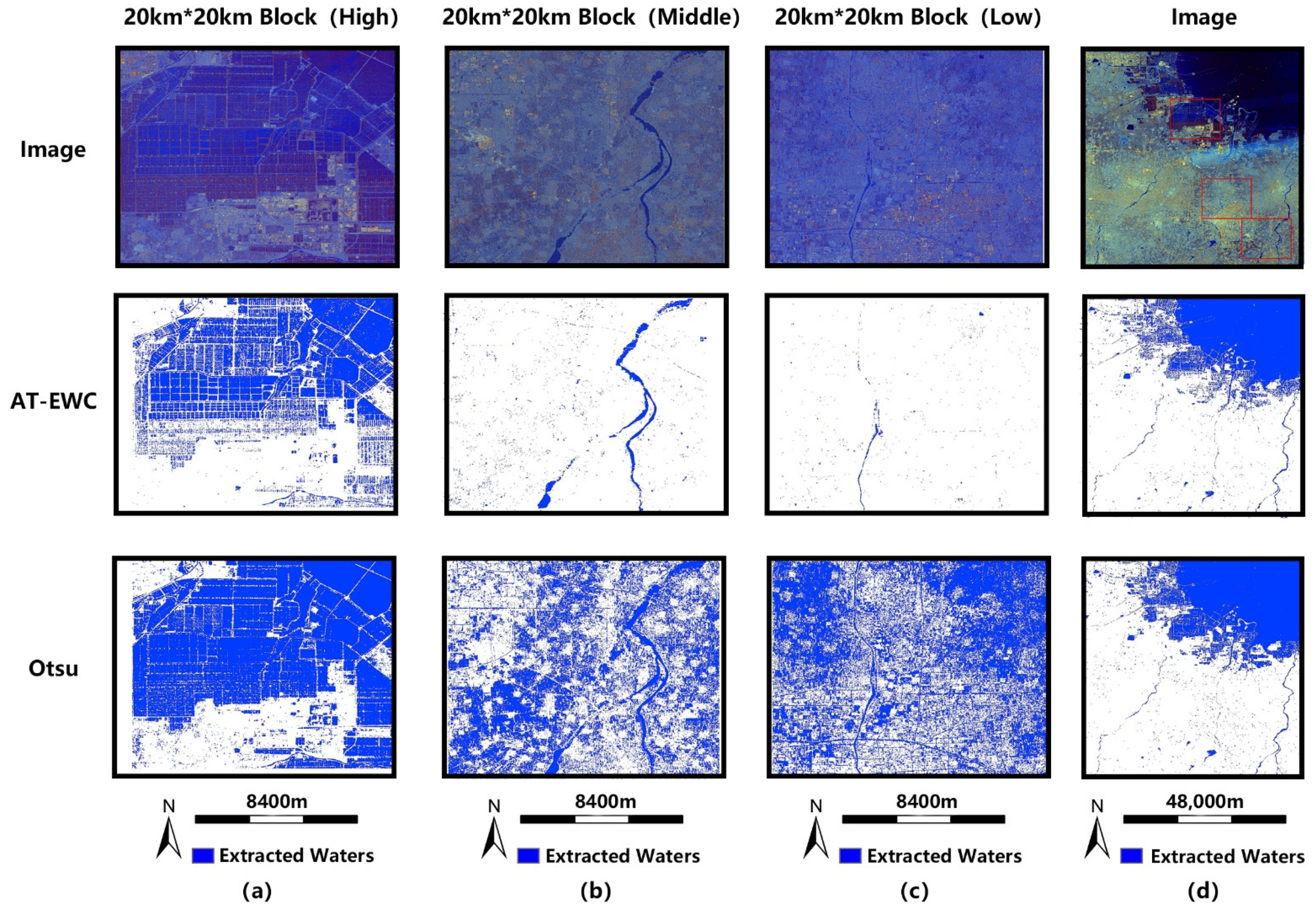
- The proposed method is tested over reservoir and watershed study sites in China. The area of water and non-water can be extracted quickly and accurately with our fully automated approach. The classification results of the two types of sites also show that our method is better than existing thresholding methods (e.g., Otsu [6]).
2. Study Area and Data
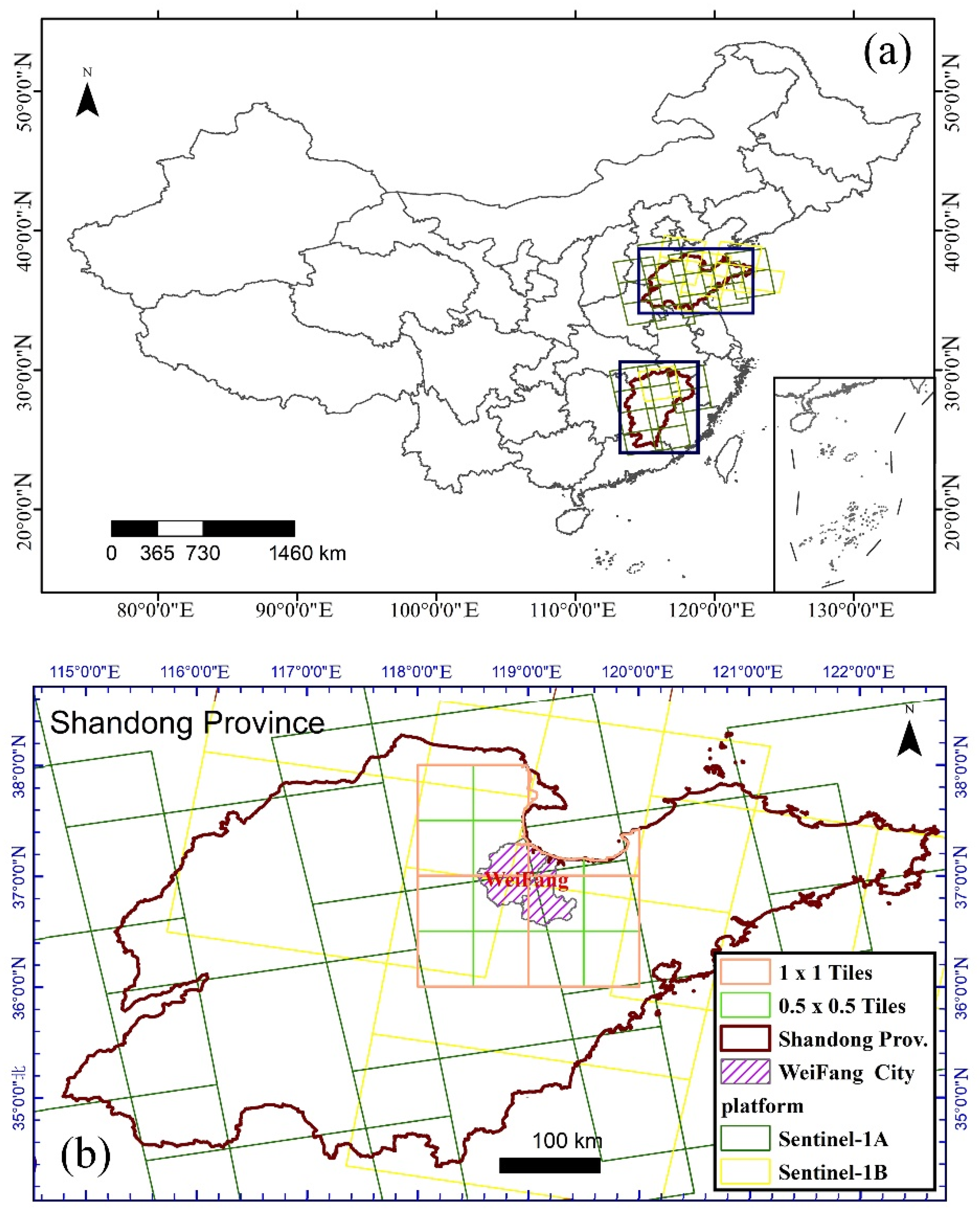
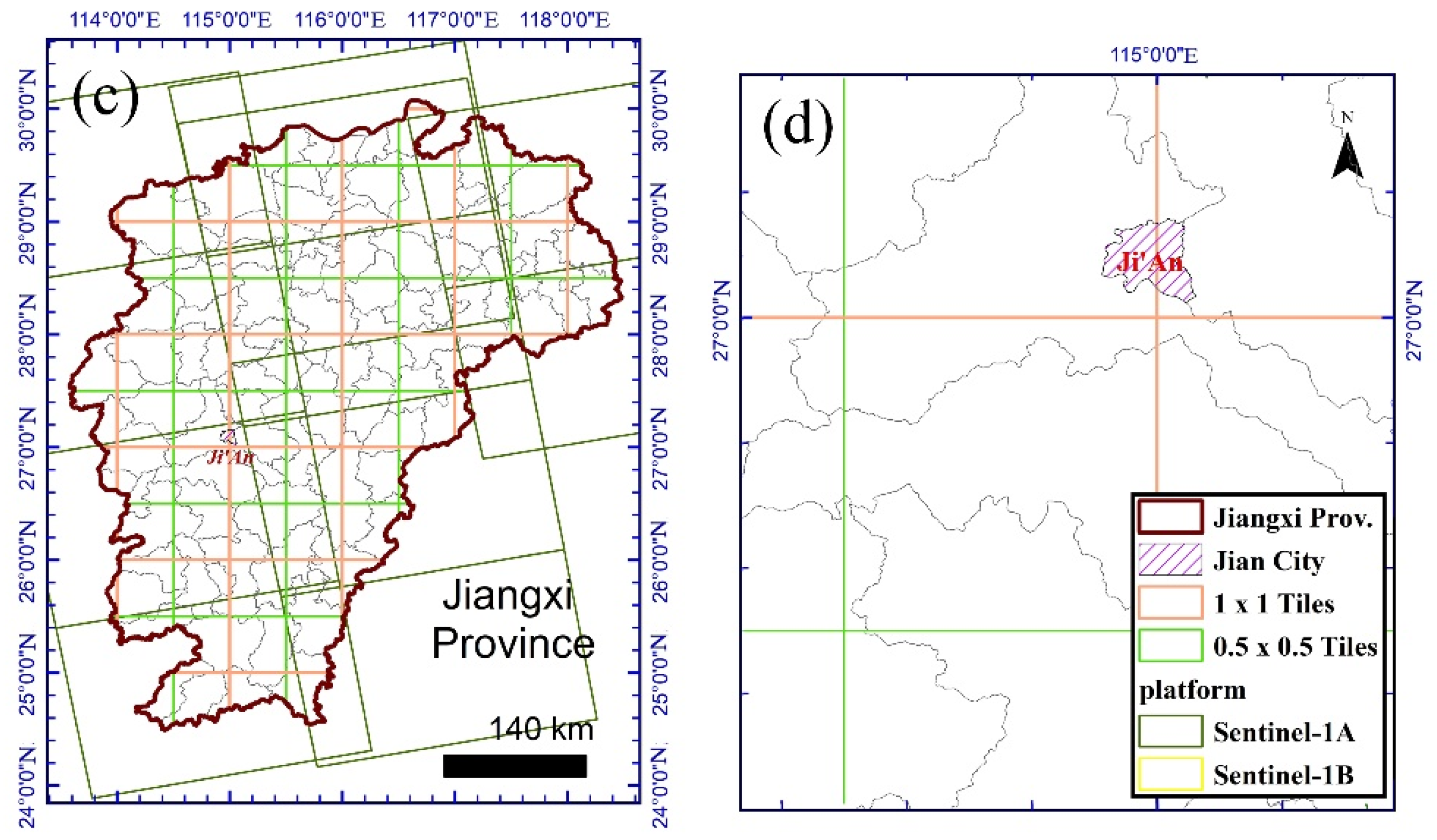
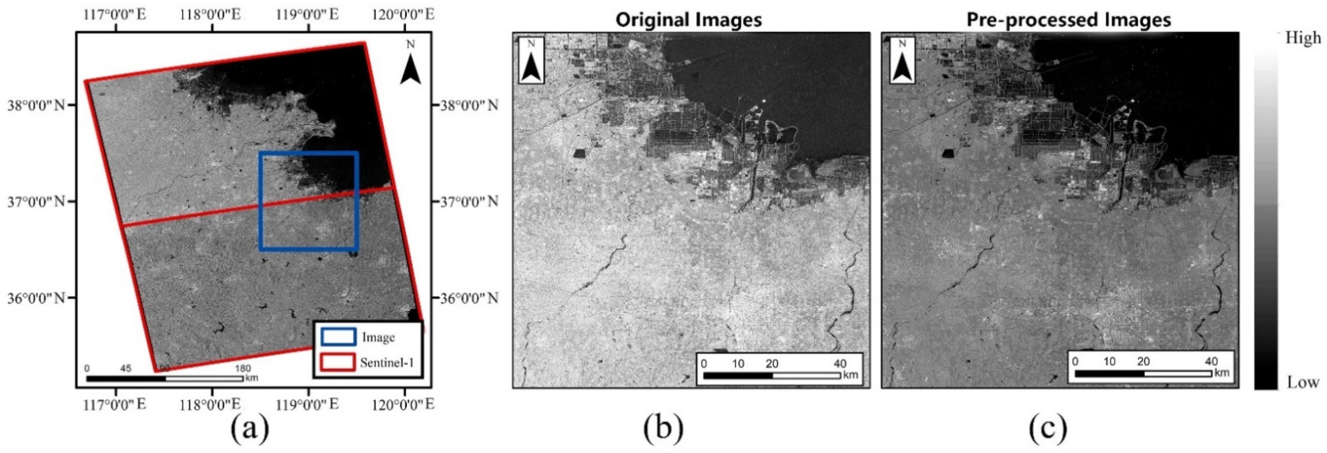
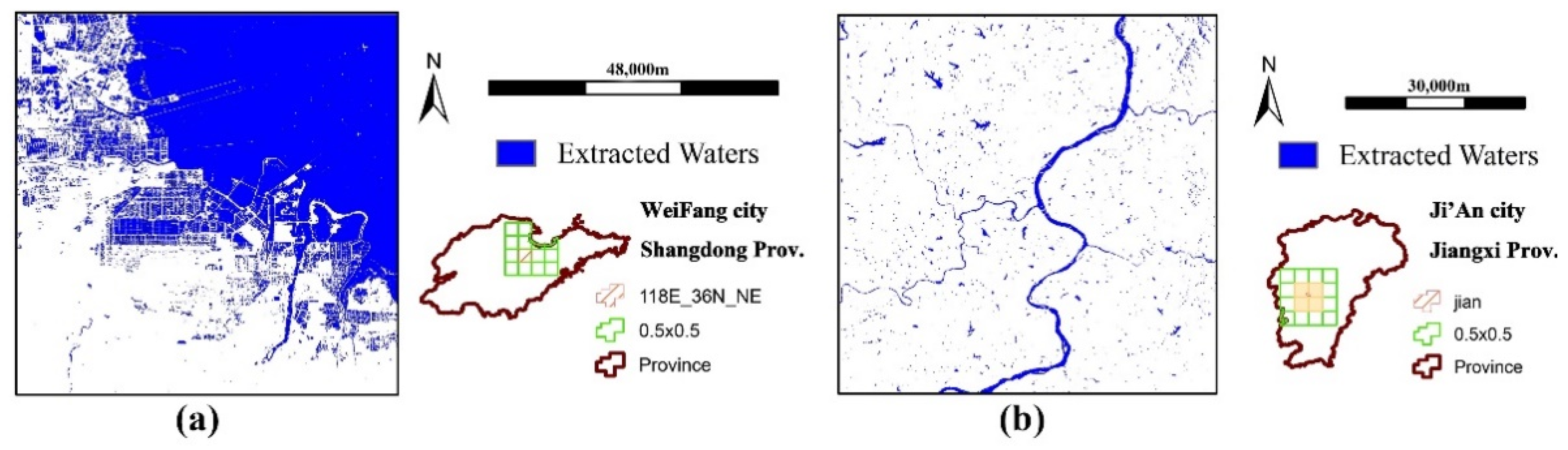
2.1. Study Area
2.2. Remote-Sensing Datasets
2.2.1. Sentinel-1 Data
2.2.2. Landsat Dataset on GEE
2.2.3. GF-3 Data
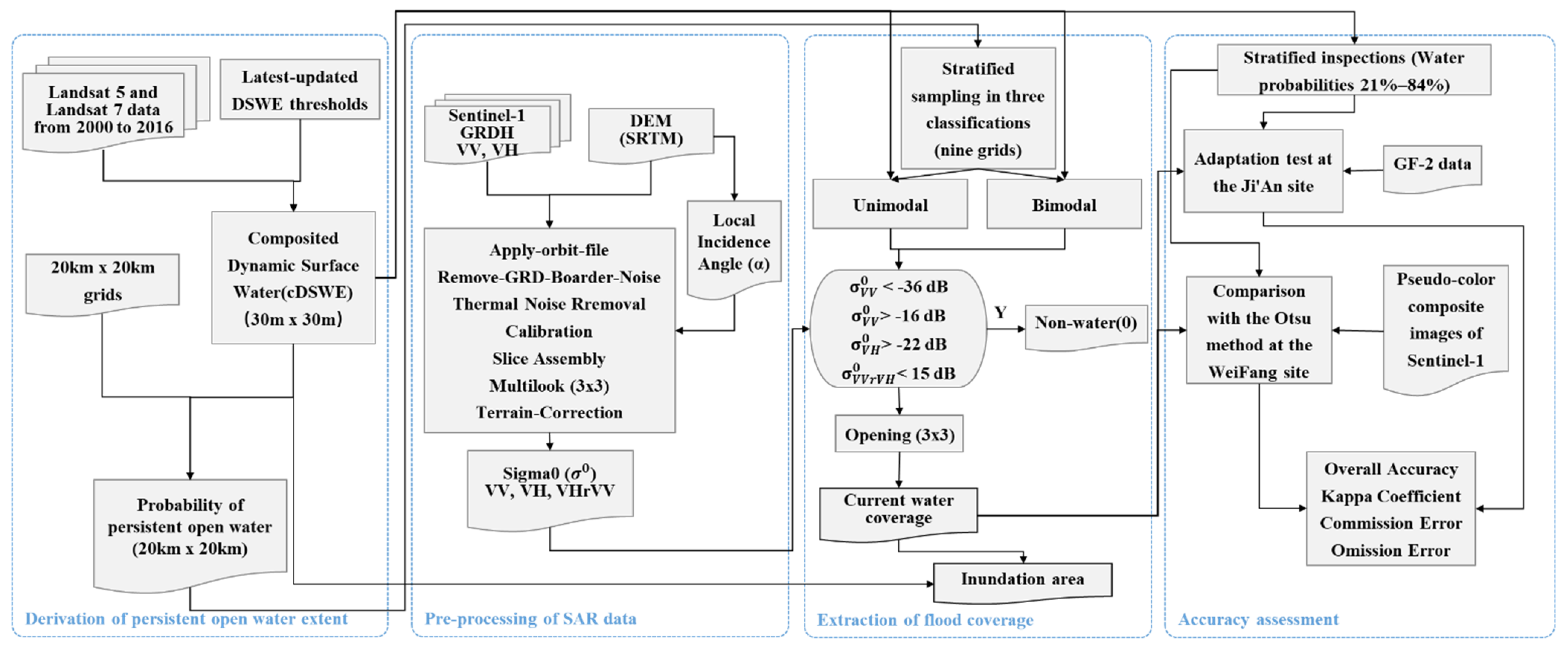
3. Methodology
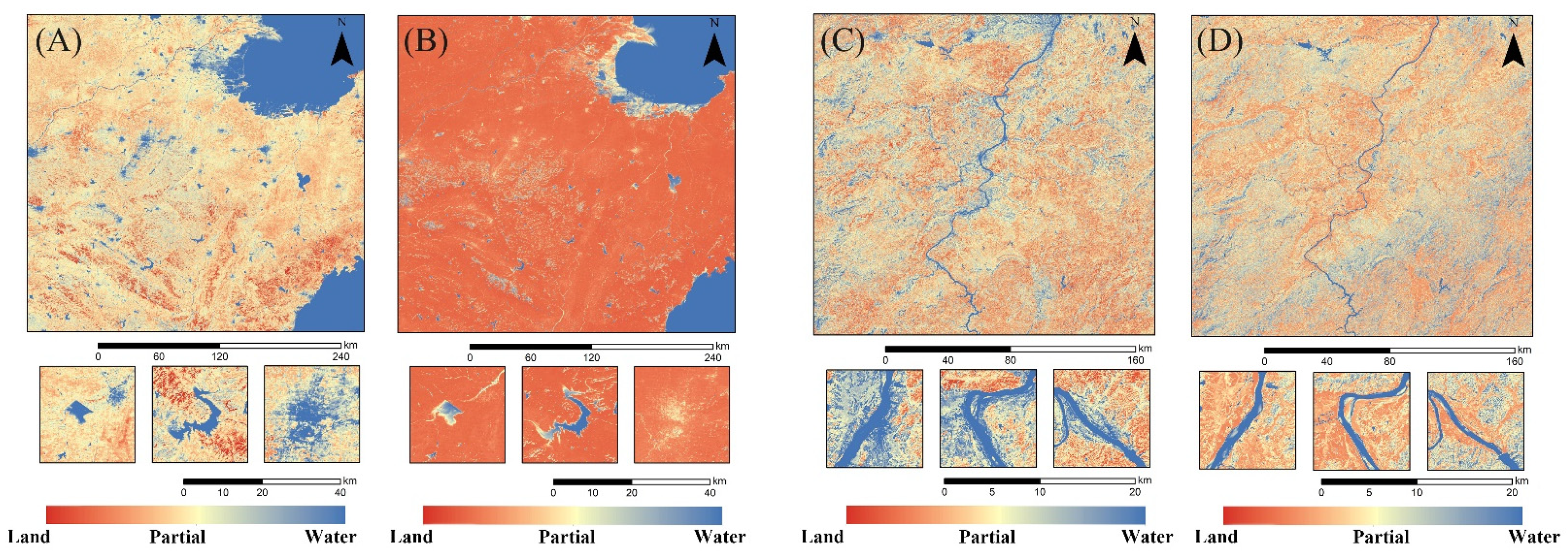
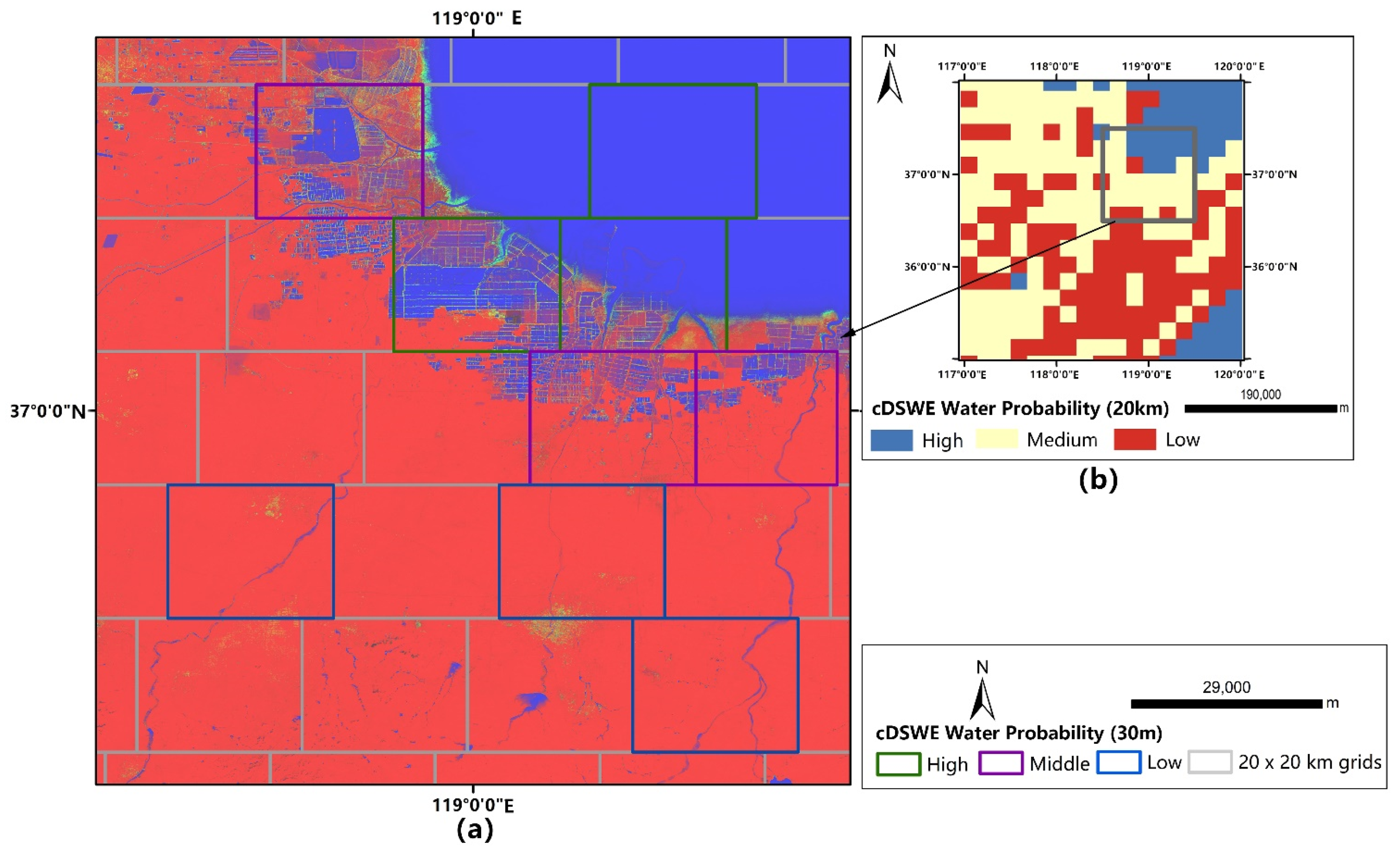
3.1. Derivation of Persistent Open-Water Extent from cDSWE
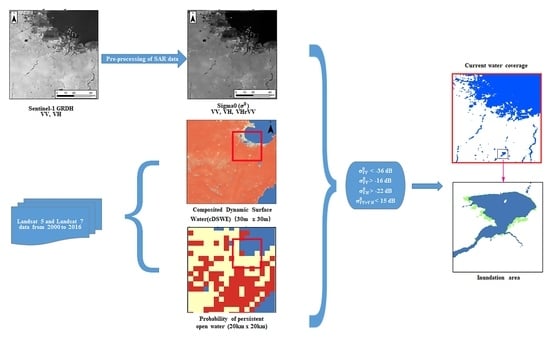
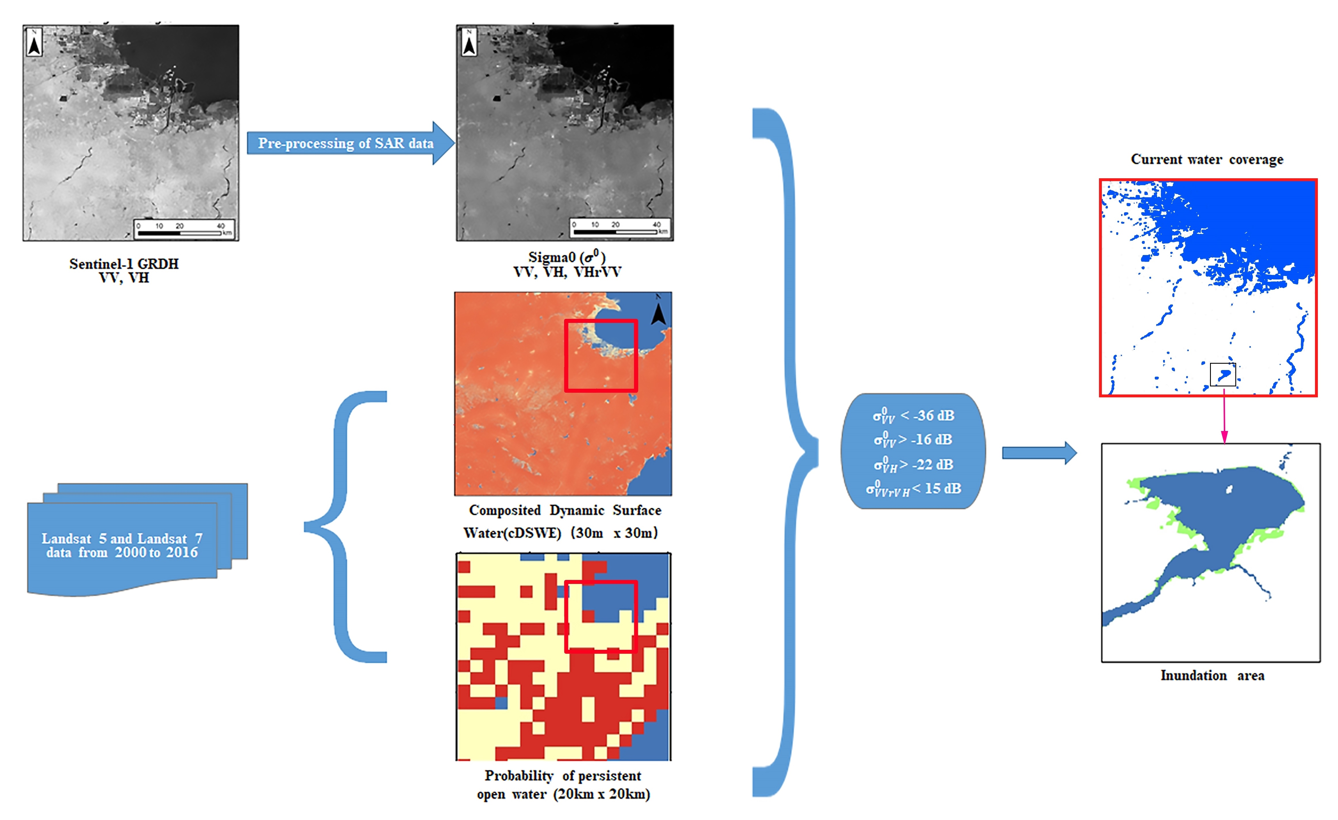
3.2. Pre-Processing of Sentinel-1 SAR Data
3.3. Extraction of Flood Coverage
3.4. Accuracy Assessment
4. Results
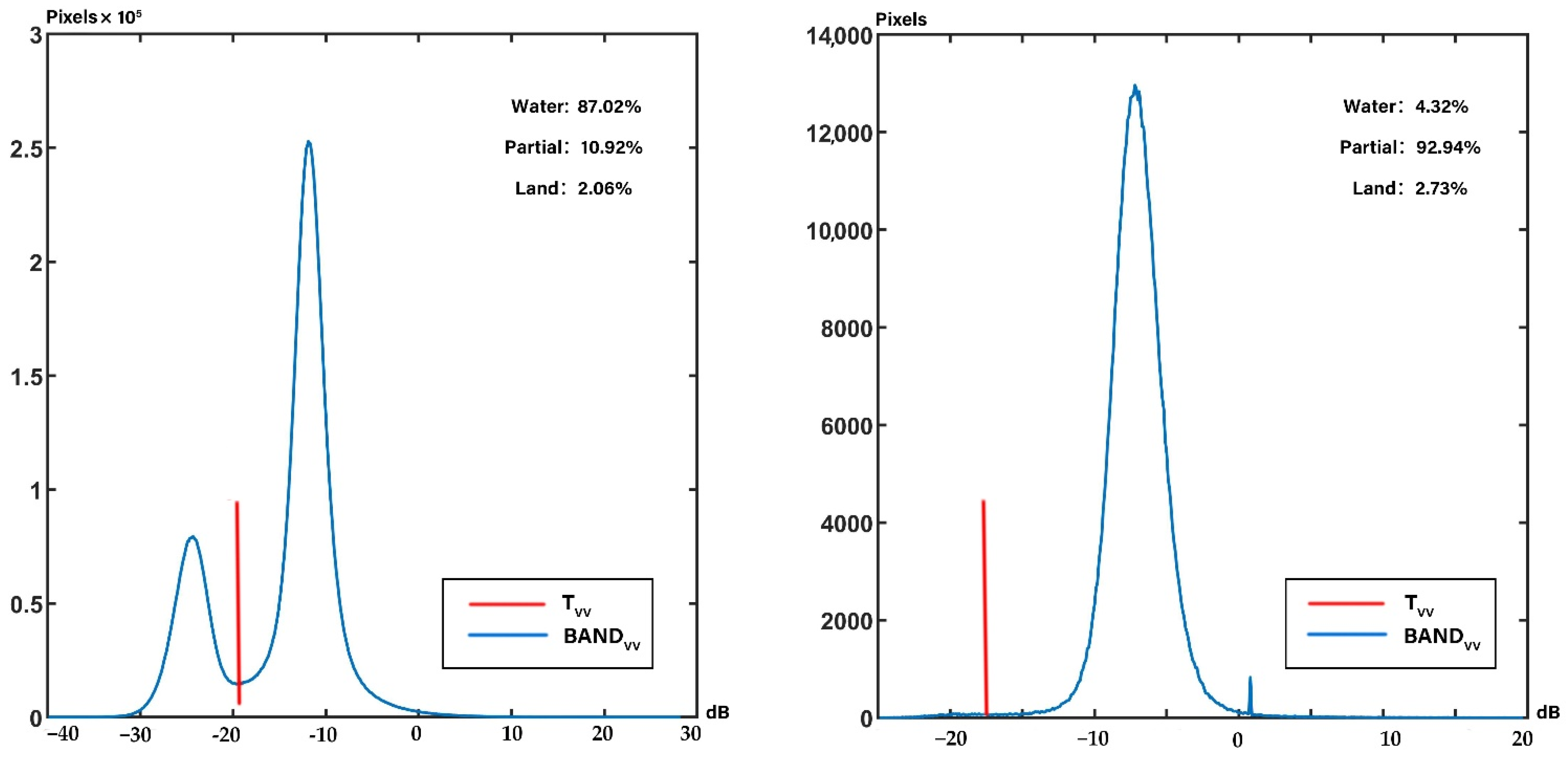
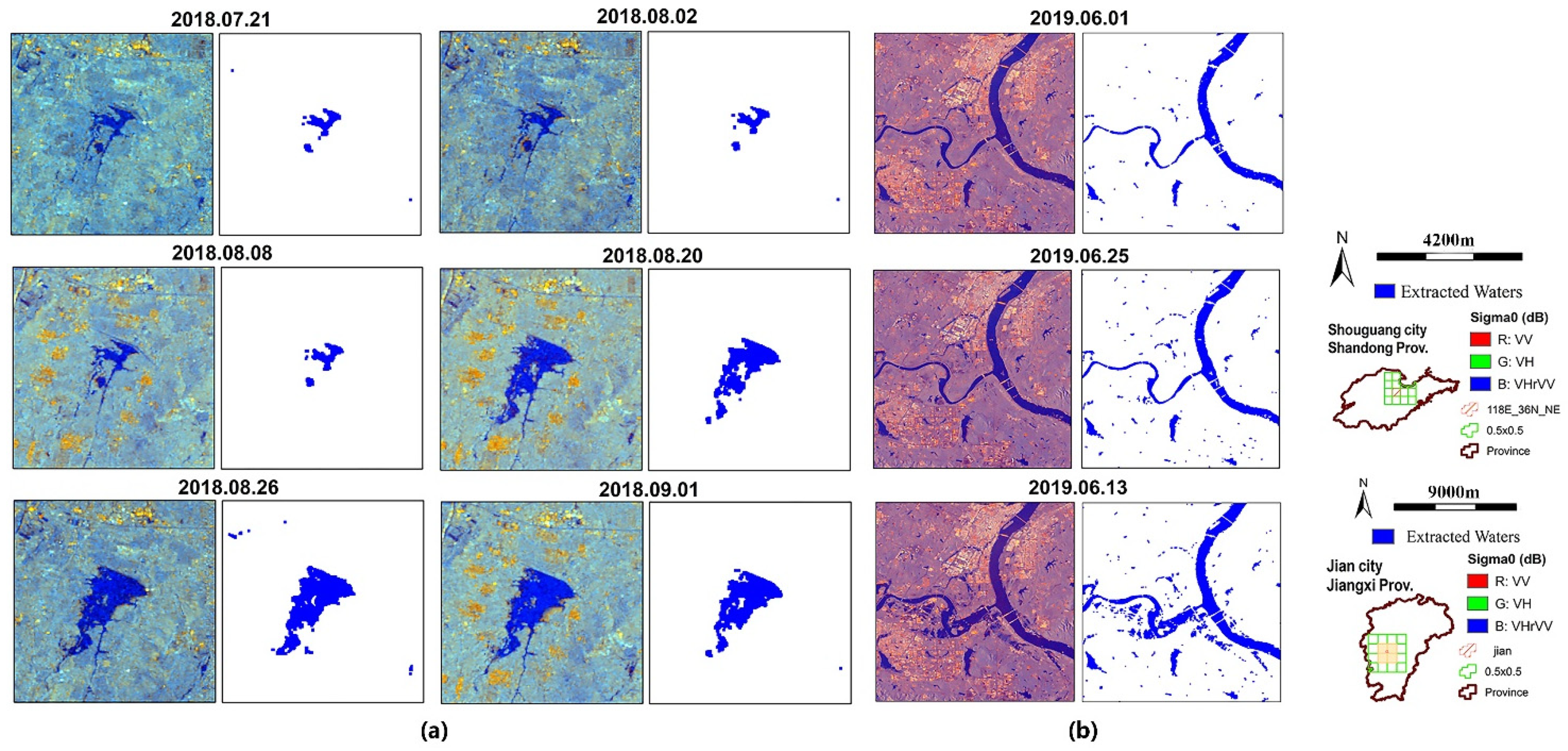
4.1. Time-Series Classification of Water and Non-Water
- —
- First, if > −16 dB, mark as water.
- —
- Second, if > −22 dB, mark as water.
- —
- Third, if < 15 dB, mark as water.
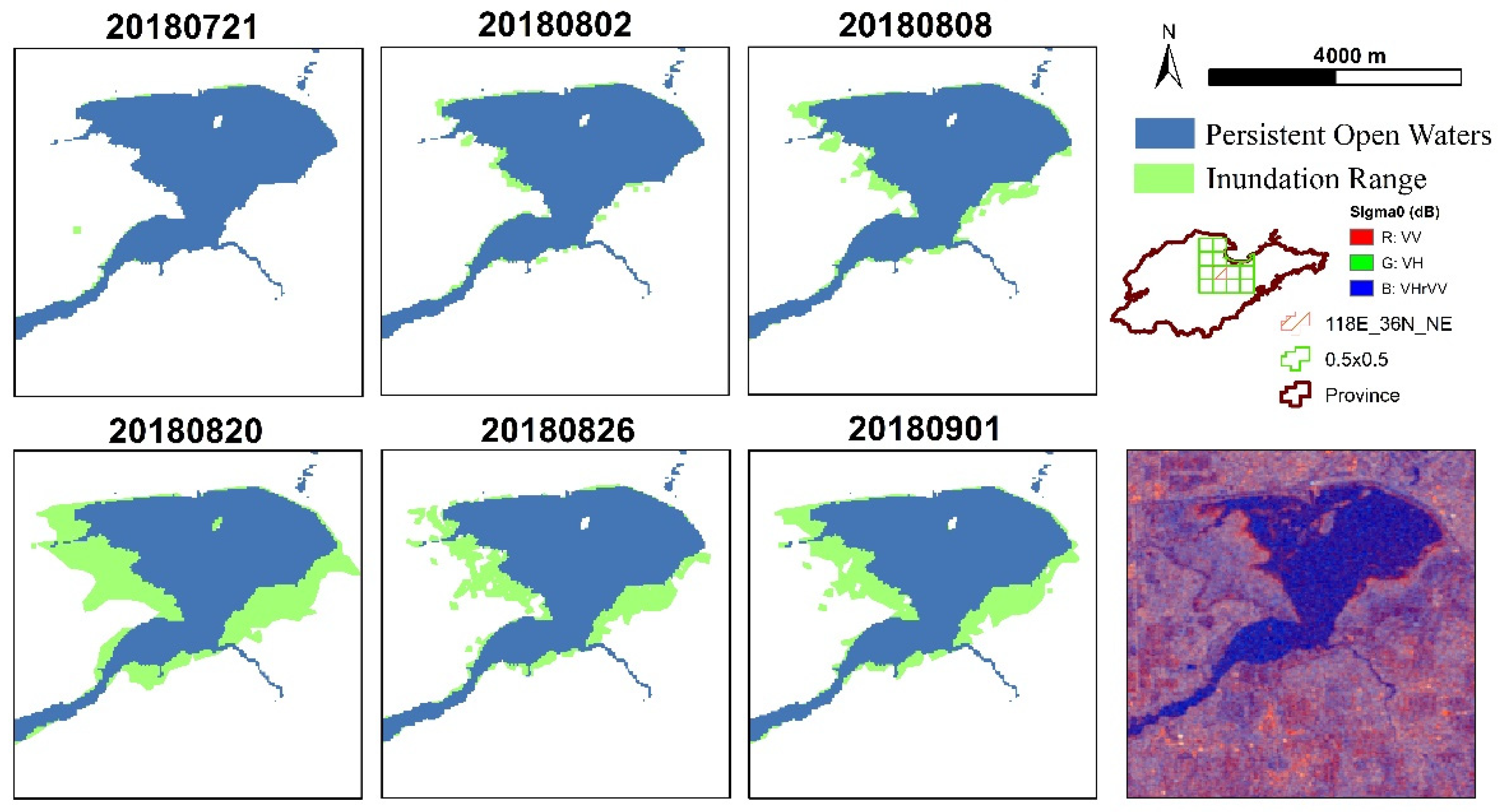
4.2. Inundation Range over Flood Event
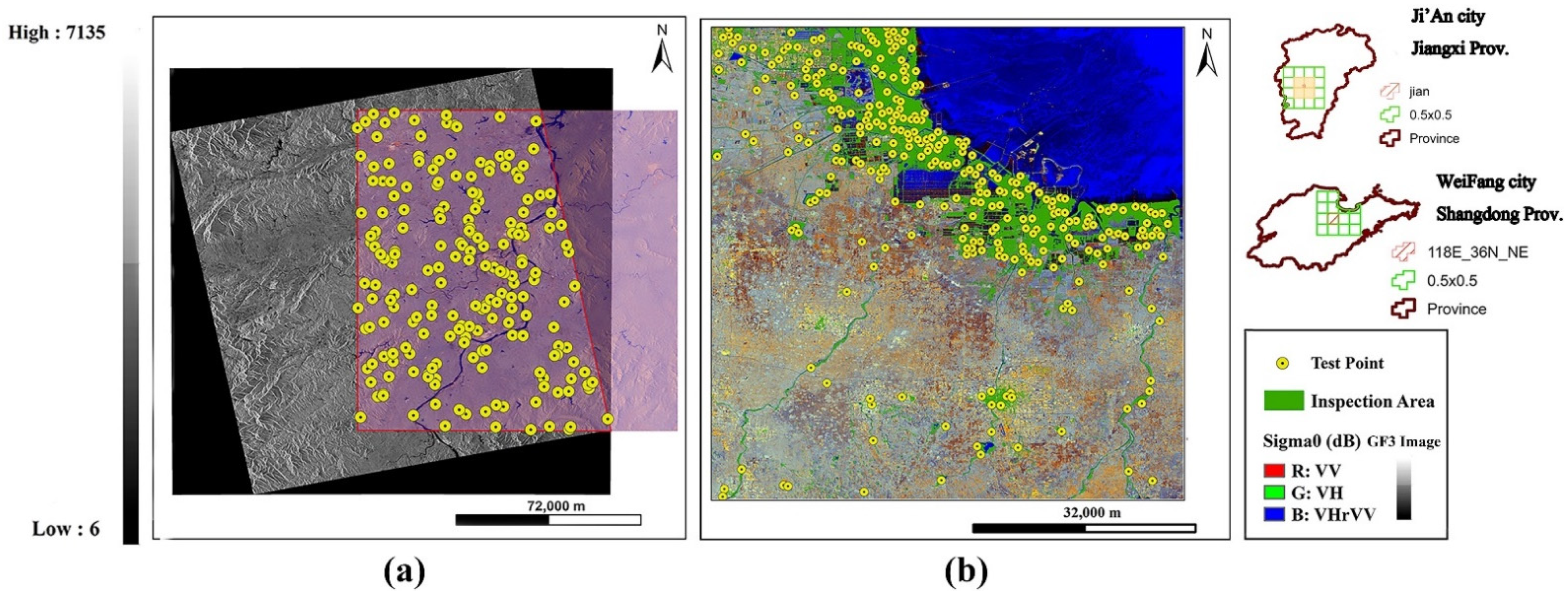
4.3. Accuracy Assessment at Two Sites
4.3.1. Adaptation of the Proposed Thresholds at the Ji’An Site
4.3.2. Comparison with the Otsu Method at the WeiFang Site
5. Discussion
5.1. Significance of This Study
5.2. Limitations and Potential Improvements
6. Conclusions
Author Contributions
Funding
Data Availability Statement
Acknowledgments
Conflicts of Interest
Appendix A
- --
- First, determine the latitude and longitude of the study area and the time of using the data; import the used data; set the name of the save folder.
- --
- Second, write a function that calculates the water body index (MNDWI, NDVI, MBSR, AWESH). The arguments of this function are calculated as follows:
- (a)
- Modified Normalized Difference Wetness Index (MNDWI) = (green − SWIR1)/(green + SWIR1)
- (b)
- Multi-band Spectral Relationship Visible (MBSRV) = green + red
- (c)
- Multi-band Spectral Relationship Near-Infrared (MBSRN) = NIR + SWIR1
- (d)
- Automated Water Extent Shadow (AWESH) = blue + (2.5 × green) − (1.5 × MBSRN) − (0.25 × SWIR2)
- (e)
- Normalized Difference Vegetation Index (NDVI) = (NIR − red)/(NIR + red)
- --
- Third, encode the five basic experimental functions of the DSWE algorithm.
- --
- Forth, in the code, write three classification functions corresponding to Water (Pixel Value = 1 and 2), Land (Pixel Value = 0) and Potential (Pixel Value = 3).
- --
- Fifth, output the final classification result to Google Drive.


References
- Goldberg, M. The Transition from Current Atmospheric Measurements to the NPOESS Era. In AGU Fall Meeting Abstracts; 2005; Available online: https://www.researchgate.net/publication/241370237_The_Transition_from_Current_Atmospheric_Measurements_to_the_NPOESS_Era (accessed on 25 October 2021).
- Voigt, S.; Giulio-Tonolo, F.; Lyons, J.; Kučera, J.; Jones, B.; Schneiderhan, T.; Platzeck, G.; Kaku, K.; Hazarika, M.K.; Czaran, L.; et al. Global trends in satellite-based emergency mapping. Science 2016, 353, 247–252. [Google Scholar] [CrossRef]
- Ritchie, J.C.; Schiebe, F.R.; Mchenry, J.R. Remote Sensing of Suspended Sediments in Surface Water. Photogramm. Eng. Remote Sens. 1976, 42, 1539–1545. [Google Scholar]
- Du, J.; Kimball, J.S.; Galantowicz, J.; Kim, S.B.; Chan, S.K.; Reichle, R.; Jones, L.A.; Watts, J.D. Assessing global surface water inundation dynamics using combined satellite information from SMAP, AMSR2 and Landsat. Remote Sens. Environ. 2018, 213, 1–17. [Google Scholar] [CrossRef]
- Wulder, M.A.; Masek, J.G.; Cohen, W.B.; Loveland, T.R.; Woodcock, C.E. Opening the archive: How free data has enabled the science and monitoring promise of Landsat. Remote Sens. Environ. 2012, 122, 2–10. [Google Scholar] [CrossRef]
- Otsu, N. A threshold selection method from gray-level histograms. IEEE Trans. Syst. Man Cybern. 1979, 9, 62–66. [Google Scholar] [CrossRef] [Green Version]
- Wu, H.; Liu, C.; Zhang, Y.; Sun, W. Water feature extraction from aerial-image fused with airborne LIDAR data. In Proceedings of the 2009 Joint Urban Remote Sensing Event, Shanghai, China, 20–22 May 2009. [Google Scholar]
- Feng, M.; Sexton, J.O.; Channan, S.; Townshend, J.R. A global, high-resolution (30-m) inland water body dataset for 2000: First results of a topographic–spectral classification algorithm. Int. J. Digit. Earth 2016, 9, 113–133. [Google Scholar] [CrossRef] [Green Version]
- Pickens, A.H.; Hansen, M.C.; Hancher, M.; Stehman, S.V.; Tyukavina, A.; Potapov, P.; Marroquin, B.; Sherani, Z. Mapping and sampling to characterize global inland water dynamics from 1999 to 2018 with full Landsat time-series. Remote Sens. Environ. 2020, 243, 111792. [Google Scholar] [CrossRef]
- Jones, J.W. Improved Automated Detection of Subpixel-Scale Inundation—Revised Dynamic Surface Water Extent (DSWE) Partial Surface Water Tests. Remote Sens. 2019, 11, 374. [Google Scholar] [CrossRef] [Green Version]
- Pekel, J.-F.; Cottam, A.; Gorelick, N.; Belward, A.S. High-resolution mapping of global surface water and its long-term changes. Nature 2016, 540, 418–422. [Google Scholar] [CrossRef]
- Yamazaki, D.; Trigg, M.A.; Ikeshima, D. Development of a global ~90m water body map using multi-temporal Landsat images. Remote Sens. Environ. 2015, 171, 337–351. [Google Scholar] [CrossRef]
- Tholey, N.; Clandillon, S.; Fraipont, P.D. The contribution of spaceborne SAR and optical data in monitoring flood events: Examples in northern and southern France. Hydrol. Process. 1997, 11, 1409–1413. [Google Scholar] [CrossRef]
- Solbo, S.; Pettinato, S.; Paloscia, S.; Santi, E.; Brusotti, P.; Solheim, I. Mapping of flooding in the Alessandria area with ERS. In Proceedings of the IGARSS 2004. 2004 IEEE International Geoscience and Remote Sensing Symposium, Anchorage, AK, USA, 20–24 September 2004. [Google Scholar]
- Bartsch, A.; Wagner, W.; Scipal, K.; Pathe, C.; Sabel, D.; Wolski, P. Global monitoring of wetlands—The value of ENVISAT ASAR Global mode. J. Environ. Manag. 2009, 90, 2226–2233. [Google Scholar] [CrossRef]
- Hess, L.; Melack, J.; Filoso, S.; Wang, Y. Delineation of inundated area and vegetation along the Amazon floodplain with the SIR-C synthetic aperture radar. IEEE Trans. Geosci. Remote Sens. 1995, 33, 896–904. [Google Scholar] [CrossRef] [Green Version]
- Henry, J.B.; Chastanet, P.; Fellah, K.; Desnos, Y.L. Envisat multi-polarized ASAR data for flood mapping. Int. J. Remote Sens. 2006, 27, 1921–1929. [Google Scholar] [CrossRef]
- Martinis, S.; Kersten, J.; Twele, A. A fully automated TerraSAR-X based flood service. ISPRS J. Photogramm. Remote Sens. 2015, 104, 203–212. [Google Scholar]
- Mason, D.C.; Speck, R.; Devereux, B.; Schumann, J.P.; Neal, J.C.; Bates, P.D. Flood Detection in Urban Areas Using TerraSAR-X. IEEE Trans. Geosci. Remote Sens. 2010, 48, 882–894. [Google Scholar] [CrossRef] [Green Version]
- Mason, D.C.; Davenport, I.J.; Neal, J.C.; Schumann, J.P.; Bates, P.D. Near Real-Time Flood Detection in Urban and Rural Areas Using High-Resolution Synthetic Aperture Radar Images. IEEE Trans. Geosci. Remote Sens. 2012, 50, 3041–3052. [Google Scholar] [CrossRef] [Green Version]
- Tanguy, M.; Chokmani, K.; Bernier, M.; Poulin, J.; Raymond, S. River flood mapping in urban areas combining Radarsat-2 data and flood return period data. Remote Sens. Environ. 2017, 198, 442–459. [Google Scholar] [CrossRef] [Green Version]
- Pulvirenti, L.; Chini, M.; Pierdicca, N.; Guerriero, L.; Ferrazzoli, P. Flood monitoring using multi-temporal COSMO-SkyMed data: Image segmentation and signature interpretation. Remote Sens. Environ. 2011, 115, 990–1002. [Google Scholar] [CrossRef]
- Twele, A.; Cao, W.; Plank, S.; Martinis, S. Sentinel-1-based flood mapping: A fully automated processing chain. Int. J. Remote Sens. 2016, 37, 2990–3004. [Google Scholar] [CrossRef]
- Laurila, P.; Modrzewski, R.; Cheng, T.; Campbell, B.; Yanni, V.G. Validation of ICEYE Small Satellite SAR Design for Ice Detection and Imaging. In Proceedings of the Arctic Technology Conference, St. John’s, NL, Canada, 24–26 October 2016. [Google Scholar]
- Huang, W.; DeVries, B.; Huang, C.; Lang, M.W.; Jones, J.W.; Creed, I.F.; Carroll, M.L. Automated Extraction of Surface Water Extent from Sentinel-1 Data. Remote Sens. 2018, 10, 797. [Google Scholar] [CrossRef] [Green Version]
- Bioresita, F.; Puissant, A.; Stumpf, A.; Malet, J.-P. A Method for Automatic and Rapid Mapping of Water Surfaces from Sentinel-1 Imagery. Remote Sens. 2018, 10, 217. [Google Scholar] [CrossRef] [Green Version]
- Liu, J.; Li, W.; Tian, Y. Automatic thresholding of gray-level pictures using two-dimension Otsu method. In Proceedings of the International Conference on Circuits and Systems, Shenzhen, China, 16–17 June 1991; Volume 1, pp. 325–327. [Google Scholar]
- Stutz, D.; Hermans, A.; Leibe, B. Superpixels: An evaluation of the state-of-the-art. Comput. Vis. Image Underst. 2018, 166, 1–27. [Google Scholar] [CrossRef] [Green Version]
- Lang, F.; Yang, J.; Yan, S.; Qin, F. Superpixel Segmentation of Polarimetric Synthetic Aperture Radar (SAR) Images Based on Generalized Mean Shift. Remote Sens. 2018, 10, 1592. [Google Scholar] [CrossRef] [Green Version]
- Ciecholewski, M. River channel segmentation in polarimetric SAR images: Watershed transform combined with average contrast maximisation. Expert Syst. Appl. 2017, 82, 196–215. [Google Scholar] [CrossRef]
- Cousty, J.; Bertrand, G.; Najman, L.; Couprie, M. Watershed Cuts: Thinnings, Shortest Path Forests, and Topological Watersheds. IEEE Trans. Pattern Anal. Mach. Intell. 2010, 32, 925–939. [Google Scholar] [CrossRef] [PubMed] [Green Version]
- Braga, A.M.; Marques, R.C.P.; Rodrigues, F.A.A.; Medeiros, F.N.S. A Median Regularized Level Set for Hierarchical Segmentation of SAR Images. IEEE Geosci. Remote Sens. Lett. 2017, 14, 1171–1175. [Google Scholar] [CrossRef]
- Jin, R.; Yin, J.; Zhou, W.; Yang, J. Level Set Segmentation Algorithm for High-Resolution Polarimetric SAR Images Based on a Heterogeneous Clutter Model. IEEE J. Sel. Top. Appl. Earth Obs. Remote Sens. 2017, 10, 4565–4579. [Google Scholar] [CrossRef]
- Kapur, J.N.; Sahoo, P.K.; Wong, A.K.C. A new method for gray-level picture thresholding using the entropy of the histogram. Comput. Vision, Graph. Image Process. 1985, 29, 273–285. [Google Scholar] [CrossRef]
- Pun, T. A new method for grey-level picture thresholding using the entropy of the histogram. Signal Process. 1980, 2, 223–237. [Google Scholar] [CrossRef]
- Sahoo, P.K.; Soltani, S.; Wong, A.K.C. A survey of thresholding techniques. Comput. Vis. Graph. Image Process. 1988, 41, 233–260. [Google Scholar] [CrossRef]
- Sekertekin, A. A Survey on Global Thresholding Methods for Mapping Open Water Body Using Sentinel-2 Satellite Imagery and Normalized Difference Water Index. Arch. Comput. Methods Eng. 2021, 28, 1335–1347. [Google Scholar] [CrossRef]
- Wang, Z.; Zhang, R.; Zhang, Q.; Zhu, Y.; Huang, B.; Lu, Z. An Automatic Thresholding Method For Water Body Detection From SAR Image. In Proceedings of the 2019 IEEE International Conference on Signal, Information and Data Processing (ICSIDP), Chongqing, China, 11–13 December 2019; pp. 1–4. [Google Scholar]
- Liang, J.; Liu, D. A local thresholding approach to flood water delineation using Sentinel-1 SAR imagery. ISPRS J. Photogramm. Remote Sens. 2020, 159, 53–62. [Google Scholar] [CrossRef]
- Hong, Z.; Fan, J. A Threshold Segmentation Method for Sparse Histogram Image. In Proceedings of the 2009 Sixth International Conference on Fuzzy Systems and Knowledge Discovery, Tianjin, China, 14–16 August 2009; pp. 340–344. [Google Scholar]
- Coudray, N.; Buessler, J.L.; Urban, J.P. Robust threshold estimation for images with unimodal histograms. Pattern Recognit. Lett. 2010, 31, 1010–1019. [Google Scholar] [CrossRef] [Green Version]
- Maniar, H.; Ryali, S.; Kulkarni, M.S.; Abubakar, A. 2018 Machine-learning methods in geoscience. In SEG Technical Program Expanded Abstracts; Society of Exploration Geophysicists: Tulsa, OK, USA, 2018; pp. 4638–4642. [Google Scholar]
- Shahabi, H.; Shirzadi, A.; Ghaderi, K.; Omidvar, E.; Al-Ansari, N.; Clague, J.J.; Geertsema, M.; Khosravi, K.; Amini, A.; Bahrami, S.; et al. Flood Detection and Susceptibility Mapping Using Sentinel-1 Remote Sensing Data and a Machine Learning Approach: Hybrid Intelligence of Bagging Ensemble Based on K-Nearest Neighbor Classifier. Remote Sens. 2020, 12, 266. [Google Scholar] [CrossRef] [Green Version]
- Lv, W.; Yu, Q.; Yu, W. Water extraction in SAR images using GLCM and Support Vector Machine. In IEEE 10th International Conference on Signal Processing Proceedings; IEEE: Piscataway, NJ, USA, 2010; pp. 740–743. [Google Scholar]
- Acharya, T.D.; Subedi, A.; Dong, H.L. Evaluation of Machine Learning Algorithms for Surface Water Extraction in a Landsat 8 Scene of Nepal. Sensors 2019, 19, 2769. [Google Scholar] [CrossRef] [Green Version]
- Chen, Y.; Fan, R.; Yang, X.; Wang, J.; Latif, A. Extraction of Urban Water Bodies from High-Resolution Remote-Sensing Imagery Using Deep Learning. Water 2018, 10, 585. [Google Scholar] [CrossRef] [Green Version]
- Tyralis, H.; Papacharalampous, G.; Langousis, A. A Brief Review of Random Forests for Water Scientists and Practitioners and Their Recent History in Water Resources. Water 2019, 11, 910. [Google Scholar] [CrossRef] [Green Version]
- An, C.; Niu, Z.; Li, Z.; Chen, Z. Otsu Threshold Comparison and SAR Water Segmentation Result. J. Electron. Inf. Technol. 2010, 32, 2215–2219. [Google Scholar] [CrossRef]
- Liu, D.; Yu, J. Otsu Method and K-means. In Proceedings of the 2009 Ninth International Conference on Hybrid Intelligent Systems, Shenyang, China, 12–14 August 2009; Volume 1, pp. 344–349. [Google Scholar]
- Jia, H.; Sun, K.; Song, W.; Peng, X.; Lang, C.; Li, Y. Multi-Strategy Emperor Penguin Optimizer for RGB Histogram-Based Color Satellite Image Segmentation Using Masi Entropy. IEEE Access 2019, 7, 134448–134474. [Google Scholar] [CrossRef]
- Nakmuenwai, P.; Yamazaki, F.; Liu, W. Automated Extraction of Inundated Areas from Multi-Temporal Dual-Polarization RADARSAT-2 Images of the 2011 Central Thailand Flood. Remote Sens. 2017, 9, 78. [Google Scholar] [CrossRef] [Green Version]
- Chini, M.; Hostache, R.; Giustarini, L.; Matgen, P. A Hierarchical Split-Based Approach for Parametric Thresholding of SAR Images: Flood Inundation as a Test Case. IEEE Trans. Geosci. Remote Sens. 2017, 55, 6975–6988. [Google Scholar] [CrossRef]
- Xiong, J.; Thenkabail, P.S.; Tilton, J.C.; Gumma, M.K.; Teluguntla, P.; Oliphant, A.; Congalton, R.G.; Yadav, K.; Gorelick, N. Nominal 30-m Cropland Extent Map of Continental Africa by Integrating Pixel-Based and Object-Based Algorithms Using Sentinel-2 and Landsat-8 Data on Google Earth Engine. Remote Sens. 2017, 9, 1065. [Google Scholar] [CrossRef] [Green Version]
- Imandoust, S.B.; Bolandraftar, M. Application of K-nearest neighbor (KNN) approach for predicting economic events theoretical background. Int. J. Eng. Res. Appl. 2013, 3, 605–610. [Google Scholar]
- Mahdianpari, M.; Salehi, B.; Mohammadimanesh, F.; Homayouni, S.; Gill, E. The First Wetland Inventory Map of Newfoundland at a Spatial Resolution of 10 m Using Sentinel-1 and Sentinel-2 Data on the Google Earth Engine Cloud Computing Platform. Remote Sens. 2018, 11, 43. [Google Scholar] [CrossRef] [Green Version]
- Johansen, K.; Phinn, S.; Taylor, M. Mapping woody vegetation clearing in Queensland, Australia from Landsat imagery using the Google Earth Engine. Remote Sens. Appl. Soc. Environ. 2015, 1, 36–49. [Google Scholar] [CrossRef]
- Tsai, Y.H.; Stow, D.; Chen, H.L.; Lewison, R.; An, L.; Shi, L. Mapping Vegetation and Land Use Types in Fanjingshan National Nature Reserve Using Google Earth Engine. Remote Sens. 2018, 10, 927. [Google Scholar] [CrossRef] [Green Version]
- Torres, R.; Snoeij, P.; Geudtner, D.; Bibby, D.; Davidson, M.; Attema, E.; Potin, P.; Rommen, B.; Floury, N.; Brown, M.; et al. GMES Sentinel-1 mission. Remote Sens. Environ. 2012, 120, 9–24. [Google Scholar] [CrossRef]
- Simmons, A.; Fellous, J.L.; Ramaswamy, V.; Trenberth, K.; Asrar, G.; Balmaseda, M.; Burrows, J.P.; Ciais, P.; Drinkwater, M.; Friedlingstein, P.; et al. Observation and integrated Earth-system science: A roadmap for 2016–2025. Adv. Space Res. 2016, 57, 2037–2103. [Google Scholar] [CrossRef] [Green Version]
- Williams, D.L.; Goward, S.; Arvidson, T. Landsat: Yesterday, Today, and Tomorrow. Photogramm. Eng. Remote Sens. 2006, 72, 1171–1178. [Google Scholar] [CrossRef]
- Gorelick, N.; Hancher, M.; Dixon, M.; Ilyushchenko, S.; Thau, D.; Moore, R. Google Earth Engine: Planetary-scale geospatial analysis for everyone. Remote Sens. Environ. 2017, 202, 18–27. [Google Scholar] [CrossRef]
- Goldblatt, R.; Rivera Ballesteros, A.; Burney, J. High Spatial Resolution Visual Band Imagery Outperforms Medium Resolution Spectral Imagery for Ecosystem Assessment in the Semi-Arid Brazilian Sertão. Remote Sens. 2017, 9, 1336. [Google Scholar] [CrossRef] [Green Version]
- Robinson, N.P.; Allred, B.W.; Jones, M.O.; Moreno, A.; Kimball, J.S.; Naugle, D.E.; Erickson, T.A.; Richardson, A.D. A Dynamic Landsat Derived Normalized Difference Vegetation Index (NDVI) Product for the Conterminous United States. Remote Sens. 2017, 9, 863. [Google Scholar] [CrossRef] [Green Version]
- Hansen, M.C.; Potapov, P.V.; Moore, R.; Hancher, M.; Turubanova, S.A.; Tyukavina, A.; Thau, D.; Stehman, S.V.; Goetz, S.J.; Loveland, T.R.; et al. High-Resolution Global Maps of 21st-Century Forest Cover Change. Science 2013, 342, 850–853. [Google Scholar] [CrossRef] [PubMed] [Green Version]
- He, M.; Kimball, J.S.; Maneta, M.P.; Maxwell, B.D.; Moreno, A.; Beguería, S.; Wu, X. Regional Crop Gross Primary Productivity and Yield Estimation Using Fused Landsat-MODIS Data. Remote Sens. 2018, 10, 372. [Google Scholar] [CrossRef] [Green Version]
- Aguilar, R.; Zurita-Milla, R.; Izquierdo-Verdiguier, E.; De By, R.A. A Cloud-Based Multi-Temporal Ensemble Classifier to Map Smallholder Farming Systems. Remote Sens. 2018, 10, 729. [Google Scholar] [CrossRef] [Green Version]
- Qiu, X.; Ding, C.; Lei, B.; Han, B.; Li, F. A Novel Proposal of Gaofen-3 Satellite Constellation for Multi-Applications. ISPRS-Int. Arch. Photogramm. Remote Sens. Spat. Inf. Sci. 2017, XLII-2/W7, 635–639. [Google Scholar] [CrossRef] [Green Version]


| Method | Category | Pros and Cons | Example |
|---|---|---|---|
| Image Thresholding | Otsu Binarization | an exhaustive algorithm for searching the global optimal threshold; easy to be severely corrupted by noise | [6,27,48,49] |
| Entropy Threshold | features are easy to select and replace; a large amount of computation | [34,35,40,50] | |
| Bimodal Histogram | effectiveness and efficiency; strict requirements are necessary for the shape of the histogram; low applicability | [50,51,52] | |
| Machine Learning | Support Vector Machine (SVM) | achieves accurate extraction results and improves the influence of noise; the parameters greatly affect the classification results | [44,45,53] |
| K-Nearest Neighbor (KNN) | decrease the overfitting and variance problems in the training dataset; a large amount of calculation and debugging is required | [43,54] | |
| Random Forest (RF) | the most accurate method for the classification of water bodies at present; a training dataset is difficult to obtain, and the classifier training is relatively time-consuming | [45,47,55,56,57] |
| Data | Overall Accuracy | Kappa Coefficient | Commission Error | Omission Error | ||
|---|---|---|---|---|---|---|
| Land | Water | Land | Water | |||
| 1 June 2019 | 95.00% | 0.7715 | 3.41% | 16.67% | 2.30% | 23.08% |
| 13 June 2019 | 96.00% | 0.8172 | 2.84% | 12.50% | 1.72% | 19.23% |
| 25 June 2019 | 94.50% | 0.7443 | 3.95% | 17.39% | 2.30% | 26.92% |
| Data | Overall Accuracy | Kappa Coefficient | Commission Error | Omission Error | ||
|---|---|---|---|---|---|---|
| Land | Water | Land | Water | |||
| 1 June 2019 | 95.00% | 0.7790 | 2.87% | 19.23% | 2.87% | 19.23% |
| 13 June 2019 | 96.50% | 0.8427 | 2.29% | 12.00% | 1.72% | 15.38% |
| 25 June 2019 | 95.50% | 0.7978 | 2.86% | 16.00% | 2.30% | 19.23% |
| Type | Threshold | Overall Accuracy | Kappa Coefficient | Commission Error | Omission Error | ||
|---|---|---|---|---|---|---|---|
| Land | Water | Land | Water | ||||
| Image | AT-EWC | 95.50% | 0.9080 | 3.57% | 2.65% | 3.57% | 2.65% |
| Otsu | 94.50% | 0.8876 | 4.39% | 6.98% | 5.22% | 5.88% | |
| (−) | (0.01) | (0.02) | (−0.01) | (−0.04) | (−0.02) | (−0.03) | |
| 20 km × 20 km Block (High) | AT-EWC | 96.00% | 0.9199 | 2.91% | 5.15% | 4.76% | 3.16% |
| Otsu | 95.00% | 0.8997 | 4.76% | 5.26% | 4.76% | 5.26% | |
| (−) | (0.01) | (0.02) | (−0.02) | (0.00) | (0.00) | (−0.02) | |
| 20 km × 20 km Block (Middle) | AT-EWC | 96.00% | 0.8947 | 2.03% | 9.62% | 3.33% | 6.00% |
| Otsu | 84.00% | 0.6364 | 2.42% | 38.16% | 19.33% | 6.00% | |
| (−) | (0.12) | (0.26) | (0.00) | (−0.29) | (−0.16) | (0.00) | |
| 20 km × 20 km Block (Low) | AT-EWC | 97.50% | 0.8697 | 1.12% | 13.64% | 1.68% | 9.52% |
| Otsu | 81.00% | 0.4136 | 0.69% | 66.07% | 20.56% | 5.00% | |
| (−) | (0.17) | (0.46) | (0.00) | (−0.52) | (−0.19) | (0.05) | |
| Time(s) | #1 * | #2 | #3 | #4 | #5 | #6 | #7 | #8 | #9 | Average |
|---|---|---|---|---|---|---|---|---|---|---|
| AT-EWC | 0.09 | 0.09 | 0.11 | 0.09 | 0.09 | 0.09 | 0.09 | 0.09 | 0.19 | 0.10 |
| Otsu | 0.29 | 0.26 | 0.24 | 0.23 | 0.23 | 0.23 | 0.25 | 0.29 | 0.24 | 0.25 |
Publisher’s Note: MDPI stays neutral with regard to jurisdictional claims in published maps and institutional affiliations. |
© 2021 by the authors. Licensee MDPI, Basel, Switzerland. This article is an open access article distributed under the terms and conditions of the Creative Commons Attribution (CC BY) license (https://creativecommons.org/licenses/by/4.0/).
Share and Cite
Chen, S.; Huang, W.; Chen, Y.; Feng, M. An Adaptive Thresholding Approach toward Rapid Flood Coverage Extraction from Sentinel-1 SAR Imagery. Remote Sens. 2021, 13, 4899. https://doi.org/10.3390/rs13234899
Chen S, Huang W, Chen Y, Feng M. An Adaptive Thresholding Approach toward Rapid Flood Coverage Extraction from Sentinel-1 SAR Imagery. Remote Sensing. 2021; 13(23):4899. https://doi.org/10.3390/rs13234899
Chicago/Turabian StyleChen, Shujie, Wenli Huang, Yumin Chen, and Mei Feng. 2021. "An Adaptive Thresholding Approach toward Rapid Flood Coverage Extraction from Sentinel-1 SAR Imagery" Remote Sensing 13, no. 23: 4899. https://doi.org/10.3390/rs13234899