
Continuous Change Mapping to Understand Wetland Quantity and Quality Evolution and Driving Forces: A Case Study in the Liao River Estuary from 1986 to 2018

Abstract
:1. Introduction
2. Data and Methods
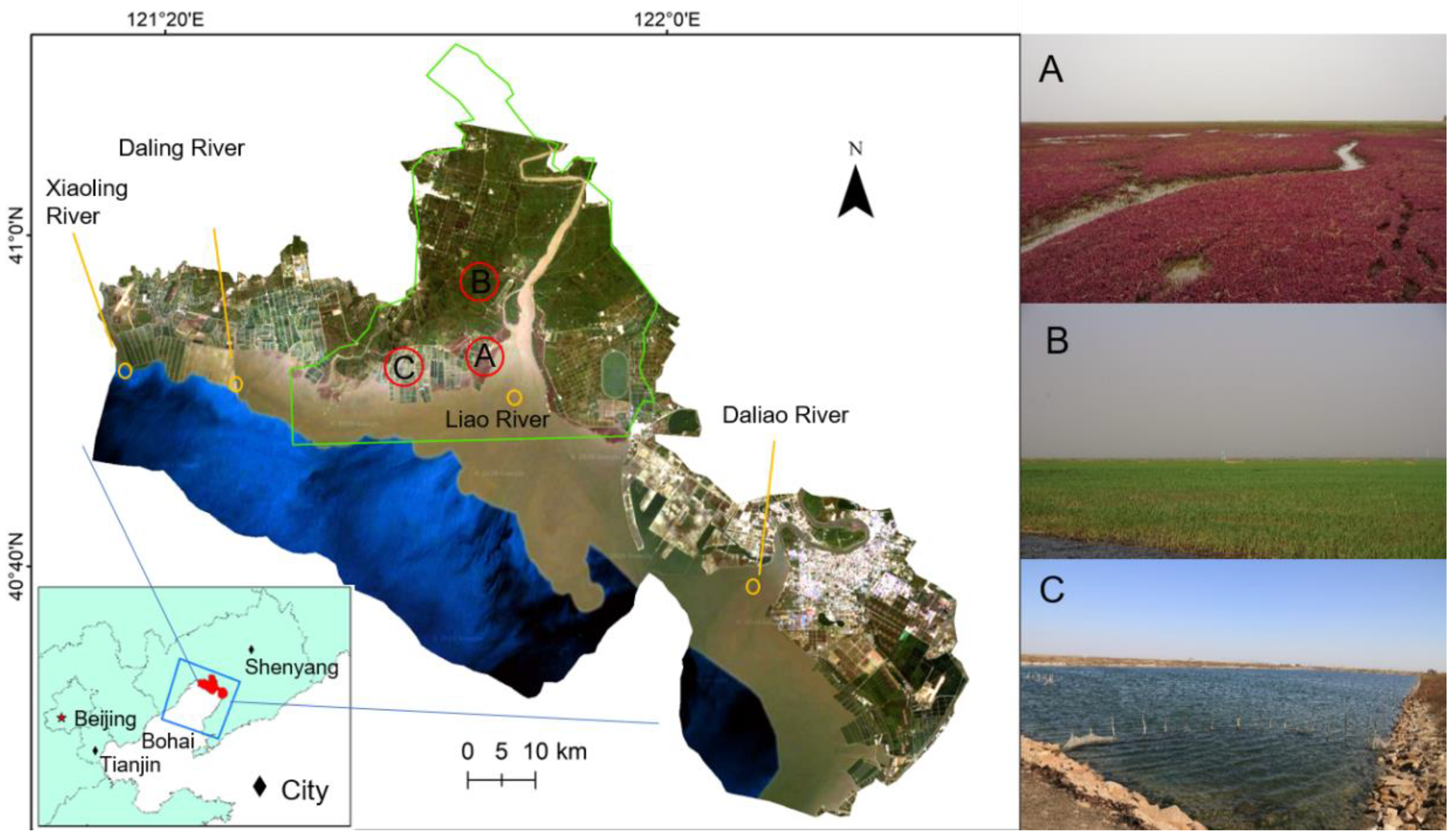
2.1. Study Area
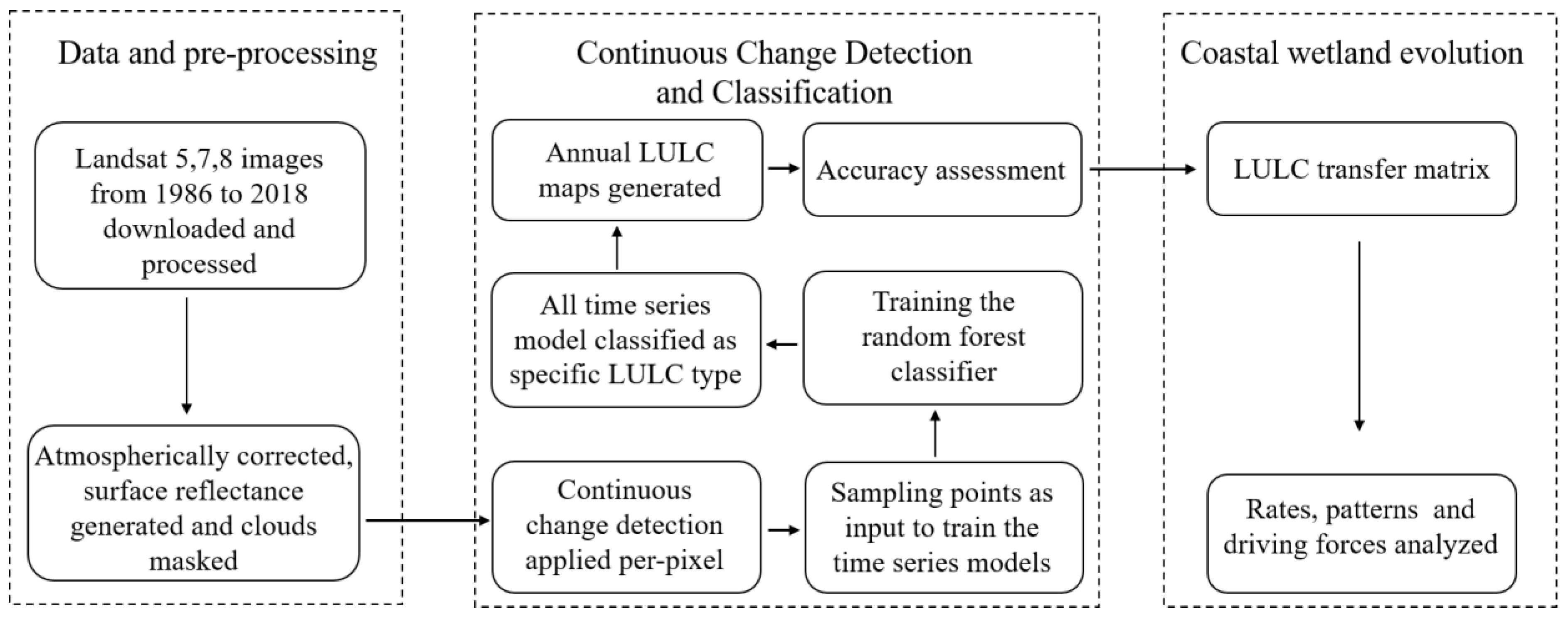
2.2. Data Preparation and the CCDC Algorithm
2.2.1. Data Acquisition and Preprocessing
2.2.2. The CCDC Algorithm and Its Implementation
2.3. Accuracy Assessment
3. Results
3.1. Thematic Classification Characterization
3.2. Changes of Coastal Wetlands in the LRE Area
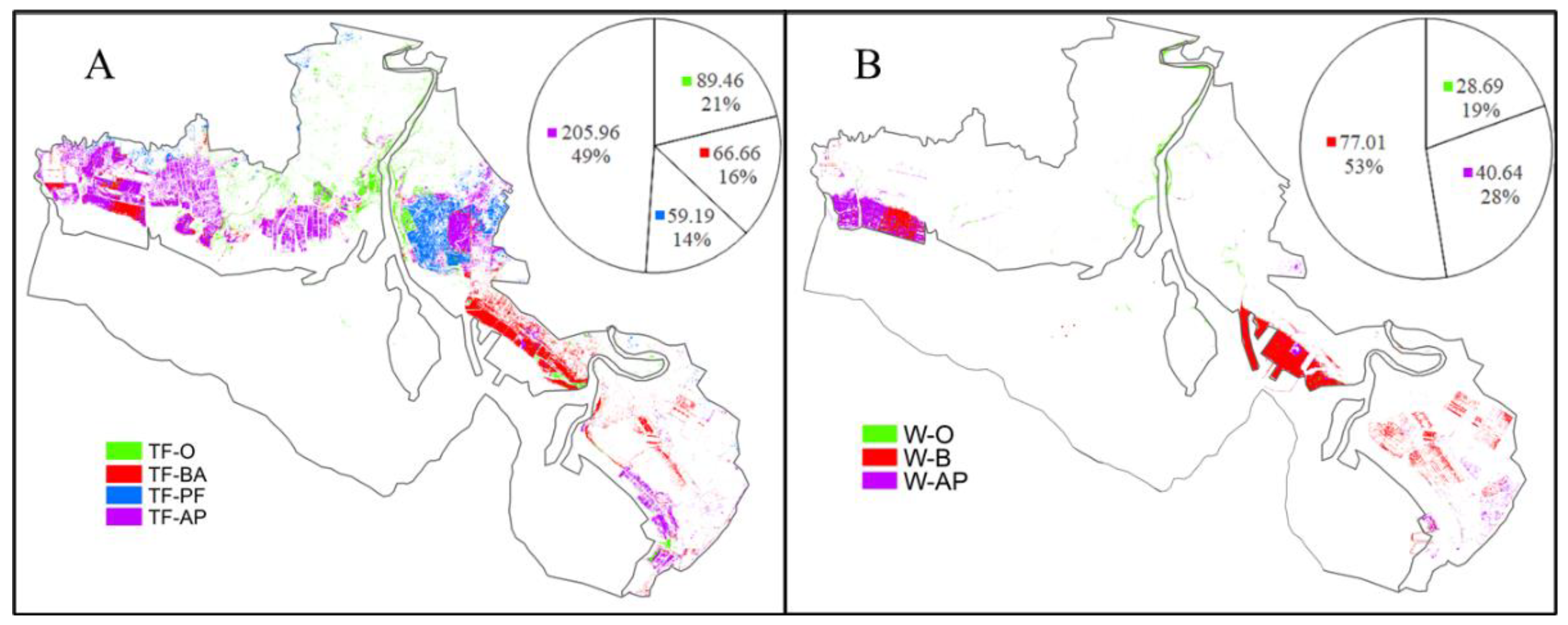
3.3. Spatial–Temporal Dynamics of Coastal Wetlands
3.3.1. Vegetated Coastal Wetlands
3.3.2. Tidal Flats and Shallow Marine Water
3.4. Existence Time of Vegetated Coastal Wetlands
4. Discussion
4.1. Driving Forces of Coastal Wetland Changes
4.1.1. Seepweed
4.1.2. Reeds
4.1.3. Tidal Flats and Shallow Marine Water
4.2. Planning and Conservation
4.3. Advantages and Limitations
5. Conclusions
Author Contributions
Funding
Data Availability Statement
Acknowledgments
Conflicts of Interest
References
- Jiang, T.-T.; Pan, J.-F.; Pu, X.-M.; Wang, B.; Pan, J.-J. Current status of coastal wetlands in China: Degradation, restoration, and future management. Estuar. Coast. Shelf Sci. 2015, 164, 265–275. [Google Scholar] [CrossRef]
- Mao, D.; Wang, Z.; Du, B.; Li, L.; Tian, Y.; Jia, M.; Zeng, Y.; Song, K.; Jiang, M.; Wang, Y. National wetland mapping in China: A new product resulting from object-based and hierarchical classification of Landsat 8 OLI images. ISPRS J. Photogramm. Remote Sens. 2020, 164, 11–25. [Google Scholar] [CrossRef]
- Ewers Lewis, C.J.; Baldock, J.A.; Hawke, B.; Gadd, P.S.; Zawadzki, A.; Heijnis, H.; Jacobsen, G.E.; Rogers, K.; Macreadie, P.I. Impacts of land reclamation on tidal marsh ‘blue carbon’ stocks. Sci. Total Environ. 2019, 672, 427–437. [Google Scholar] [CrossRef]
- Sun, Z.; Sun, W.; Tong, C.; Zeng, C.; Yu, X.; Mou, X. China’s coastal wetlands: Conservation history, implementation efforts, existing issues and strategies for future improvement. Environ. Int. 2015, 79, 25–41. [Google Scholar] [CrossRef]
- Yang, H.; Ma, M.; Thompson, J.R.; Flower, R.J. Protect coastal wetlands in China to save endangered migratory birds. Proc. Natl. Acad. Sci. USA 2017, 114, 5491–5492. [Google Scholar] [CrossRef] [Green Version]
- Luisa Martínez, M.; Mendoza-González, G.; Silva-Casarín, R.; Mendoza-Baldwin, E. Land use changes and sea level rise may induce a “coastal squeeze” on the coasts of Veracruz, Mexico. Glob. Environ. Chang. 2014, 29, 180–188. [Google Scholar] [CrossRef]
- Lin, Q.; Yu, S. Losses of natural coastal wetlands by land conversion and ecological degradation in the urbanizing Chinese coast. Sci. Rep. 2018, 8, 15046–15056. [Google Scholar] [CrossRef]
- Chen, L.; Ren, C.; Zhang, B.; Li, L.; Wang, Z.; Song, K. Spatiotemporal Dynamics of Coastal Wetlands and Reclamation in the Yangtze Estuary During Past 50 Years (1960s–2015). Chin. Geogr. Sci. 2018, 28, 386–399. [Google Scholar] [CrossRef] [Green Version]
- Zhao, Q.; Bai, J.; Huang, L.; Gu, B.; Lu, Q.; Gao, Z. A review of methodologies and success indicators for coastal wetland restoration. Ecol. Indic. 2016, 60, 442–452. [Google Scholar] [CrossRef]
- Meng, G.; Jing, L.; Chunlei, S.; Jiawei, X.; Li, W. A Review of Wetland Remote Sensing. Sensors 2017, 17, 777. [Google Scholar] [CrossRef] [Green Version]
- Qureshi, S.; Alavipanah, S.K.; Konyushkova, M.; Mijani, N.; Fathololomi, S.; Firozjaei, M.K.; Homaee, M.; Hamzeh, S.; Kakroodi, A.A. A Remotely Sensed Assessment of Surface Ecological Change over the Gomishan Wetland, Iran. Remote Sens. 2020, 12, 2989. [Google Scholar] [CrossRef]
- Wang, X.; Gao, X.; Zhang, Y.; Fei, X.; Chen, Z.; Wang, J.; Zhang, Y.; Lu, X.; Zhao, H. Land-Cover Classification of Coastal Wetlands Using the RF Algorithm for Worldview-2 and Landsat 8 Images. Remote Sens. 2019, 11, 1927. [Google Scholar] [CrossRef] [Green Version]
- Jin, H.; Huang, C.; Lang, M.W.; Yeo, I.-Y.; Stehman, S.V. Monitoring of wetland inundation dynamics in the Delmarva Peninsula using Landsat time-series imagery from 1985 to 2011. Remote Sens. Environ. 2017, 190, 26–41. [Google Scholar] [CrossRef] [Green Version]
- Di Vittorio, C.A.; Georgakakos, A.P. Land cover classification and wetland inundation mapping using MODIS. Remote Sens. Environ. 2018, 204, 1–17. [Google Scholar] [CrossRef]
- Mahdianpari, M.; Salehi, B.; Mohammadimanesh, F.; Brisco, B.; Mahdavi, S.; Amani, M.; Granger, J.E. Fisher Linear Discriminant Analysis of coherency matrix for wetland classification using PolSAR imagery. Remote Sens. Environ. 2018, 206, 300–317. [Google Scholar] [CrossRef]
- Chen, S.; Ma, A.; Li, Z. Landscape Pattern Changes and Its Driving Mechanism of the Wetland in Liaohe. Chin. J. Eco-Agric. 2011, 19, 468–476. [Google Scholar]
- Yang, T.; Guan, X.; Qian, Y.; Xing, W.; Wu, H. Efficiency Evaluation of Urban Road Transport and Land Use in Hunan Province of China Based on Hybrid Data Envelopment Analysis (DEA) Models. Sustainability 2019, 11, 3826. [Google Scholar] [CrossRef] [Green Version]
- Wu, W.; Zhao, S.; Zhu, C.; Jiang, J. A comparative study of urban expansion in Beijing, Tianjin and Shijiazhuang over the past three decades. Landsc. Urban Plan. 2015, 134, 93–106. [Google Scholar] [CrossRef]
- Kennedy, R.E.; Yang, Z.; Cohen, W.B. Detecting trends in forest disturbance and recovery using yearly Landsat time series: 1. LandTrendr—Temporal segmentation algorithms. Remote Sens. Environ. 2010, 114, 2897–2910. [Google Scholar] [CrossRef]
- Huang, C.; Goward, S.N.; Masek, J.G.; Thomas, N.; Zhu, Z.; Vogelmann, J.E. An automated approach for reconstructing recent forest disturbance history using dense Landsat time series stacks. Remote Sens. Environ. 2010, 114, 183–198. [Google Scholar] [CrossRef]
- Zhu, Z.; Woodcock, C.E. Continuous change detection and classification of land cover using all available Landsat data. Remote Sens. Environ. 2014, 144, 152–171. [Google Scholar] [CrossRef] [Green Version]
- Zhu, Z.; Zhou, Y.; Seto, K.C.; Stokes, E.C.; Deng, C.; Pickett, S.T.A.; Taubenböck, H. Understanding an urbanizing planet: Strategic directions for remote sensing. Remote Sens. Environ. 2019, 228, 164–182. [Google Scholar] [CrossRef]
- Awty-Carroll, K.; Bunting, P.; Hardy, A.; Bell, G. Using Continuous Change Detection and Classification of Landsat Data to Investigate Long-Term Mangrove Dynamics in the Sundarbans Region. Remote Sens. 2019, 11, 2833. [Google Scholar] [CrossRef] [Green Version]
- Tian, Y.; Luo, L.; Mao, D.; Wang, Z.; Li, L.; Liang, J. Using Landsat images to quantify different human threats to the Shuangtai Estuary Ramsar site, China. Ocean Coast. Manag. 2017, 135, 56–64. [Google Scholar] [CrossRef]
- Ma, C.; Ye, S.; Lin, T.; Ding, X.; Yuan, H.; Guo, Z. Source apportionment of polycyclic aromatic hydrocarbons in soils of wetlands in the Liao River Delta, Northeast China. Mar. Pollut. Bull. 2014, 80, 160–167. [Google Scholar] [CrossRef] [PubMed]
- Gao, X.; Zhang, Y.; Ding, S.; Zhao, R.; Meng, W. Response of fish communities to environmental changes in an agriculturally dominated watershed (Liao River Basin) in northeastern China. Ecol. Eng. 2015, 76, 130–141. [Google Scholar] [CrossRef]
- Hansen, M.C.; Loveland, T.R. A review of large area monitoring of land cover change using Landsat data. Remote Sens. Environ. 2012, 122, 66–74. [Google Scholar] [CrossRef]
- Claverie, M.; Vermote, E.F.; Franch, B.; Masek, J.G. Evaluation of the Landsat-5 TM and Landsat-7 ETM+ surface reflectance products. Remote Sens. Environ. 2015, 169, 390–403. [Google Scholar] [CrossRef]
- Zhu, Z.; Gallant, A.L.; Woodcock, C.E.; Pengra, B.; Olofsson, P.; Loveland, T.R.; Jin, S.; Dahal, D.; Yang, L.; Auch, R.F. Optimizing selection of training and auxiliary data for operational land cover classification for the LCMAP initiative. ISPRS J. Photogramm. Remote Sens. 2016, 122, 206–221. [Google Scholar] [CrossRef] [Green Version]
- Zhu, Z.; Wang, S.; Woodcock, C.E. Improvement and expansion of the Fmask algorithm: Cloud, cloud shadow, and snow detection for Landsats 4–7, 8, and Sentinel 2 images. Remote Sens. Environ. 2015, 159, 269–277. [Google Scholar] [CrossRef]
- Berhane, T.M.; Lane, C.R.; Mengistu, S.G.; Christensen, J.; Golden, H.E.; Qiu, S.; Zhu, Z.; Wu, Q. Land-Cover Changes to Surface-Water Buffers in the Midwestern USA: 25 Years of Landsat Data Analyses (1993–2017). Remote Sens. 2020, 12, 754. [Google Scholar] [CrossRef] [Green Version]
- Pontius, R.G.; Millones, M. Death to Kappa: Birth of quantity disagreement and allocation disagreement for accuracy assessment. Int. J. Remote Sens. 2011, 32, 4407–4429. [Google Scholar] [CrossRef]
- Foody, G.M. Status of land cover classification accuracy assessment. Remote Sens. Environ. 2002, 80, 185–201. [Google Scholar] [CrossRef]
- Wang, Y.; Ji, Y.; Sun, Z.; Li, J.; Zhang, M.; Wu, G. Analysis of Suaeda heteroptera cover change and its hydrology driving factors in the Liao River Estuary wetlands, China. IOP Conf. Ser. Earth Environ. Sci. 2020, 467, 12150–12158. [Google Scholar] [CrossRef] [Green Version]
- Yang, Y.; Chang, Y.; Hu, Y.; Liu, M.; Li, Y. Application of small remote sensing satellite constellations for environmental hazards in wetland landscape mapping: Taking Liaohe Delta, Liaoning Province of Northeast China as a case. Ying Yong Sheng Tai Xue Bao 2011, 22, 1552–1558. [Google Scholar]
- Lu, W.; Xiao, J.; Lei., W.; Du., J.; Li, Z.; Cong, P.; Hou, W.; Zhang, J.; Chen, L.; Zhang, Y.; et al. Human activities accelerated the degradation of saline seepweed red beaches by amplifying top-down and bottom-up forces. Ecosphere 2018, 9, 2352–2371. [Google Scholar] [CrossRef] [Green Version]
- Liu, X.; Ke, L.; Zhuang, H.; Yang, X.; Song, N.; Wang, S. Analysis of Coupling Co-Ordination between Intensive Sea Use and the Marine Economy in the Liaoning Coastal Economic Belt of China. Complexity 2020, 2020, 1–13. [Google Scholar] [CrossRef]
- Nan, S. Liao river basin of Liaoning tourism development discussed. Territ. Nat. Resour. Study 2015, 25, 71–73. [Google Scholar]
- Oleśniewicz, P.; Pytel, S.; Markiewicz-Patkowska, J.; Szromek, A.R.; Jandová, S. A Model of the Sustainable Management of the Natural Environment in National Parks—A Case Study of National Parks in Poland. Sustainability 2020, 12, 2704. [Google Scholar] [CrossRef] [Green Version]
- Liu, M.; Liu, S.; Ning, Y.; Zhu, Y.; Valbuena, R.; Guo, R.; Li, Y.; Tang, W.; Mo, D.; Rosa, I.M.D.; et al. Co-Evolution of Emerging Multi-Cities: Rates, Patterns and Driving Policies Revealed by Continuous Change Detection and Classification of Landsat Data. Remote Sens. 2020, 12, 2905. [Google Scholar] [CrossRef]
- Zhu, Z.; Woodcock, C.E.; Holden, C.; Yang, Z. Generating synthetic Landsat images based on all available Landsat data: Predicting Landsat surface reflectance at any given time. Remote Sens. Environ. 2015, 162, 67–83. [Google Scholar] [CrossRef]
- Tang, W.; Liu, S.; Kang, P.; Peng, X.; Li, Y.; Guo, R.; Jia, J.; Liu, M.; Zhu, L. Quantifying the lagged effects of climate factors on vegetation growth in 32 major cities of China. Ecol. Indic. 2021, 132, 108290. [Google Scholar] [CrossRef]
- Jia, M.; Wang, Z.; Liu, D.; Ren, C.; Tang, X.; Dong, Z. Monitoring Loss and Recovery of Salt Marshes in the Liao River Delta, China. J. Coast. Res. 2015, 300, 371–377. [Google Scholar] [CrossRef]
- Osland, M.J.; Spivak, A.C.; Nestlerode, J.A.; Lessmann, J.M.; Almario, A.E.; Heitmuller, P.T.; Russell, M.J.; Krauss, K.W.; Alvarez, F.; Dantin, D.D.; et al. Ecosystem Development After Mangrove Wetland Creation: Plant–Soil Change Across a 20-Year Chronosequence. Ecosystems 2012, 15, 848–866. [Google Scholar] [CrossRef]
- VanRees-Siewert, K.L.; Dinsmore, J.J. Infuence of Wetland Age on Bird Use of Restored Wetlands in Iowa. Wetlands 1996, 16, 577–582. [Google Scholar] [CrossRef]
- Anish, D.; Kanwaljit, K. Age and growth patterns in Channa marulius from Harike Wetland (A Ramsar site), Punjab, India. J. Environ. Biol. 2006, 27, 377–380. [Google Scholar]
- Wolf, K.L.; Ahn, C.; Noe, G.B. Development of Soil Properties and Nitrogen Cycling in Created Wetlands. Wetlands 2011, 31, 699–712. [Google Scholar] [CrossRef]
- Ahn, C.; Jones, S. Assessing Organic Matter and Organic Carbon Contents in Soils of Created Mitigation Wetlands in Virginia. Environ. Eng. Res. 2013, 18, 151–156. [Google Scholar] [CrossRef]


| SH | BA | FL | PA | PF | TF | SMW | AP | Total | User’s accuracy | |
| SH | 91 | 2 | 0 | 0 | 0 | 3 | 1 | 4 | 101 | 0.90 |
| BA | 3 | 989 | 29 | 37 | 21 | 63 | 18 | 144 | 1304 | 0.76 |
| FL | 0 | 3 | 27 | 4 | 4 | 0 | 0 | 0 | 38 | 0.71 |
| PA | 2 | 40 | 1 | 1241 | 67 | 13 | 9 | 21 | 1394 | 0.89 |
| PF | 0 | 19 | 2 | 14 | 379 | 2 | 0 | 12 | 428 | 0.89 |
| TF | 23 | 33 | 0 | 7 | 0 | 893 | 50 | 96 | 1102 | 0.81 |
| SMW | 1 | 4 | 0 | 4 | 0 | 137 | 4146 | 73 | 4365 | 0.95 |
| AP | 0 | 73 | 0 | 15 | 1 | 52 | 23 | 1003 | 1167 | 0.86 |
| Total | 120 | 1163 | 59 | 1322 | 472 | 1163 | 4247 | 1353 | 9899 | |
| Producer’s accuracy | 0.76 | 0.85 | 0.46 | 0.94 | 0.80 | 0.77 | 0.98 | 0.74 | 0.88 |
Publisher’s Note: MDPI stays neutral with regard to jurisdictional claims in published maps and institutional affiliations. |
© 2021 by the authors. Licensee MDPI, Basel, Switzerland. This article is an open access article distributed under the terms and conditions of the Creative Commons Attribution (CC BY) license (https://creativecommons.org/licenses/by/4.0/).
Share and Cite
Peng, J.; Liu, S.; Lu, W.; Liu, M.; Feng, S.; Cong, P. Continuous Change Mapping to Understand Wetland Quantity and Quality Evolution and Driving Forces: A Case Study in the Liao River Estuary from 1986 to 2018. Remote Sens. 2021, 13, 4900. https://doi.org/10.3390/rs13234900
Peng J, Liu S, Lu W, Liu M, Feng S, Cong P. Continuous Change Mapping to Understand Wetland Quantity and Quality Evolution and Driving Forces: A Case Study in the Liao River Estuary from 1986 to 2018. Remote Sensing. 2021; 13(23):4900. https://doi.org/10.3390/rs13234900
Chicago/Turabian StylePeng, Jianwei, Shuguang Liu, Weizhi Lu, Maochou Liu, Shuailong Feng, and Pifu Cong. 2021. "Continuous Change Mapping to Understand Wetland Quantity and Quality Evolution and Driving Forces: A Case Study in the Liao River Estuary from 1986 to 2018" Remote Sensing 13, no. 23: 4900. https://doi.org/10.3390/rs13234900