Article

Estimation of Vertical Fuel Layers in Tree Crowns Using High Density LiDAR Data

1
Integrated Remote Sensing Studio, Department of Forest Resources Management, University of British Columbia, Vancouver, BC V6T 1Z4, Canada
2
Tree Ring Lab, Department of Forest and Conservation Sciences, University of British Columbia, Vancouver, BC V6T 1Z4, Canada
3
FYBR Solutions Inc., 211 E Georgia St #305, Vancouver, BC V6A 1Z6, Canada
*
Author to whom correspondence should be addressed.
Remote Sens. 2021, 13(22), 4598; https://doi.org/10.3390/rs13224598
Submission received: 29 September 2021 / Revised: 8 November 2021 / Accepted: 11 November 2021 / Published: 16 November 2021
(This article belongs to the Special Issue Advances in Forest Fire Behaviour Modelling Using Remote Sensing)

Abstract

:
The accurate prediction and mitigation of wildfire behaviour relies on accurate estimations of forest canopy fuels. New techniques to collect LiDAR point clouds from remotely piloted aerial systems (RPAS) allow for the prediction of forest fuels at extremely fine scales. This study uses a new method to examine the ability of such point clouds to characterize the vertical arrangement and volume of crown fuels from within individual trees. This method uses the density and vertical arrangement of LiDAR points to automatically extract and measure the dimensions of each cluster of vertical fuel. The amount and dimensions of these extracted clusters were compared against manually measured clusters that were collected through the manual measurement of over 100 trees. This validation dataset was composed of manual point cloud measurements for all portions of living crown fuel for each tree. The point clouds used for this were ground-based LiDAR point clouds that were ~80 times denser than the RPAS LiDAR point clouds. Over 96% of the extracted clusters were successfully matched to a manually measured cluster, representing ~97% of the extracted volume. A smaller percentage of the manually measured clusters (~79%) were matched to an extracted cluster, although these represented ~99% of the total measured volume. The vertical arrangement and dimensions of the matched clusters corresponded strongly to one another, although the automated method generally overpredicted each cluster’s lower boundary. Tree-level volumes and crown width were, respectively, predicted with R-squared values of 0.9111 and 0.7984 and RMSE values of 44.36 m2 and 0.53 m. Weaker relationships were observed for tree-level metrics that relied on the extraction of lower crown features (live crown length, live crown base height, lowest live branch height). These metrics were predicted with R-squared values of 0.5568, 0.3120, and 0.2011 and RMSE values of 3.53 m, 3.55 m, and 3.66 m. Overall, this study highlights strengths and weaknesses of the developed method and the utility of RPAS LiDAR point clouds relative to ground-based point clouds.

Graphical Abstract

1. Introduction

While wildfires are critical disturbances that can help to maintain the health and diversity of a variety of ecosystems [1], changes in global fire regimes are projected to have severe and long-lasting ecological repercussions. Depending on the particular geographic area, these changes include increases in fire frequency, size, and intensity and can be attributed to climate change, fire suppression, and changes in vegetation composition [2]. Departures from historic fire regimes are projected to cause many forested ecosystems to have reductions in ecosystem resilience, a reduced capacity to provide ecosystem services, and to experience shifts in forest structure and composition [3]. These changing fire regimes have already had substantial, multi-faceted socio-economic impacts, such as active suppression costs, damage to infrastructure, as well as short- and long-term impacts to human health [4]. A recent literature review estimated the total economic burden of wildfire in the United States alone to be more than $71.1 billion per year [4].
To evaluate and mitigate the risks associated with wildfires, land managers make use of an array of wildfire behaviour models. These models predict potential fire behaviour using site-specific information about weather, topography, and fuels [5]. Of the required fuel information, significant attention has been given to forest canopy fuels. Accurate measurements of canopy fuels are critical, as they are the primary fuel layer that supports the initiation and spread of crown fire [6]. These measurements are typically derived from field-collected forest inventory data using allometric equations that produce stand-level fuel metrics [5,7]. The derivation of these critical metrics begins at the individual tree-level with an estimation of the amount and vertical arrangement of combustible fuels within individual tree crowns. This is typically calculated by deriving the total weight of crown foliage and fine fuels and distributing them from the base of the crown to the treetop [5,7].
While this approach is widely used in a variety of wildfire behaviour and fuel models, there are well-known limitations. First, the allometric equations assume that crown fuels are uniformly distributed within individual trees and do not typically incorporate any measure of crown width [8]. This is an oversimplification that has been shown to impact fire behaviour [9]. Additionally, due to the high cost of developing local allometries, generic equations are commonly applied, potentially resulting in unreliable predictions [10,11]. The second limitation revolves around the critical measure of live crown base height. This metric is used as the starting height to vertically distribute crown fuel, as well as to estimate the likelihood of fire propagating from the surface into tree crowns [12]. Due to vague and differing definitions, this metric can be difficult to consistently measure in the field. Variation in this definition relates to how different authors define lower crown layers, the primary crown, and the vertical continuity between them. Early research did not always specify continuity and often defined live crown base height as the height of the lowest live branch [13]. Others offer more detail and necessitate that these branches must provide a vertically continuous path into the primary crown [14]. Even more detailed definitions followed, refining continuity by specifying that vertical gaps of up to ~1.5 m can exist within a “continuous” crown [15].
Improving the estimation of crown fuels is an active area of research, although much of this research relies solely on field-based methods. While these studies are valuable, their applications are typically limited to relatively fine spatial scales. Alternatively, high density three-dimensional light detection and ranging (LiDAR) point clouds have been used to estimate tree- and stand-level fuel metrics. For over a decade, LiDAR point clouds acquired from conventional aircraft have been successfully used to estimate broad scale, stand-level canopy fuel metrics [16,17,18]. Recently, more detailed and comprehensive characterizations of tree-level crown fuel have been undertaken using terrestrial or mobile laser scanning (TLS or MLS, respectively) [19,20,21,
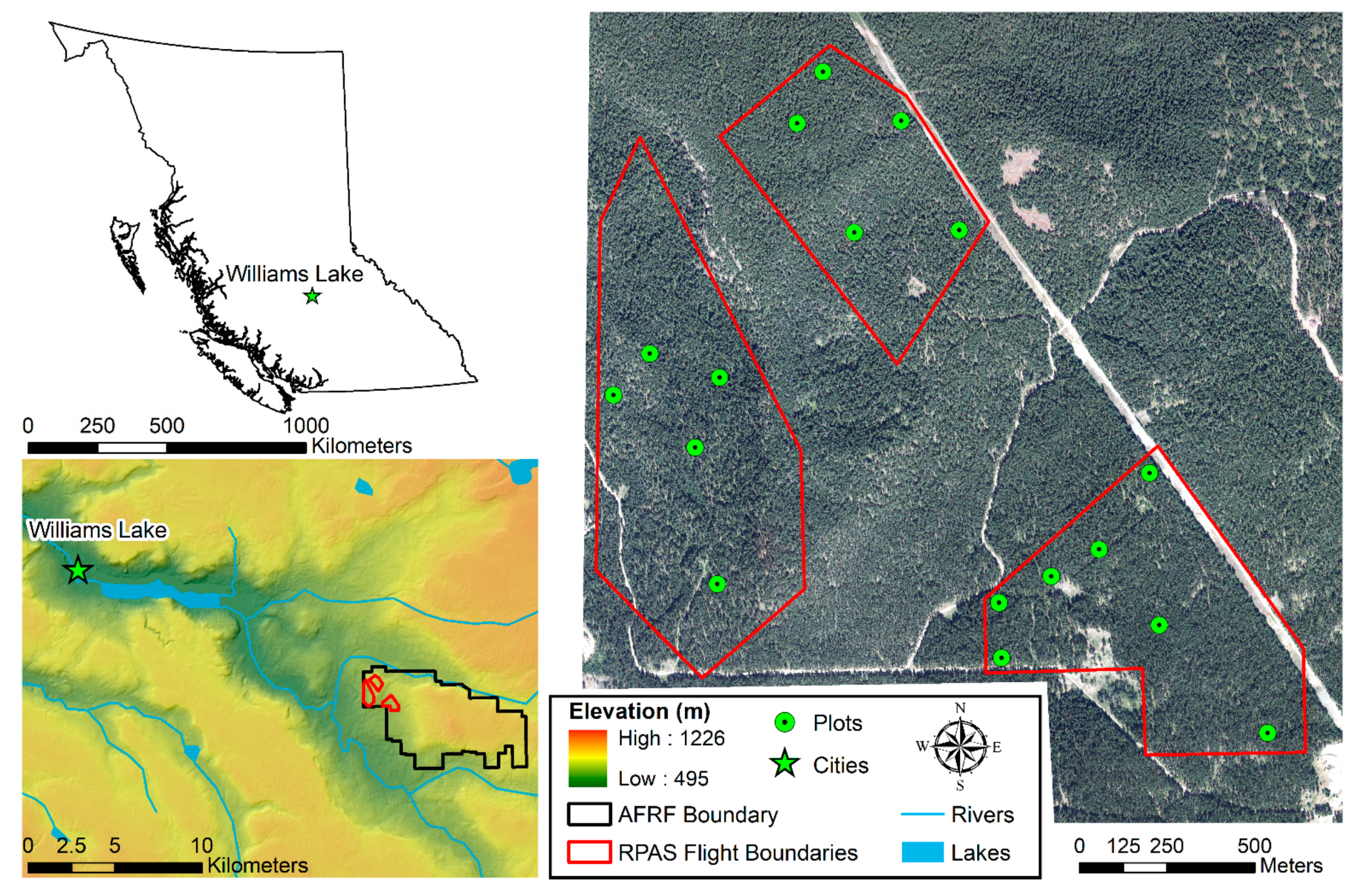
22]. The past five years has seen the acquisition of high-density LiDAR point clouds from remotely piloted aerial systems (RPAS). These types of point clouds can capture greater levels of detail than conventional aircraft-acquired LiDAR. These point clouds are not as dense as TLS or MLS point clouds but offer much greater spatial coverage. These characteristics result in RPAS LiDAR point clouds having the potential to characterize crown fuels at comparable detail to TLS but across broader spatial scales.
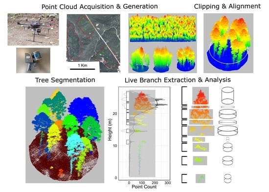
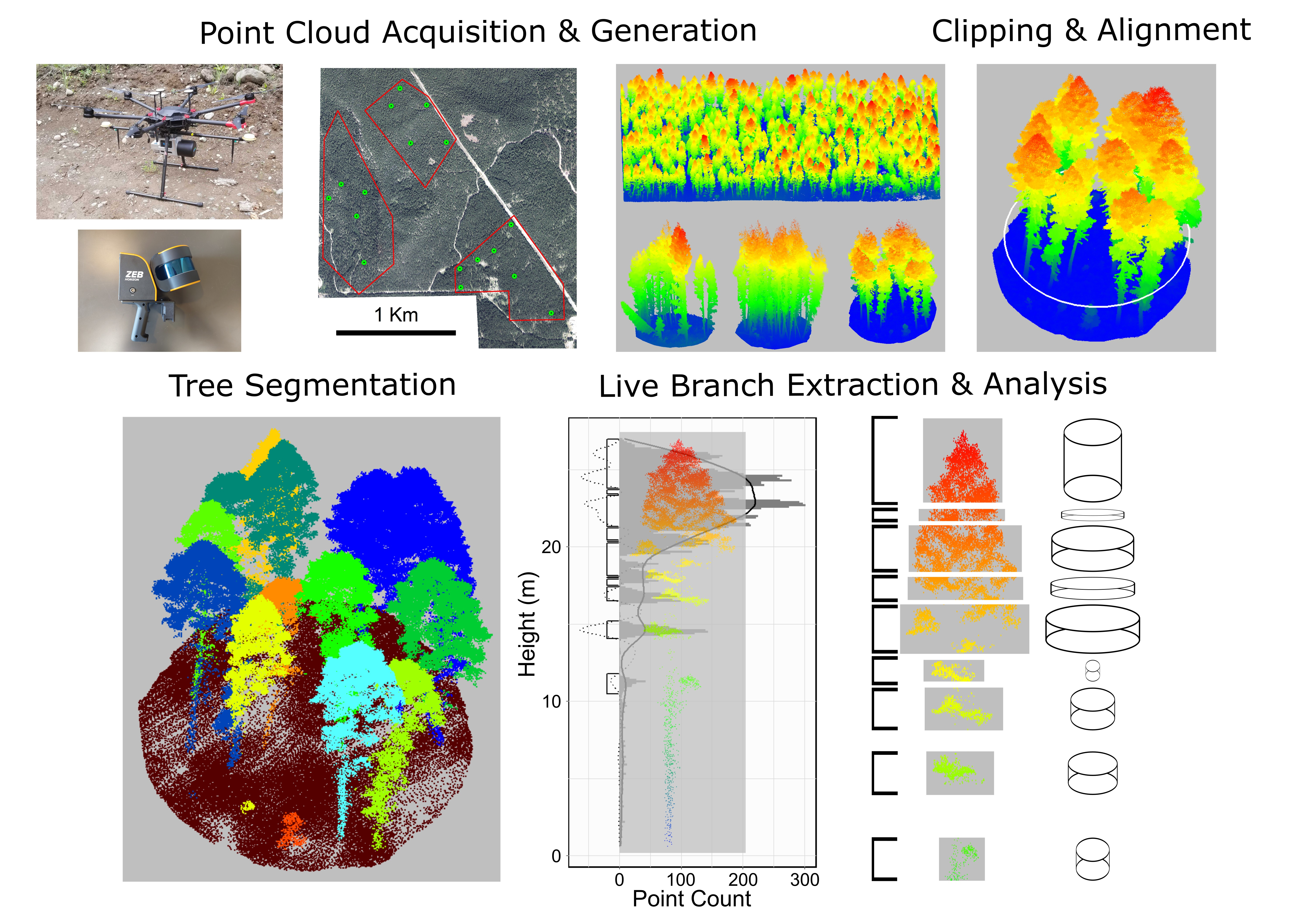
In this study, we examine the capability of high-density RPAS point clouds to characterize the vertical arrangement and volume of live crown fuels within individual trees. To accomplish this, we develop an automated method that detects and quantifies all branch structures that contain live foliage, hereafter “live branch clusters”. We apply our new method to over 100 individual trees with varying crown fuel loads from a dry, interior British Columbia forest system. Comparisons were made against manual measurements taken from MLS point clouds. The vertical arrangement of crown fuel is then summarized at the tree-level to describe crown fuel metrics in a comprehensive and systematic way. Using this approach, the amount and distribution of crown fuel can be accurately mapped across large numbers of trees, providing key fuel inputs for fire behaviour models.
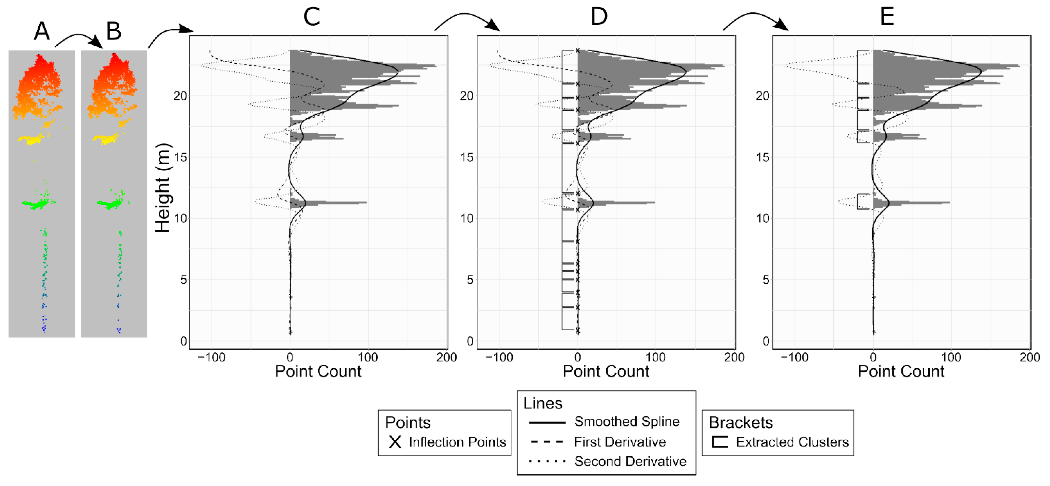
2. Materials and Methods

2.1. Study Area

The study area is located approximately 20 km south-east of Williams Lake, British Columbia, in the Knife Creek portion of the Alex Fraser Research Forest (AFRF) (Figure 1). This portion of the AFRF is part of the Interior Douglas-fir biogeoclimatic zone and is almost entirely composed of interior Douglas-fir (Pseudotsuga menziesii var. glauca). While not present within our sampled plots, hybrid white spruce (Picea engelmannii X Picea glauca) and trembling aspen (Populus tremuloides) can also be found in the area [23]. In recent decades, the forest has been affected by western spruce budworm (Choristoneura occidentalis Freeman) and Douglas-fir bark beetle (Dendroctonus pseudotsugae Hopkins) but has not burned [24]. As part of a long-term experiment, three forest stands were partially harvested in 1984 and 2014. This harvesting was performed to promote a diverse forest structure of uneven-aged clumps of trees interspersed with small canopy openings. Throughout the experiment, permanent sample plots are distributed at 100 m intervals forming a uniform grid. In each of the three forest stands, five to seven plots were selected to represent a range of treatments, topography, and forest structures. In total, we collected plot- and stand-level remotely sensed data across 17 plots.

2.2. Remote Sensing Data Acquisition

The RPAS and ground-based LiDAR point clouds were collected over three days in July and September of 2019. The RPAS LiDAR point clouds were acquired using a GreenValley LiAir S200 LiDAR system with a relative system accuracy of ±5 cm. The ground-based LiDAR point clouds, hereafter referred to as mobile laser scanning (MLS) point clouds, were collected for validation purposes using a handheld GeoSLAM HORIZON system. This system has a relative accuracy of ± 3 cm and collects extremely dense LiDAR point clouds from beneath the canopy using the simultaneous localization and mapping (SLAM) algorithm. This method allows the system to collect data while in motion, reducing errors of occlusion that are common with most tripod-mounted TLS systems [25].
The RPAS LiDAR was acquired using a DJI Matrice 600 equipped with a real-time kinematic (RTK) GPS system. The RPAS was flown at a consistent 80 m above ground level across the three stands. The hardware and flight parameters allowed the point clouds to be produced at ~535 points/m2 and georeferenced at an absolute accuracy of ±2 cm. The MLS data was collected for each of the 17 plots by having an operator activate the GeoSLAM Horizon at plot center and walk in an outwardly expanding spiral. This was performed in a way that ensured each spiral was spaced ~3 m apart, with the final spiral being ~15 m away from plot center. This process resulted in the entire 11.28 m radius plot having LiDAR points taken from all sides with an average point density of ~42,000 points/m2. Examples of each type of point clouds can be seen in Figure 2.

2.3. Methods

Our method consists of four steps: initial point cloud processing and individual tree segmentation, live branch cluster extraction and analysis, validation, and accuracy assessment.

2.3.1. Point Cloud Processing and Individual Tree Segmentation

The GeoSLAM point clouds were aligned to the RPAS LiDAR point clouds, as the initial clouds were not georeferenced to a datum. This alignment was carried out using the iterative closest point (ICP) algorithm [26], as follows. The ICP algorithm requires both point clouds to be approximately aligned before applying. To carry this out, the RPAS LiDAR point clouds were clipped to 30 m radius circles, with each representing a buffered plot. The clipped RPAS LiDAR point clouds were then used as a guide to manually shift the MLS point clouds so that both point clouds overlapped one another. The RPAS LiDAR point clouds were then used as a reference to precisely align and spatially register the MLS point clouds. Points that were duplicated or considered outliers were removed. All remaining points were classified as either ground or non-ground and normalized relative to ground height.
Non-ground RPAS LiDAR point clouds were segmented into individual trees using a point-based segmentation algorithm [27]. This algorithm uses a top-down approach that takes the highest point as the seed point for the first tree. Additional points are then added according to a series of point addition rules. The first segmentation is considered complete when all candidate points have been considered, after which the segmented points are assigned a tree ID. The process is then repeated for the rest of the point cloud [27]. This algorithm is generally considered to be among the most accurate routines, but segmentation accuracy is variable depending on tree density, topography, and crown classes [27,28,29]. To ensure the developed method was not influenced by poorly or incorrectly segmented tree crowns, the following steps were carried out. Each segmented tree was visually assessed, and any tree that was not completely segmented or included points from neighboring trees was removed. The boundaries of the suitable segmentations were then used to segment the MLS point clouds, which were then solely used for the accuracy assessment.

2.3.2. Live Branch Cluster Extraction and Analysis

Once individual trees had been extracted, the locations and dimensions of live branch clusters were estimated using a new approach developed for this study (Figure 3). This approach was applied separately to each tree through three key steps. First, the segmented point cloud was simplified using an alpha shape-based point cloud thinning method. In the context of point clouds, an alpha shape refers to a three-dimensional polygon that is draped over a set of points. This polygon is then used to classify each point depending on where it falls relative to the polygon. This characterization can be performed at a variable level of detail depending on a user specified alpha parameter, with low alpha parameter values being used to construct extremely detailed shapes and infinite alpha parameter values being used to construct three-dimensional convex hulls [30]. A very fine alpha parameter was used to calculate a detailed alpha shape for each tree segment. Any points that did not fall on the outside of this three-dimensional shape were then removed. The removal of these points reduced the size of each point cloud while maintaining points that are likely to represent living and fine fuels on outer portions of branches.
The second step of this approach used the remaining points to estimate the lower and upper boundaries of all live branch clusters. This was accomplished by characterizing the vertical distribution of points. The characterization involved the calculation of histograms and the extraction of inflection points, partially following methods laid out in [31]. These histograms were created based on the number of points within each 10 cm vertical portion of the tree. A smoothed spline was then calculated that followed a relatively detailed shape of the histogram. The first two derivatives of the spline were then derived and used to calculate inflection points, defined as the heights that the second derivative values were equal to zero. To ensure that the highest portion of live crown was included, an additional upper cluster boundary was added to each tree’s maximum point height. Through this process, the boundaries of live branch clusters were initially defined. These initial clusters included some portions of the tree devoid of living fuel, which were eliminated by removing clusters that had average point counts and first derivative values below a threshold. The same threshold was applied to all initial clusters across the analyzed trees.
The final step of this approach involved the calculation of the following metrics for each live branch cluster: total vertical length, diameter, and three-dimensional volume. The total vertical length of each cluster was calculated by subtracting the upper and lower boundaries. The diameter and volume of each cluster was calculated from the segmented point cloud, using the following method. The lower and upper boundary of each cluster was used to extract the portion of the relevant point cloud. This extracted portion was then used to calculate diameter values across four equally spaced, intersecting axes. These values were then averaged to derive the cluster diameter. This diameter was then used with the cluster vertical length value to calculate cylindrical volumes of each cluster.
Branch-level metrics were then accumulated for each individual tree to describe the amount and arrangement of living branch clusters for each tree (Figure 4). These metrics included: the height of the lowest live branch cluster, defined as the lower boundary of the lowest extracted cluster; the total crown length, calculated using the sum of all vertical cluster lengths; the crown width, defined as the maximum cluster diameter; and the total live branch volume, calculated by taking the sum of all individual cluster volumes. In addition to these metrics, live crown base height was calculated by merging all extracted clusters that had upper and lower boundaries within 25 cm of each other. The lower boundary of the highest merged cluster was then used as the live crown base height.

2.3.3. Validation Data Collection

All vertically continuous branch clusters that visibly contained live foliage were manually measured by a trained interpreter using the MLS point clouds. To do so, the interpreter was provided with the segmented point clouds and instructed to measure all living branch clusters using a heads-up display. The following measurements were made for each cluster: lower height, upper height, and maximum diameter. These manually measured branch clusters were then accumulated for each individual tree using the same method as was used for the automated approach.

2.3.4. Accuracy Assessment

The accuracy assessment consisted of three steps: cluster matching, cluster-level validation, and tree-level validation. Clusters were characterized as either true positive (TP) matches, false positive (FP) misses, or false negative (FN) misses. Extracted clusters were considered TP if their midpoint was between the lower and upper boundary of a manually measured cluster and FP if their midpoint was not. Measured clusters were considered FN if there was no extracted cluster midpoint between their lower and upper boundaries. The cluster matching accuracy was evaluated using a standard error matrix, with overall accuracy, commission errors, and omission errors calculated according to the equations found below. A suite of statistics for each TP, FP, and FN cluster were calculated to compare the locations, sizes, and total volumes of each extracted and measured cluster.
Overall accuracy = (TP)/(TP + FP + FN)
Commission error = (FP)/(TP + FP + FN)
Omission error = (FN)/(TP + FP + FN)
Portions of vertically continuous fuel were commonly extracted as multiple, smaller clusters, instead of a single large cluster, as was typical of the validation data. This difference was a result of each dataset being collected with different goals in mind. The validation data were collected in a way that allowed a manual interpreter to efficiently measure all vertically continuous portions of live foliage. The automated method was designed to extract and quantify live branch clusters at finer levels of detail. These differences resulted in cases where multiple extracted clusters were matched with the same measured cluster. All these extracted clusters were still considered to be TP, as they successfully extracted portions of the tree that the trained interpreter found to contain live fuel. This differs from the definition of TP commonly used to describe tree-level segmentation accuracy used in most individual tree-detection studies [27]. In order to evaluate multiple extracted clusters against the one manually measured cluster, the extracted clusters were aggregated (Figure 5) in the following fashion. The lower and upper boundaries were, respectively, set to the lowest and highest cluster boundaries, which were used to recalculate vertical cluster length. The new cluster diameter was set equal to the maximum cluster diameter, which was used along with the new vertical cluster length to recalculate cluster volume. This aggregation simplified the extracted clusters by replicating the rules that the trained interpreter followed when collecting the validation data. By aggregating in this way, the strengths and weaknesses of the cluster metrics were able to be reliably assessed.
The cluster-level validation was carried out by building linear relationships between the metrics calculated from all the successfully matched extracted and measured clusters. The tree-level validation was carried out using the same method but using all the automatically extracted and manually measured tree-level metrics.

2.4. Software

The software used in this study is as follows. The RPAS LiDAR and MLS point clouds were, respectively, converted to laz file format using LiDAR360 (https://greenvalleyintl.com/?LiDAR360/, accessed on 15 November 2021) and GeoSLAM Hub software (https://geoslam.com/hub/, accessed on 15 November 2021). The ICP alignment and collection of validation data were completed using the open-source CloudCompare software [32]. All point cloud classification and cleaning were completed using LAStools [33]. The live branch cluster extractions were completed with the R statistical software (4.0.4) and the following packages: lidR [34,35], rLiDAR [36], and alphashape3d [37].

3. Results

Below, we present the following results: cluster matching, cluster-level validation, and tree-level validation. The cluster matching results show the degree to which the automatically extracted and manually measured clusters aligned with one another. The cluster-level results show the level of agreement between the dimensions and vertical arrangements of the successfully matched clusters, while the tree-level results show the level of agreement between the extracted and measured accumulated metrics for each tree.

3.1. Cluster Matching

Table 1 summarizes statistics for all extracted and measured clusters, as well as the overall accuracy and commission and omission errors. In general, the automated method extracted many more clusters than the validation method. The extracted and measured clusters had similar mean diameters, but the extracted clusters tended to have much lower vertical length and volume values. The majority of automatically extracted clusters were successfully matched to a manually measured cluster (797 of 825 clusters). This resulted in a high overall accuracy (91.72%) with a low commission error (3.2%). Only 44 measured clusters did not correspond to an extracted cluster, resulting in an omission error of 5.06%. The lower mean heights of the FN clusters relative to all measured clusters indicate that these erroneous clusters tended to be located lower in the tree. The low mean and total volumes additionally indicate that these cluster were smaller in size than other manually measured clusters.

3.2. Cluster-Level Validation

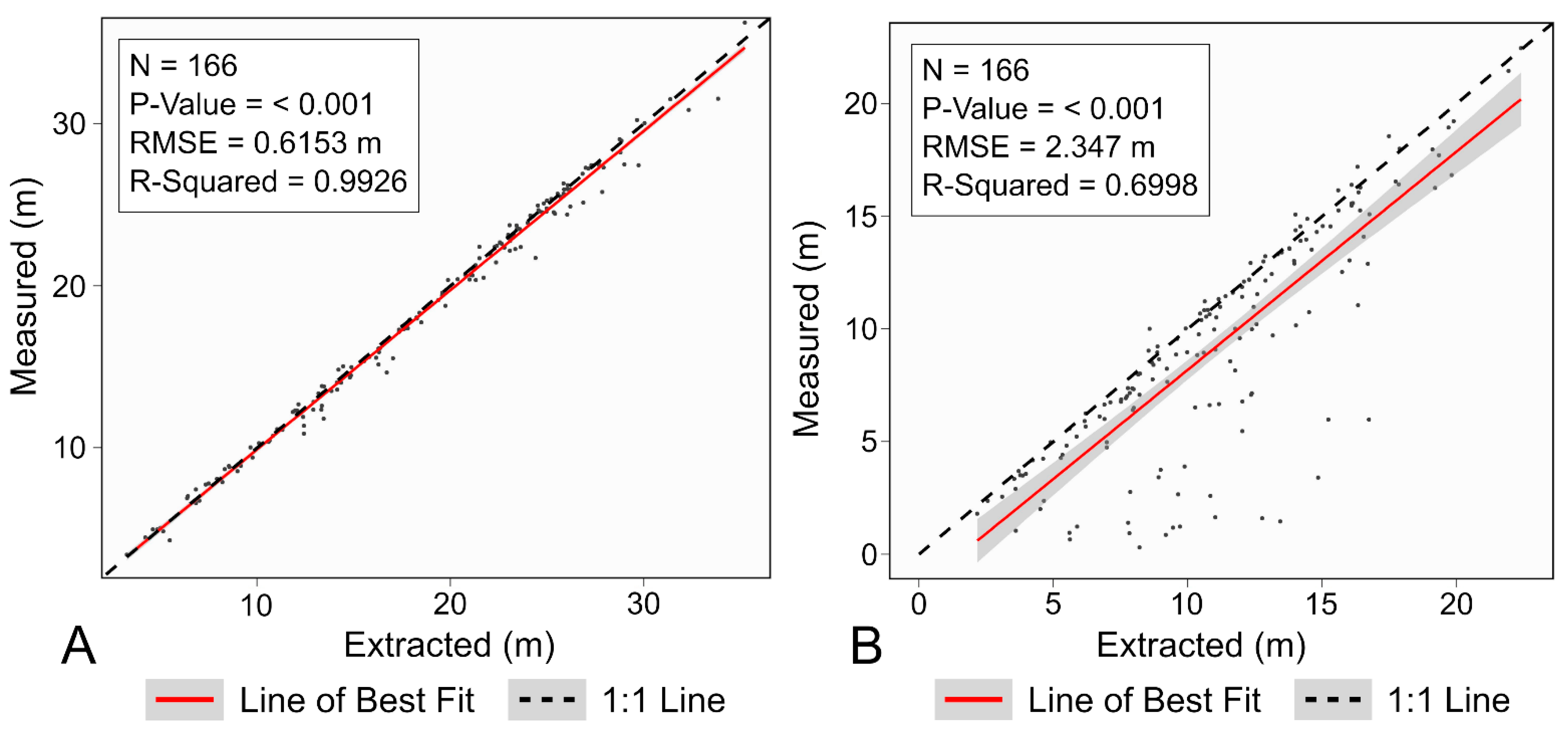
The vertical arrangement of the extracted and measured clusters was in relatively close agreement (Figure 6). The extracted upper boundaries corresponded well to the measured upper boundaries. This correspondence is exhibited by an R-squared value of 0.9926, low variance (0.6153 m), and a line of best fit that closely matches the 1:1 line. The extracted lower boundaries did not predict the measured values as well, with a lower R-squared value (0.6998) and higher variance (2.347 m). In many cases, the automated method substantially overpredicted the lower boundary of matched clusters, resulting in many points below the 1:1 line.
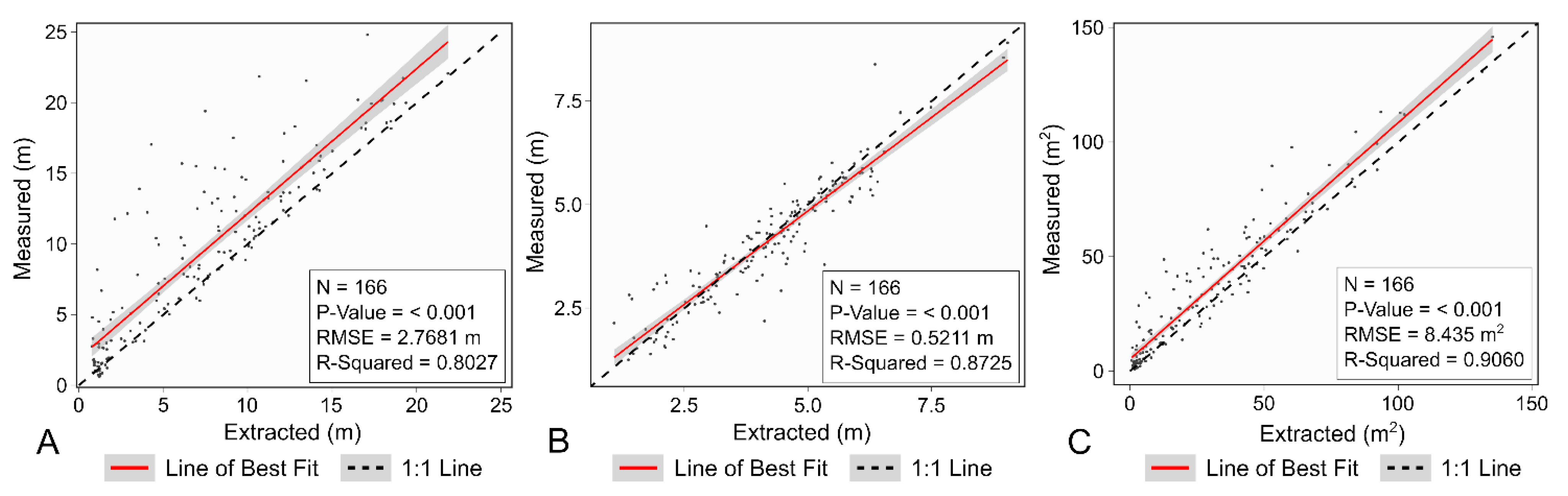
Figure 7 shows relatively strong agreement between the extracted and measured branch cluster dimensions. The extracted cluster diameters and volumes relate well to their manually measured counterparts, with respective R-squared values of 0.8725 and 0.9060. While still exhibiting a relatively strong relationship, the extracted vertical length of each cluster did not predict the measured values as well as the other two metrics. This deviation mirrors the relationship exhibited between the lower boundary of extracted and measured clusters shown in Figure 6. In this instance, the automated method often underpredicts the vertical length of each cluster.

3.3. Tree-Level Validation
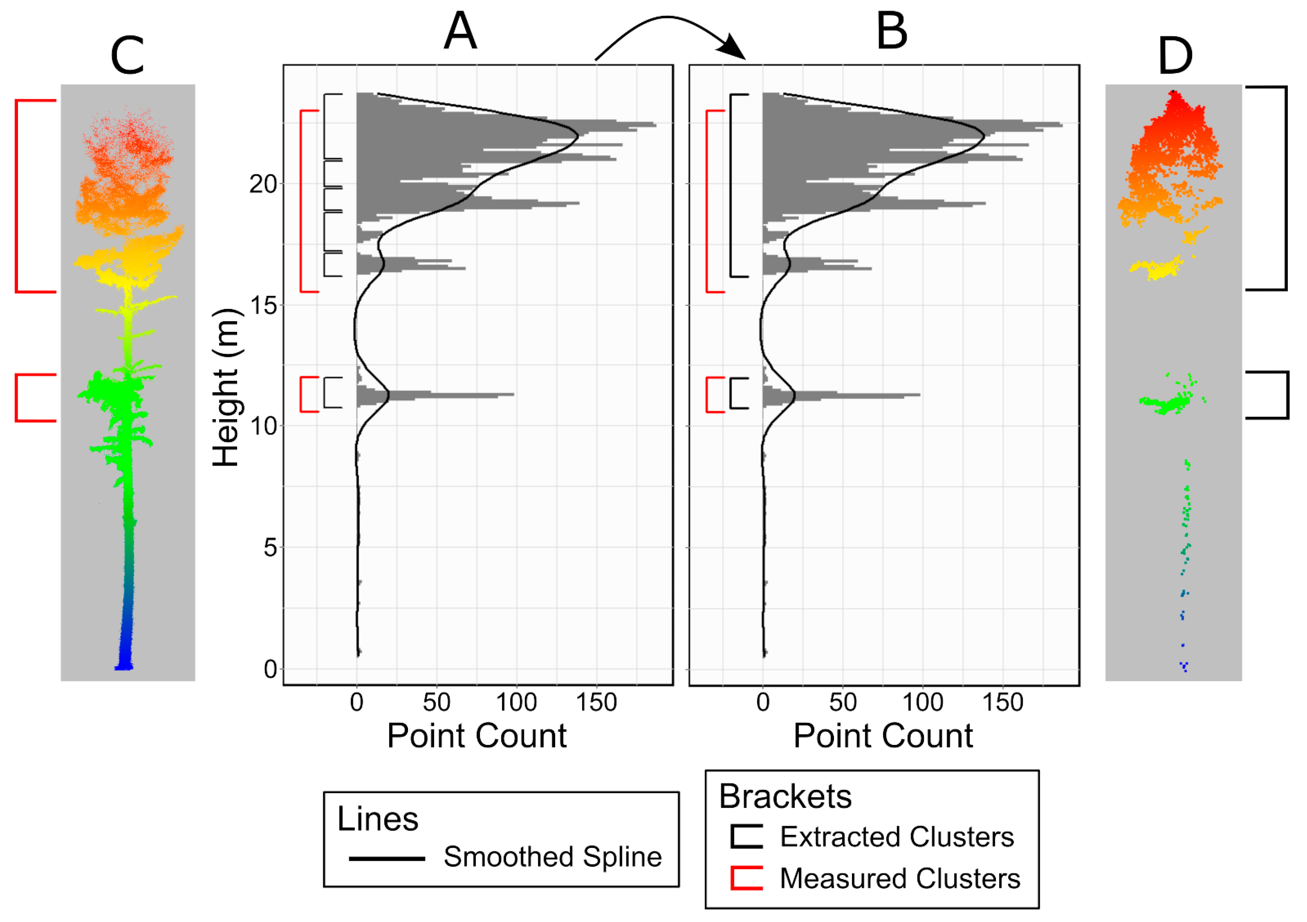
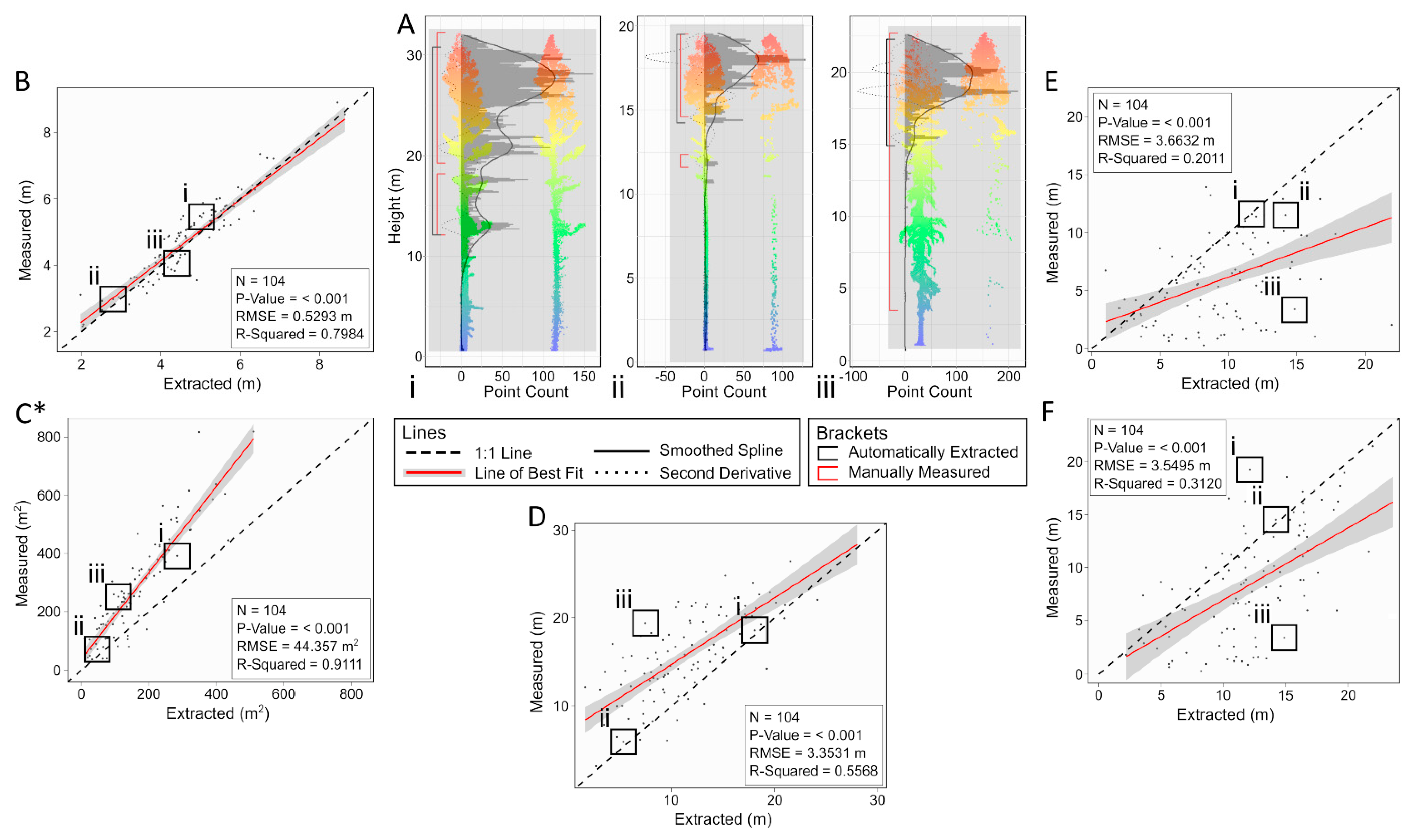
The focal point of Figure 8 illustrates three pairs of MLS and RPAS LiDAR point clouds. Each pair represents a different tree (i, ii, iii) that was used within this study. The histograms, splines, second derivative lines, and extracted clusters shown here were calculated from the distribution of the RPAS LiDAR point height. Comparing these features with the MLS point clouds and the manually measured clusters highlights the level of detail provided by these two types of point clouds. The subpanels show relationships between the extracted and measured values for the tree-level metrics, highlighting the values for each of the three example trees.
The agreement between measured and extracted attributes were more variable at the tree-level than at the cluster-level. Most extracted metrics either under- or overpredict their respective validation metrics. The strongest match was observed for crown width, which had a line of best fit that closely matched the 1:1 line. The extracted and measured total live branch volumes corresponded strongly (R-squared of 0.9111), although a consistent underprediction can be observed. The remaining three metrics had moderate to weak relationships. Of these, the live crown length exhibited the strongest relationship. This metric had an R-squared value of 0.5568, although it tended to underpredict the measured values, especially for the smaller trees. Neither the height of the lowest live branch nor the live crown base height was accurately predicted using the automated method. For both these metrics, the automated method consistently assumed a higher height than was manually measured.
Among the three examples of the MLS and RPAS LiDAR point clouds, differences were greatest in lower portions of the crown, especially for tree iii. Tracing the extracted and measured values for tree iii across each of the five scatter plots shows how differences in lower crown point counts and densities impacted the results of this study. The automated method overpredicted the height of the lowest live branch and the live crown base height. This was primarily due to the relative absence of these lower crown points from the RPAS LiDAR point cloud. These overpredictions also corresponded to an underprediction for the vertical crown length. Tree ii had nearly all the same features present in both point clouds, but the automated method did not detect the lowest manually measured live branch. This resulted in a slight overprediction of the lowest live branch height. This cluster was present in the RPAS LiDAR point cloud, but not in great enough detail to be extracted by the automated method. Tree i also had nearly all the same branch clusters present in both point clouds, but the automated method was unable to detect the same gaps as the validation dataset. This resulted in a large underprediction of live crown base height, something that was not indicative of the general trend associated with live crown base height relationship.

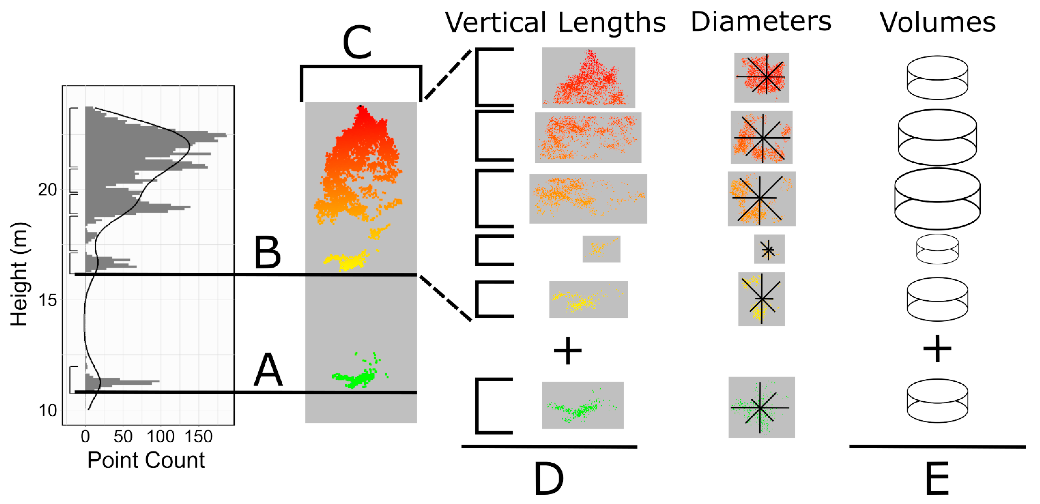
3.4. Summary of Extracted Tree-Level Data

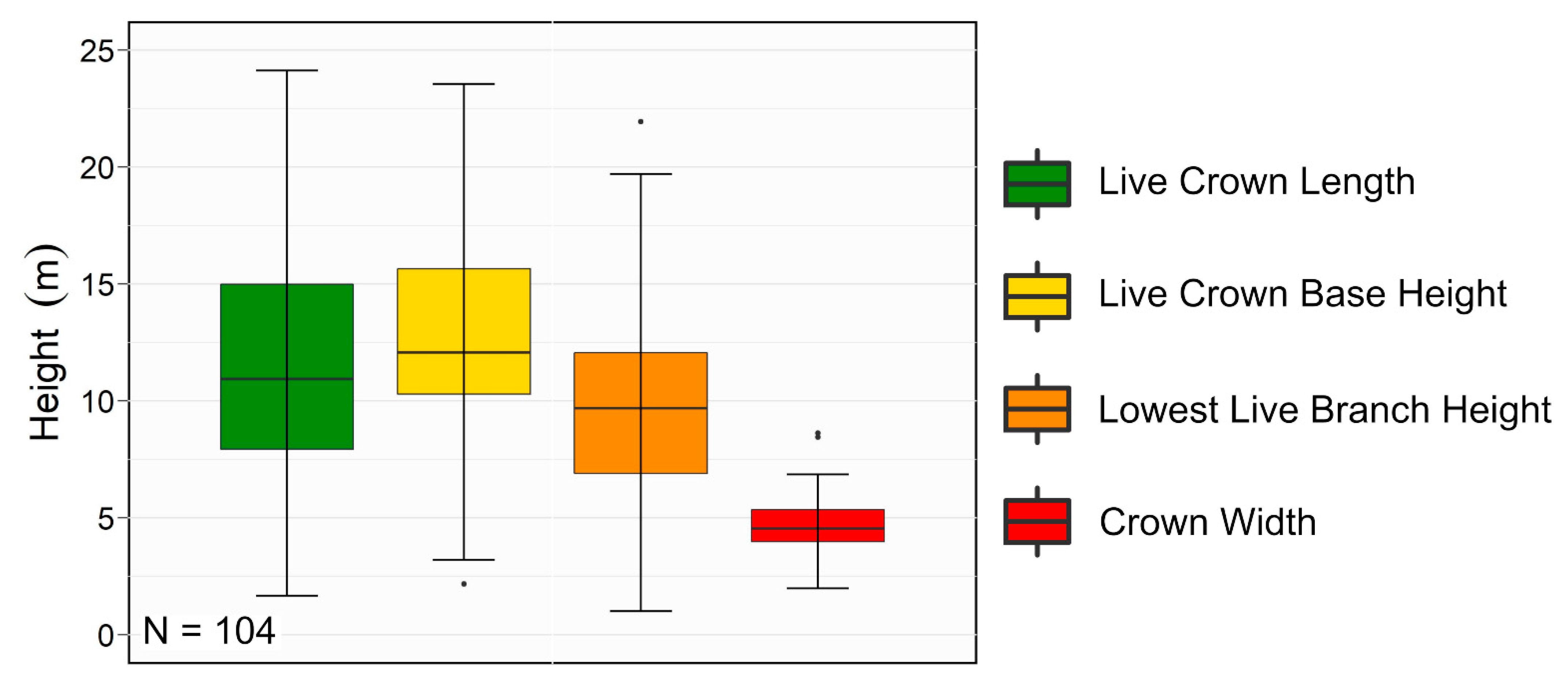
Figure 9 shows box and whisker plots for four tree-level metrics extracted from 104 trees using the automated method developed for this study. The values for live crown length had the largest range, followed by live crown base height and the height of the lowest live branch. Crown width values were most consistent, showing relatively little deviation from the median value of ~4.5 m. The overall and interquartile ranges of these four metrics were indicative of the variability observed in the sampled trees. This same variability was observed in the three example trees shown in Figure 8. Each tree shown had variable amounts and arrangement of living fuel, while having relatively similar crown widths.

4. Discussion

This study evaluated the ability of RPAS LiDAR point clouds to characterize the vertical arrangement and volume of crown fuels within individual trees. The new method extracted and quantified branch structures that contained live fuel and compared cluster and tree-level measurements to manual measurements collected from MLS point clouds. The differences between the extracted and measured metrics revealed important strengths and weaknesses of both the method and the utility of both types of point clouds.

4.1. Cluster-Level Fuels

The cluster-level analysis supports the utility of RPAS LiDAR to characterize fine-scale, within-tree geometry at a level of detail similar to TLS or MLS point clouds. This is particularly true for the more dominant portions of the tree crowns. Over 96% of all automatically extracted live branch clusters were successfully matched to manually measured branch clusters, which represented a similarly large proportion of all extracted volume. While a smaller proportion of manually measured branch clusters were matched to extracted clusters (~79%), the unmatched clusters represented less than 2% of the measured volume.
Comparing the vertical arrangement and dimensions of matched clusters revealed strong correspondences between the two datasets. The vertical arrangement of each cluster can be described by the lower and upper boundaries, both of which were predicted well, albeit not as strongly for the lower boundaries. The overprediction of these lower boundaries was mirrored by a general underprediction of the measured vertical length of each cluster. The measured diameter of each cluster was also predicted quite well by the automated method and did so without an under or overprediction. The vertical length and diameter of each cluster were used to calculate a simple cylindrical volume for each cluster. Comparing the measured and extracted volumes revealed a strong correspondence. While these results only considered matched clusters, the favorable trends support the use of this method and data for the evaluation of within-tree geometry.

4.2. Tree-Level Fuels

The aggregation of cluster-level information at the tree-level revealed more nuanced information about how RPAS LiDAR and MLS point clouds compare. This aggregation also shows the degree to which this method can extract tree-level information. While the automated method presented here is not infallible, many of the shortcomings presented in the tree-level results can be attributed to inherent differences between MLS and RPAS LiDAR point clouds. The overall differences in the quality of each point cloud were evident at the onset of this study by the much higher density of MLS point clouds. There were additional differences related to where each point cloud was collected. Due to the ground-based system, the majority of the MLS points were located beneath the base of the live crown, whereas the majority of the RPAS LiDAR points were located above this level. These differences resulted in overpredictions of live crown base height and the height of the lowest live branches. These inaccuracies are also mirrored by an underprediction of crown length. The reduced level of detail in the lower crown can also be observed in nearly every point cloud shown above.
Of the tree-level metrics evaluated in this study, the strongest relationships were observed for crown width and total live branch volume. Both these values can be reliably extracted from dominant portions of the crown that tend to be readily visible from airborne platforms. While extracted total live branch volume exhibited a very strong relationship with the measured values, it did so with a strong overprediction. This overprediction is partially due to undetected live fuels in the lower crown, but more so due to instances where multiple extracted clusters were contained within a single measured cluster. The measured clusters would have only been represented by a single cylinder with a constant diameter. The extracted method would instead represent these same clusters with multiple smaller cylinders, only one of which would have the same diameter as the manually measured cluster. This difference in volumetric calculations resulted in large differences between the extracted and measured values.
Live crown base height was calculated in a way that is similar to existing field-based methods [8]. While frequently applied, these methods can ignore fuel beneath the base of the primary crown, depending on the amount of vertical separation between fuel layers. In theory, accurate measures of live crown base height could be used in conjunction with crown width to calculate a simplistic crown volume. However, these types of methods would likely underrepresent the amount of fuel in lower portions of trees. Nearly 40% of the manually measured trees had living fuel between the ground and the base of the live crown. Of these trees, the average volume of fuel in this zone represented almost 12% of the total tree volume, and in some cases, over half the total volume.
This method was able to accurately characterize the locations and dimensions of the majority of live branch clusters, but not as reliably for lower clusters. This shortcoming is primarily a result of differences in the analyzed and reference data. Ground-based LiDAR is able to capture small features beneath the primary crown much more reliably than airborne LiDAR. Furthermore, the extremely low commission errors speak to the ability of the method to detect features that are present within a given point cloud. Therefore, the accurate extraction of these lower crown features is dependent on the quality and density of the provided point cloud. Overall, this work demonstrates a method that can reliably predict the amount and locations of large proportions of the total crown fuel present within a given tree.

4.3. Links to Past Research

The results of this study support and refine earlier work regarding the strengths and weaknesses of remotely derived airborne and ground-based point clouds. It has been shown that low density LiDAR point clouds collected from conventional aircraft can be used to successfully characterize stand-level overstory fuels [16,17,18]. Although depending on point density and canopy cover, fuels below the primary crown are unable to be characterized to the same degree as ground-based point clouds [38]. The results demonstrated here potentially extend this relationship to RPAS LiDAR point clouds, regardless of their high point density compared to conventional LiDAR point clouds. While not quantitatively evaluated in this study, tree segmented from RPAS LiDAR point clouds had more complete reconstructions in instances where the surrounding canopy cover was low. Similar observations were made for trees that had simpler crown structures.
The definition of crown base height that was used in this study allowed gaps of up to 25 cm to exist within a “continuous” crown. Similar methods as were presented here can be used to extract a flexible measurement of live crown base height with variable levels of gaps between live branches. This kind of measurement could represent a potentially significant outcome of this research. Crown base height definitions that rely on fixed gap thresholds assume that fire can only spread between crown layers separated by vertical gaps lower than the threshold. In this way, these definitions assume a fixed flame length, something that has long been understood to be variable depending on fuel and weather conditions [39]. This research also supports earlier work [9] by providing tools that can be used to model crown volume using non-uniform distributions of crown fuel. While contributing to this type of research, it is important to note that this work does not incorporate any information on the weights of available fuel, instead focusing on quantifying the three-dimensional volumes of portions of trees that contain available fuel.

4.4. Limitations and Future Work

The greatest limitation of this new method is the inability to extract lower crown fuels such as live crown base height and the height of the lowest live branches. While these missed branches were likely small in volume, their absence would likely result in an underprediction of true fire behaviour. This is especially true in cases where they are in close vertical proximity to other live crown fuels, thereby representing ladder fuels. Applying these methods directly to point clouds that have higher point densities beneath the primary crown would likely improve the characterization of these lower crown fuels. Typically, these types of point clouds are collected at the plot-level, thereby limiting their spatial scale. Recent advancements in RPAS and MLS systems have allowed the two to be combined for beneath canopy flights [40], allowing MLS data to be collected across larger spatial scales.
The method developed in this study was only applied to trees that were well segmented, which were primarily composed of the more dominant, overstory trees. These segmentation results are supported by previous research, which has shown that perfectly segmenting non-dominant, subcanopy trees can be exceedingly difficult, if not impossible [27,28,29]. The removal of poorly segmented trees was necessary to ensure the quality of the extracted trees, but drastically reduced the number of analyzed trees. This type of manual removal of trees results in the methods presented here being unable to be applied across most forest stands. Therefore, improvements in the quality and reliability of automatic tree segmentation algorithms should be seen as a prerequisite to the broader applications of individual-tree-based work. A collaborative approach between multi-disciplinary researchers is likely required. The authors support the creation of an open dataset of point clouds that could be used to further develop of these algorithms. Ideally, such a dataset would include various types of segmented and non-segmented point clouds collected from a range of forest types.
It is important to note that the volumes reported in this study do not necessarily represent the true volume of each live branch cluster or individual tree. This work instead relied on automated methods and manual measurements that assumed a tree was composed of a series of cylinders of various vertical lengths and diameters. This was done primarily to allow for manual measurements to be used for validation without having to destructively sample trees. While these methods are an improvement to existing field-based method, they likely overestimate the true volume of each live branch cluster and therefore the total volume. In reality, these volumes vary depending on how detailed the shapes are that are used to measure them, with finer detailed shapes providing more accurate volume estimates. Therefore, we suggest future research follow similar methods but use an approach that calculates the three-dimensional volume of each cluster using detailed alpha shapes. This type of work could then be used to improve conventional fire behaviour and fuel models by pairing these methods with destructive sampling-based techniques. Such methods could be used to develop novel, fine-scale allometric models that could predict the weight of the fuel within each cluster. This could be used along with the cluster volumes to extract inner-tree crown bulk density measurements. These fine-scale measurements could then be used to provide more accurate stand-level canopy bulk density measurements. Additionally, the fine-scale of the metrics extracted by these methods suggest that they could be used to build and further develop next-generation fire behaviour models, such as those described in [41].

5. Conclusions

This research demonstrates a new method that can be used to automatically detect and measure the arrangement and amount of live crown fuels within individual trees. This work shows that RPAS LiDAR point clouds can be used to characterize the majority of within-tree crown fuels at similar accuracies as MLS point clouds. Nearly 80% of all measured crown fuel clusters were matched to an extracted cluster. Metrics extracted from these matched clusters were in close agreement. Vertical arrangements and dimensions had R-squared values ranging from ~0.70 to ~0.99. The agreement between measured and extracted tree-level metrics were much more variable. The strongest relationships were observed for total volume and crown width, each of which had R-squared values over ~0.80. Metrics that included lower crown features had much lower levels of agreement, with R-squared values ranging from ~0.56 to ~0.20. Overall, this work supports the value that these types of methods and data can have for fuel and wildfire management. However, important limitations of the developed methodology and RPAS LiDAR point clouds, specifically, an inability to extract the lowest portions of crown fuels, should be considered. Future work should continue to improve the quality of individual tree segmentations, which would allow these types of studies to be implemented over larger scales. These methods also have potential to be paired with destructive sampling-based methodologies. Such a pairing could better parametrize the cluster and total crown volumes and potentially incorporate the weights of combustible fuels.

Author Contributions

Conceptualization, J.A., N.C.C., L.D.D. and A.P.; methodology, J.A. and N.C.C.; formal analysis, J.A.; investigation, J.A.; writing—original draft preparation, J.A.; writing—review and editing, J.A., N.C.C., L.D.D. and A.P.; visualization, J.A.; supervision, N.C.C., L.D.D. and A.P.; funding acquisition, J.A., N.C.C. and L.D.D. All authors have read and agreed to the published version of the manuscript.

Funding

This research was funded by FYBR Solutions Inc., Natural Sciences and Engineering Research Council of Canada (NSERC) grant CRDPJ 507166-16, and a donation from an anonymous foundation.

Data Availability Statement

The data presented in this study are available on request from the corresponding author.

Acknowledgments

The authors would like to thank the support of the IRSS lab as a whole, especially the following people who assisted with the collection of the remotely sensed data: Mike Wilcox, Tristan Goodbody, Felix Poulin, Lukas Jarron, Chris Mulverhill, and Nicholas Leach, as well as Daisy Qin Rui Zhao, who collected the validation data.

Conflicts of Interest

The authors declare no conflict of interest.

References

  1. Burton, P.J.; Parisien, M.A.; Hicke, J.A.; Hall, R.J.; Freeburn, J.T. Large fires as agents of ecological diversity in the North American boreal forest. Int. J. Wildl. Fire 2008, 17, 754–767. [Google Scholar] [CrossRef]
  2. Prichard, S.J.; Stevens-Rumann, C.S.; Hessburg, P.F. Tamm Review: Shifting global fire regimes: Lessons from reburns and research needs. For. Ecol. Manag. 2017, 396, 217–233. [Google Scholar] [CrossRef]
  3. Stephens, S.L.; Burrows, N.; Buyantuyev, A.; Gray, R.W.; Keane, R.E.; Kubian, R.; Liu, S.; Seijo, F.; Shu, L.; Tolhurst, K.G.; et al. Temperate and boreal forest mega-fires: Characteristics and challenges. Front. Ecol. Environ. 2014, 12, 115–122. [Google Scholar] [CrossRef] [Green Version]
  4. Thomas, D.; Butry, D.; Gilbert, S.; Webb, D.; Fung, J. The Costs and Losses of Wildfires: A Literature Review. NIST Spec. Publ. 2017, 1215, 72. [Google Scholar] [CrossRef]
  5. Rebain, S.A.; Reinhardt, E.D.; Crookston, N.L.; Beukeme, S.J.; Kurz, W.A.; Greenough, J.A.; Robinson, D.C.E.; Lutes, D.C. The Fire and Fuels Extension to the Forest Vegetation Simulator; United States Department of Agriculture, Forest Service, Rocky Mountain Research Station: Ogden, UT, USA, 2015. [Google Scholar]
  6. Cruz, M.G.; Alexander, M.E.; Wakimoto, R.H. Assessing canopy fuel stratum characteristics in crown fire prone fuel types of western North America. Int. J. Wildl. Fire 2003, 12, 39–50. [Google Scholar] [CrossRef] [Green Version]
  7. Reinhardt, E.; Lutes, D.; Scott, J. FuelCalc: A Method for Estimating Fuel Characteristics. In Fuels Management—How to Measure Success: Conference Proceedings; U.S. Department of Agriculture, Forest Service, Rocky Mountain Research Station: Fort Collins, CO, USA, 2006; Volume 41, pp. 273–282. [Google Scholar]
  8. Smith, F.W.; Keyser, T.; Shepperd, W. Estimating canopy fuels and their impact on potential fire behavior for ponderosa pine in the Black Hills, South Dakota; JFSP Research Project Reports; 2009; Volume 138, Available online: http://digitalcommons.unl.edu/jfspresearch/138 (accessed on 15 November 2021).
  9. Ex, S.A.; Smith, F.W.; Keyser, T.L.; Rebain, S.A. Estimating Canopy Bulk Density and Canopy Base Height for Interior Western US Conifer Stands. For. Sci. 2016, 62, 690–697. [Google Scholar] [CrossRef]
  10. Reinhardt, E.; Scott, J.; Gray, K.; Keane, R. Estimating canopy fuel characteristics in five conifer stands in the western United States using tree and stand measurements. Can. J. For. Res. 2006, 36, 2803–2814. [Google Scholar] [CrossRef]
  11. Keyser, T.; Smith, F.W. Influence of crown biomass estimators and distribution on canopy fuel characteristics in ponderosa pine stands of the Black Hills. For. Sci. 2010, 56, 156–165. [Google Scholar]
  12. Scott, J.H.; Reinhardt, E.D. Assessing crown fire potential by linking models of surface and crown fire behavior; U.S. Department of Agriculture, Forest Service, Rocky Mountain Research Station: Fort Collins, CO, USA, 2001; pp. 1–62. [Google Scholar] [CrossRef] [Green Version]
  13. Cole, D.M. Models for Describing Vertical Crown Development of Lodgepole Pine Stands; U.S. Department of Agriculture, Forest Service, Intermountain Forest and Range Experiment Station: Ogden, UT, USA, 1982; p. 10. Available online: https://catalog.hathitrust.org/Record/007413639 (accessed on 15 November 2021).
  14. Ottmar, R.D.; Vihnanek, R.E.; Wright, C.S. Stereo Photo Series for Quantifying Natural Fuels: Hardwood, Pitch Pine, and Red Spruce Volume I: Mixed-conifer with mortality, western juniper, sagebrush, and grassland types in the interior Pacific Northwest. 1998, 830, 73.
  15. Schomaker, M.E.; Zarnoch, S.J.; Bechtold, W.A.; Latelle, D.J.; Burkman, W.G.; Cox, S.M. Crown-Condition Classification: A Guide to Data Collection and Analysis; US Department of Agriculture, Forest Service, Southern Research Station: Asheville, NC, USA, 2007; p. 92. [Google Scholar] [CrossRef]
  16. Andersen, H.E.; McGaughey, R.J.; Reutebuch, S.E. Estimating forest canopy fuel parameters using LIDAR data. Remote Sens. Environ. 2005, 94, 441–449. [Google Scholar] [CrossRef]
  17. Erdody, T.L.; Moskal, L.M. Fusion of LiDAR and imagery for estimating forest canopy fuels. Remote Sens. Environ. 2010, 114, 725–737. [Google Scholar] [CrossRef]
  18. González-Ferreiro, E.; Diéguez-Aranda, U.; Crecente-Campo, F.; Barreiro-Fernández, L.; Miranda, D.; Castedo-Dorado, F. Modelling canopy fuel variables for Pinus radiata D. Don in NW Spain with low-density LiDAR data. Int. J. Wildl. Fire 2014, 23, 350–362. [Google Scholar] [CrossRef]
  19. Pyorala, J.; Liang, X.; Vastaranta, M.; Saarinen, N.; Kankare, V.; Wang, Y.; Holopainen, M.; Hyyppa, J. Quantitative assessment of scots pine (Pinus Sylvestris L.) whorl structure in a forest environment using terrestrial laser scanning. IEEE J. Sel. Top. Appl. Earth Obs. Remote Sens. 2018, 11, 3598–3607. [Google Scholar] [CrossRef] [Green Version]
  20. Lau, A.; Bentley, L.P.; Martius, C.; Shenkin, A.; Bartholomeus, H.; Raumonen, P.; Malhi, Y.; Jackson, T.; Herold, M. Quantifying branch architecture of tropical trees using terrestrial LiDAR and 3D modelling. Trees-Struct. Funct. 2018, 32, 1219–1231. [Google Scholar] [CrossRef] [Green Version]
  21. Hosoi, F.; Nakai, Y.; Omasa, K. 3-D voxel-based solid modeling of a broad-leaved tree for accurate volume estimation using portable scanning lidar. ISPRS J. Photogramm. Remote Sens. 2013, 82, 41–48. [Google Scholar] [CrossRef]
  22. Cabo, C.; Del Pozo, S.; Rodríguez-Gonzálvez, P.; Ordóñez, C.; González-Aguilera, D. Comparing terrestrial laser scanning (TLS) and wearable laser scanning (WLS) for individual tree modeling at plot level. Remote Sens. 2018, 10, 540. [Google Scholar] [CrossRef] [Green Version]
  23. Meidinger, D.V.; Pojar, J. Ecosystems of British Columbia; Special Report Series; Ministry of Forests: Victoria, BC, Canada, 1991; ISBN 0771889976. [Google Scholar]
  24. Leclerc, M.A.F.; Daniels, L.D.; Carroll, A.L. Managing Wildlife Habitat: Complex Interactions With Biotic and Abiotic Disturbances. Front. Ecol. Evol. 2021, 9, 613371. [Google Scholar] [CrossRef]
  25. Stal, C.; Verbeurgt, J.; De Sloover, L.; De Wulf, A. Assessment of handheld mobile terrestrial laser scanning for estimating tree parameters. J. For. Res. 2020. [Google Scholar] [CrossRef]
  26. Besl, P.J.; McKay, N.D. A method for registration of 3-D shapes. IEEE Trans. Pattern Anal. Mach. Intell. 1992, 14, 239–256. [Google Scholar] [CrossRef]
  27. Li, W.; Guo, Q.; Jakubowski, M.K.; Kelly, M. A New Method for Segmenting Individual Trees from the Lidar Point Cloud. Photogramm. Eng. Remote Sens. 2012, 78, 75–84. [Google Scholar] [CrossRef] [Green Version]
  28. Yancho, J.M.M.; Coops, N.C.; Tompalski, P.; Goodbody, T.R.H.; Plowright, A. Fine-Scale Spatial and Spectral Clustering of UAV-Acquired Digital Aerial Photogrammetric (DAP) Point Clouds for Individual Tree Crown Detection and Segmentation. IEEE J. Sel. Top. Appl. Earth Obs. Remote Sens. 2019, 12, 4131–4148. [Google Scholar] [CrossRef]
  29. Jakubowski, M.K.; Li, W.; Guo, Q.; Kelly, M. Delineating individual trees from lidar data: A comparison of vector- and raster-based segmentation approaches. Remote Sens. 2013, 5, 4163–4186. [Google Scholar] [CrossRef] [Green Version]
  30. Edelsbrunner, H.; Mücke, E.P. Three-Dimensional Alpha Shapes. ACM Trans. Graph. 1994, 13, 43–72. [Google Scholar] [CrossRef]
  31. Luo, L.; Zhai, Q.; Su, Y.; Ma, Q.; Kelly, M.; Guo, Q. Simple method for direct crown base height estimation of individual conifer trees using airborne LiDAR data. Opt. Express 2018, 26, A562. [Google Scholar] [CrossRef]
  32. CloudCompare. Available online: http://www.danielgm.net/cc/ (accessed on 15 November 2021).
  33. Isenburg, M. LAStools—Efficient LiDAR Processing Software. Available online: https://rapidlasso.com/lastools/ (accessed on 15 November 2021).
  34. Roussel, J.R.; Auty, D.; Coops, N.C.; Tompalski, P.; Goodbody, T.R.H.; Meador, A.S.; Bourdon, J.F.; de Boissieu, F.; Achim, A. lidR: An R package for analysis of Airborne Laser Scanning (ALS) data. Remote Sens. Environ. 2020, 251, 112061. [Google Scholar] [CrossRef]
  35. Roussel, J.-R.; Auty, D. Airborne LiDAR Data Manipulation and Visualization for Forestry Applications 2021. Available online: https://cran.r-project.org/package=lidR (accessed on 15 November 2021).
  36. Silva, C.A.; Crookston, N.L.; Hudak, A.T.; Vierling, L.A.; Klauberg, C.; Cardil, A.; Hamamura, C. rLiDAR: LiDAR Data Processing and Visualization 2021. Available online: https://cran.r-project.org/package=rLiDAR (accessed on 15 November 2021).
  37. Lafarge, T.; Pateiro-Lopez, B. alphashape3d: Implementation of the 3D Alpha-Shape for the Reconstruction of 3D Sets from a Point Cloud 2020. Available online: https://cran.r-project.org/package=alphashape3d (accessed on 15 November 2021).
  38. Calders, K.; Schenkels, T.; Bartholomeus, H.; Armston, J.; Verbesselt, J.; Herold, M. Monitoring spring phenology with high temporal resolution terrestrial LiDAR measurements. Agric. For. Meteorol. 2015, 203, 158–168. [Google Scholar] [CrossRef]
  39. Byram, G.M. Combustion of forest fuels. In Forest Fire: Control and Use; Davis, K.P., Ed.; McGraw-Hill: New York, NY, USA, 1959; pp. 61–89. [Google Scholar]
  40. Hyyppä, J.; Yu, X.; Hakala, T.; Kaartinen, H.; Kukko, A.; Hyyti, H.; Muhojoki, J.; Hyyppä, E. Under-Canopy UAV Laser Scanning Providing Canopy Height and Stem Volume Accurately. Forests 2021, 12, 856. [Google Scholar] [CrossRef]
  41. Mell, W.E.; Manzello, S.L.; Maranghides, A.; Butry, D.; Rehm, R.G. The wildland—urban interface fire problem—current approaches and research needs. Int. J. Wildl. Fire 2010, 19, 238–251. [Google Scholar] [CrossRef]
Figure 1. Location of the 17 plots in the Alex Fraser Research Forest (AFRF) near Williams Lake, Canada.
Remotesensing 13 04598 g001
Figure 2. Examples of the two types of point clouds from (A) mobile laser scanning (MLS) and (B) remotely piloted aerial systems (RPAS) LiDAR.
Remotesensing 13 04598 g002
Figure 3. An overview of the live branch cluster extraction method. (A) Originally segmented RPAS LiDAR point cloud; (B) thinned RPAS LiDAR point cloud; (C) histogram, spline, and derivative extractions; (D) initial cluster extraction; (E) removal of small clusters.
Remotesensing 13 04598 g003
Figure 4. An overview of the live branch cluster and total tree metric extraction. (A) Height of the lowest live branch cluster; (B) live crown base height; (C) crown width; (D) total crown length; (E) total live branch volume.
Remotesensing 13 04598 g004
Figure 5. Examples of manually measured live branch clusters compared to extracted clusters before and after cluster aggregation. (A) Histogram showing validation data compared to automatically extracted live branch clusters; (B) histogram showing validation data compared to extracted live branch clusters following their aggregation; (C) MLS point cloud with measured clusters; (D) thinned RPAS LiDAR point cloud with aggregated extracted clusters.
Remotesensing 13 04598 g005
Figure 6. Agreement between measured and extracted (A) upper and (B) lower boundaries of live branch clusters. In each panel, the line of best fit is displayed in red and the 1:1 line is shown as the dashed black line.
Remotesensing 13 04598 g006
Figure 7. Agreement between measured and extracted (A) vertical length, (B) diameters, and (C) volume of live branch clusters. In each panel, the line of best fit is displayed in red, and the 1:1 line is shown as the dashed black line.
Remotesensing 13 04598 g007
Figure 8. Tree-level point clouds and agreement between extracted and measured values for five metrics. (A) Point clouds (left—MLS, right—RPAS LiDAR), histograms, and merged live branch clusters for three example trees (i, ii, iii). Agreement between measured and extracted (B) crown width; (C*) total live branch volume (the points of 2 large trees were removed for display purposes); (D) live crown length; (E) lowest live branch height; (F) live crown base height.
Remotesensing 13 04598 g008
Figure 9. Box and whisker plot displaying extracted data for four crown measurements. Boxes represent the interquartile range and median values; whiskers represent the smallest and largest values within one and a half times the first and third quartiles; and points represent outliers.
Remotesensing 13 04598 g009
Table 1. Differences between the amount of extracted, measured, true positive, false positive, and false negative clusters. Statistics related to the heights and dimensions of each type of cluster and cluster matching results are also shown.
Type of ClusterCount (#)Mean Height (m)Mean Diameter (m)Mean Vertical Length (m)Mean Volume (m2)Total Volume (m2)
Extracted82516.113.971.4621.8418,020.53
Measured21012.613.717.87147.1330,897.07
True Positive79716.343.981.4621.7717,429.73
False Positive289.643.051.3321.10590.80
False Negative447.492.001.717.95349.57
Overall accuracy—91.72%Commission error—3.22%Omission error—5.06%
Publisher’s Note: MDPI stays neutral with regard to jurisdictional claims in published maps and institutional affiliations.

