Classification of Mediterranean Shrub Species from UAV Point Clouds

Abstract

Modelling fire behaviour in forest fires is based on meteorological, topographical, and vegetation data, including species’ type. To accurately parameterise these models, an inventory of the area of analysis with the maximum spatial and temporal resolution is required. This study investigated the use of UAV-based digital aerial photogrammetry (UAV-DAP) point clouds to classify tree and shrub species in Mediterranean forests, and this information is key for the correct generation of wildfire models. In July 2020, two test sites located in the Natural Park of Sierra Calderona (eastern Spain) were analysed, registering 1036 vegetation individuals as reference data, corresponding to 11 shrub and one tree species. Meanwhile, photogrammetric flights were carried out over the test sites, using a UAV DJI Inspire 2 equipped with a Micasense RedEdge multispectral camera. Geometrical, spectral, and neighbour-based features were obtained from the resulting point cloud generated. Using these features, points belonging to tree and shrub species were classified using several machine learning methods, i.e., Decision Trees, Extra Trees, Gradient Boosting, Random Forest, and MultiLayer Perceptron. The best results were obtained using Gradient Boosting, with a mean cross-validation accuracy of 81.7% and 91.5% for test sites 1 and 2, respectively. Once the best classifier was selected, classified points were clustered based on their geometry and tested with evaluation data, and overall accuracies of 81.9% and 96.4% were obtained for test sites 1 and 2, respectively. Results showed that the use of UAV-DAP allows the classification of Mediterranean tree and shrub species. This technique opens a wide range of possibilities, including the identification of species as a first step for further extraction of structure and fuel variables as input for wildfire behaviour models.

1. Introduction

Wildfires are the main cause of forest ecosystem disturbance in the Mediterranean basin, modifying the vegetation, fauna, soil, and affecting hydrological and geomorphological processes [1,2]. Although wildfires can have a natural origin, playing an important role in ecological cycles [3], their behaviour is being affected in the Mediterranean basin by anthropogenic activity [4,5,6,7]. Humans are modifying land use and climate causing an increase in wildfires and burned area, modifying their natural frequency and reducing their period of recurrence [8,9]. Since the mid-20th century, socioeconomic development has promoted rural–urban migration, causing the abandonment of the traditional land exploitation and increasing fuel loads, which imply a greater risk of igniting a forest fire [10]. Climate change models indicate that the Mediterranean basin will be one of the most affected globally by the rising of temperatures and reduction of precipitation, considering it as a climate change “hot spot” [4,11]. These factors together with the increasing of soil aridity will affect directly the fire regime [5], expecting the increase of wildfire frequency and burned areas [6].

The advancements in technology have enabled the improvement of wildfires knowledge through computational fire modelling [12,13,14]. Wildfire models simulate the behaviour of the fire, being a key approach to understanding the complex relationships between fire occurrence, fire drivers, and potential impacts. These models provide relevant information in the different phases of wildfires: prevention, suppression, and recovery [12]. New physics-based fire behaviour models use physical and empirical fire models coupled to computational fluid dynamic models to parametrise the interaction between the chemical combustion processes and the surrounding atmosphere, terrain, and vegetation [14,15,16]. In order to simulate these interactions, fire models such as FIRETEC [17] or the Wildfire Dynamics Simulator (WFDS) [15] work with millimetre spatial scales [13]. These models need a very fine resolution of terrestrial inputs to correctly perform the physical parameterisation of local-scale forest characteristics [14,16]. In this regard, the most important terrestrial variable when studying wildland fuels is the bulk density (BD) because it affects the fire spread and intensity [18,19]. BD is defined as the mass of the fuel component material by volume unit (kg·m⁻³) and represents the degree of fuel packing [18]. BD estimation is particularly complex as it is normally obtained from species-specific allometric equations, relating the dimensions of the plant and its dry weight [20,21]. These equations can be calculated at different levels of vegetation detail, from species groupings to individual divisions [21]. In this sense, the level of detail of the new generation of wildfire models makes it necessary to classify the area studied by species and individuals. This information allows for obtaining features such as BD with high accuracy and resolution.

The level of detail required to run the new wildfire models has highlighted the need to study not only the tree layer but also the shrub layer. In Mediterranean forest ecosystems, shrubs are an important component of surface fuels [21]. Shrubs have a high rate of energy exchange, being particularly relevant as an igniter and spreader of fires [22]. One of the greatest dangers when analysing a potential forest fire is the existence of ladder fuels, such as shrubs, that provide continuity between the different vertical strata [23]. In areas prone to wildfire, creating a separation in vegetation by removing ladder fuels is an important task to avoid crown fires. This type of fire spreads rapidly through the upper layer, where the wind usually blows stronger than in the lower layer [23].

Over the last decades, advances in remote sensing have allowed the classification of plant species using different types of platforms and sensors [24]. Remote sensors have traditionally been carried on satellites, aircrafts, or balloons, but in recent years the use of unmanned aerial vehicles (UAVs) has changed this paradigm [25]. Compared to traditional platforms, UAVs have many advantages, such as the cost of acquisition, maintenance, and operation, which is significantly lower compared to other platforms [26]. UAVs allow easy modification of the flight plan, adapting to the spatial and temporal resolution required for each project. In this sense, the possibility of modifying the flight altitude allows adapting to different weather conditions, being able to fly below cloud cover [27]. The low flight altitude, compared to other platforms, allows UAVs to obtain finer spatial resolution [27]. One of the major advantages of UAVs is that they only need to be equipped with a consumer camera to obtain products such as point clouds, 3D objects, or orthophotos, applying structure from motion (SfM) algorithms [26,28,29]. Point clouds derived from UAV-based digital aerial photogrammetry (UAV-DAP) provide 3D information, useful for the detection of differences in vertical structure (i.e., plant height, plant patterns, and leaf distribution) [30,31,32]. UAV-DAP point clouds can contain, in addition to geometric information, spectral information extracted from the original pixel value [29]. The instrumentation cost of this technique is determined by the optical sensor used, starting from the simplest consumer cameras to the most advanced hyperspectral sensors. On the other hand, some disadvantages of UAVs are their reduced payload and their instability under windy conditions. However, their main disadvantage compared to other platforms is the limited flight range; therefore, their use is reduced to small-scale projects [33]. In this respect, the main disadvantage of the UAV-DAP technique is its lack of penetration into the tree canopy, reducing the information obtained from the forest structure [32].

Some studies have used UAV-DAP data for classification of vegetation with accurate results [27,28,33,34]. Nevalainen et al. [27] detected and classified four tree species in boreal forests using UAV-DAP point clouds and hyperspectral image mosaics and compared different techniques of machine learning (k-nearest neighbours, Random Forest, and MultiLayer Perceptron). Tuominen et al. [33] also used UAV-DAP point clouds and hyperspectral image mosaics together with k-nearest neighbours and Random Forest classifiers with a more ambitious goal: to classify 26 different tree species. In the same line, Camile Sothe et al. [28] similarly used UAV-DAP and hyperspectral data to classify 12 species in a subtropical forest in Brazil. What all these studies have in common is that they provide a map of the classified species as a result. In contrast, Mesas-Carrascosa et al. [34] proposed the classification of UAV-DAP point clouds obtained from RGB imagery to determine the points belonging to vineyards. These points were used to determine vine height. Once the classification of the point cloud is done, three-dimensional information can be derived (e.g., tree heights), enabling a further application of this 3D information (e.g., as fire models’ input). In this sense, the classification of the point cloud of a forest area would imply the possibility of extracting information of the vegetation structure. In addition, Mesas-Carrascosa et al. [34] performed a classification using only consumer cameras, far from the capabilities and costs of hyperspectral sensors. There are currently few articles describing the classification of vegetation types using UAV-DAP point clouds. In this regard, to our knowledge there is no study that attempted to classify shrub species in addition to tree species using UAV-DAP point clouds, which is particularly interesting due to their importance in wildfire modelling.

In this paper, we propose a methodology for the classification of UAV-DAP derived point clouds in tree and shrub species’ types, using multispectral data with low spectral resolution cameras. We evaluated the methods in two Mediterranean shrub-dominated forest areas and compared the performance of different classifiers.

2. Materials and Methods

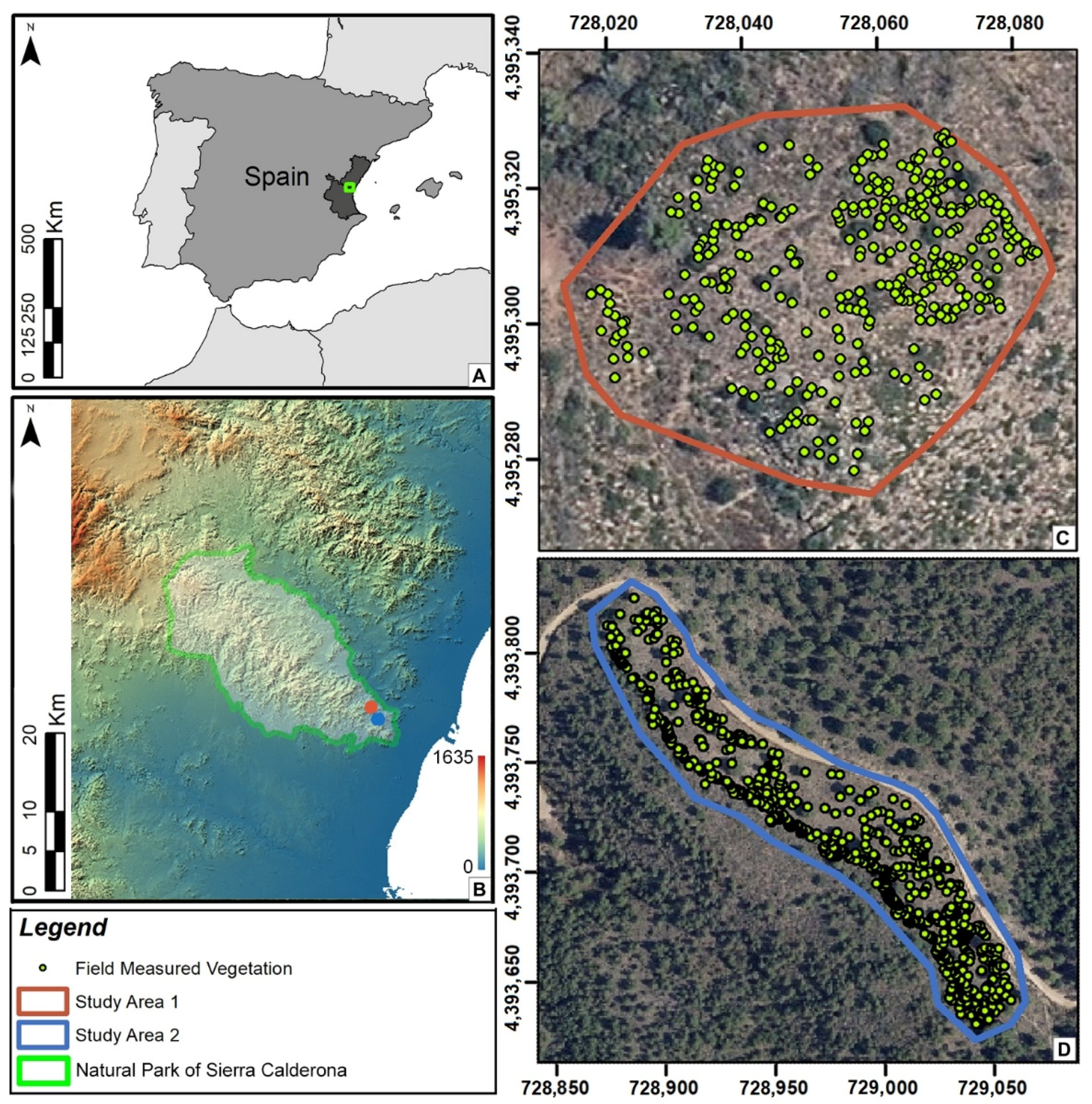
2.1. Study Sites

The study area is divided into two zones located in the Natural Park of Sierra Calderona, between the eastern Spain provinces of Valencia and Castellon (Figure 1). This Park is one of the most emblematic protected natural areas in the province of Valencia. The Sierra Calderona forms part of the last foothills of the Iberian System, being constituted by a NW-SE mountain range. Most of the area is below 1000 m above sea level and it is a typical example of a pre-coastal Valencian Mediterranean mountain range [29]. The climate is coastal Mediterranean with mild changes in temperature and a mean temperature of 16 °C. Rainfall in summer is low, contrasting with autumn and spring, where most of the annual rainfall is accumulated (450 mm) usually with torrential rains. The main species of the study areas and their description are listed in

Table 1. Summary of the species studied with their scientific and common names, description of their morphology, number of individuals analysed, number of training points selected in the point cloud to train the classifier, and study area where the species is located (value 1: study Area 1; value 2: study Area 2).

Scientific Name (Common Name)	Description of Shape and Colour	N. of Plants Measured	Number of Training Points	Study Area
Anthyllis cytisoides L. (Albaida)	Shrub with erect branches from the base. Greyish-whitish appearance, hairy in the younger parts.	18	1910	1
Chamaerops humilis L. (European fan palm)	Shrubby plant with a central stem, palmate fan, and very large green leaves.	73	5528	1
Cistus monspeliensis L. (Montpelier cistus)	Shrub with erect branches from the base. Linear-lanceolate dark green leaves.	90	5651	1
Genista scorpius (L.) DC. (Aulaga)	Greyish-green genistoid shrub, with a central stem and highly branched. Almost leafless (only in spring).	44	2627	1
Quercus coccifera L. (Kermes oak)	Dense shrub, very branched, covered with coriaceous and glabrous leaves, with shiny surface and intense green colour.	44	4187	1
Cistus albidus L. (Grey-leaf cistus)	Branched shrub with grey bark and glaucous-green ovate-lanceolate leaves. Whitish appearance.	66	1499	2
Juniperus oxycedrus L. (Cade juniper)	Shrub with a central trunk that branches a few centimetres above the ground. Needle-shaped leaves, very dense, and intense green colour.	81	7653	2
Pinus halepensis Mill. (Aleppo pine)	Tree with a rounded or flat-topped crown of slender, irregular horizontal, upturned branches. Intense green needles in fascicles.	33	3308	2
Rhamnus lycioides L. (Black hawthorn)	Shrub of medium or short stature, thorny, and highly branched from the base creating a thicket. The leaves are green grouped in fascicles.	83	3804	2
Salvia rosmarinus Schleid. (Rosemary)	Very branched shrub from the base. Branches densely covered with glossy green leaves on the upper surface and whitish on the lower.	245	32,596	2
Pistacia lentiscus L. (Mastic)	Branchy shrub that reaches the size of a small tree. Mature bark is greyish, but in the branches and young specimens it is reddish. Dark shiny leaves on the upper surface, somewhat lighter on the lower.	27; 102	2536; 4569	1; 2

.

The study site referred to as Area 1 encompasses 2889 m², where the existence of the current taxa derives from a forest fire that devastated 70 hectares of the Natural Park of Sierra Calderona in 2014. The ecological succession caused by the fire is defined by the presence of shrub species adapted to intense solar radiation, with an indifferent substrate and adapted to soils with a high degree of stoniness and poor in nutrients. The density of shrubs is very high and forms an almost continuous horizontal layer of vegetation, where the different species are mixed without exceeding 150 cm in height. There is no tree cover in the area. The study site referred to as Area 2 encompasses 11,455 m², where the vegetation is subject to preventive silvicultural treatments that have modified the fuel pattern. This area corresponds to a strip with a width between 20 and 30 m. It is characterised by scattered Pinus halepensis trees that are pruned to 2/3 of the tree height. The shrubs in this area are well formed and isolated.

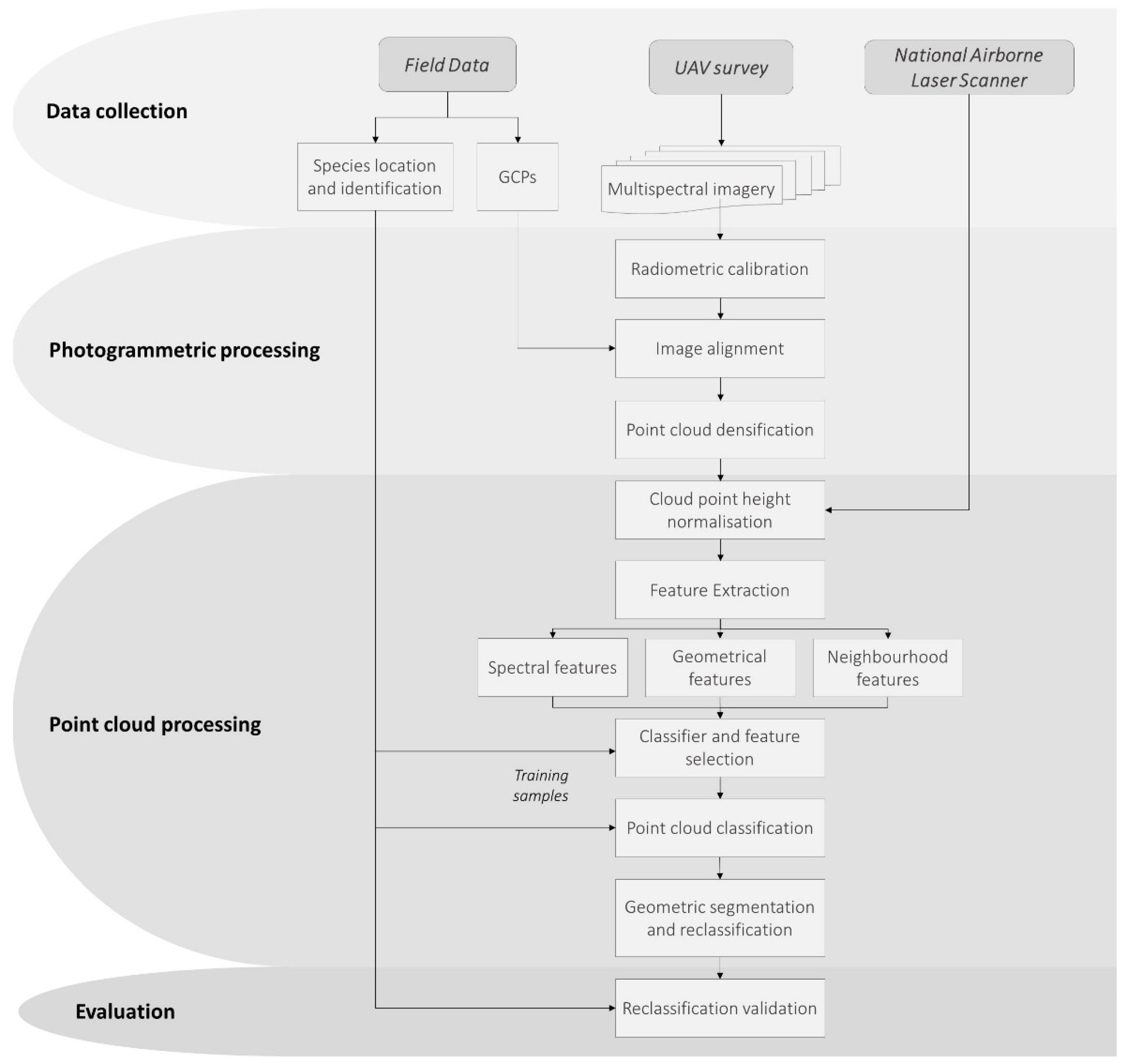
2.2. Overview of the Method

A general overview of the methodology is shown in Figure 2. Firstly, data collection was carried out from three different sources. Several multispectral flights were performed over the study areas and the positions of the Ground Control Points (GCPs) were collected by Global Navigation Satellite System (GNSS) and applying Real-Time Kinematic (RTK). This same technique was used to geolocate the position of the individuals studied; at the same time, the species of each individual were identified. ALS point clouds of the study area were obtained from the Spanish National Aerial Orthophotography Program (PNOA). In the second step we carried out the photogrammetric process to obtain the point clouds, where we performed a radiometric calibration of the multispectral images, aligned the images to reconstruct the flight scene, and densified the point cloud obtained during the alignment. In the next step we started the processing of the point clouds with the normalisation of the heights, where the bare ground points from the UAV-DAP and airborne laser scanning (ALS) point clouds were merged. Next, an extraction of spectral, geometric, and neighbourhood features from the point cloud was performed. Using the extracted features and training samples obtained from field data, a comparison of the following classifiers was performed: Decision Tree, Extra Trees, Gradient Boosting, Random Forest, and MultiLayer Perceptron. The method with the highest mean cross-validation scores was selected. Subsequently, a feature selection based on permutation feature importance and Pearson correlation was performed. Once the features were selected, the point cloud was classified using the selected classifier. In the last step of point cloud processing, we performed a segmentation of the point cloud based on its geometry, reclassifying it to regularise the classification. Finally, we validated the results obtained.

2.3. GNSS and UAV Data Collection

Fieldwork was carried out on 23–24 July 2020, performing an aerial multispectral data collection and a GNSS data collection campaign. UAV field work consisted of two flights (one per study area). Both flights were conducted close to solar noon to minimize shadowing, under sunny conditions, quite windless for the first flight and a light wind for the second flight. The campaign flights were conducted with a DJI Inspire 2 UAV, a quadcopter drone weighting 3.44 kg, with a maximum payload of 0.81 kg. Its four brushless motors are powered by two LiPo batteries of 4280 mAh, allowing for flights of up to 27 min, depending on the payload and meteorological conditions. The DJI Inspire 2 was equipped with a Micasense RedEdge multispectral camera (Micasense Inc., Seattle, WA, USA), with five spectral bands: blue (475-nm centre, 20-nm bandwidth), green (560 nm, 20-nm bandwidth), red (668 nm, 10-nm bandwidth), red edge (717 nm, 10-nm bandwidth), and near-infrared (840 nm, 40-nm bandwidth). The camera is composed of five sensors (4.8 × 3.6 mm) of 1.2 MP of resolution with focal length fixed at 5.5 mm, giving a sensor pixel size of 3.75 μm. The image format of this camera is 16-bit TIFF.

The flight of study Area 1 lasted 6 min, taking 1150 images (one per band) and covering an extension of 2.12 ha with a mean flying altitude of 49.2 m and a longitudinal and transverse overlap of 80%, whereas the flight over study Area 2 lasted 7 min, acquiring 1295 images over an extension of 2.79 ha with a mean flying altitude of 59.6 m and an overlap equal to the previous flight, 80%. In addition, several images of a calibration panel of known reflectance were taken before and after the flights for the radiometric calibration of the images.

During this campaign, the position and species of a total of 1036 individuals were collected, corresponding to the most representative shrub and tree species in both study areas (Table 1). In this work, the projection on the floor of the barycentre of each individual was taken by GNSS positioning. In addition, to increase the accuracy of georeferencing taken by UAV, during these works the centres of 12 GCPs were georeferenced (6 GCPs per study area). The GNSS survey equipment used during the field campaign was a Leica GPS1200 using a RTK technique with an accuracy of ±(10 mm + 1 ppm) and ±(20 mm + 1 ppm) in horizontal and vertical, respectively.

2.4. Photogrammetric Processing

All processes were carried out on a Windows 64-bit system, with the following specifications: RAM 32 GB, CPU IntelI CITM) i7-8700 CPU @ 3.20 GHz, and GPU GeForce RTX 1060. The images were processed using Metashape version 1.5.3 (Agisoft, St. Petersburg, Russia). The workflow for generating geometric and radiometric consistent data from multispectral images is presented in [30]. The workflow in Metashape starts with the radiometric calibration and continues with identifying, matching, and monitoring the movement of common features between images. Radiometric calibration compensates for sensor black level, sensor gain and exposure settings, sensitivity of the sensor, and lens vignette effects [31]; this calibration was favoured by the optimal weather conditions. The process continues with the feature extraction, where Agisoft uses algorithms similar to the well-known Scale Invariant Feature Transform (SIFT) object recognition algorithm [32]. The next step was to determine the interior orientation parameters of the camera (main point, focal length, and lens distortion) and the exterior orientation parameters (projection centre coordinates and rotation angles around the three axes), improving subsequently their positions with a bundle-adjustment algorithm [32,35]. The GCPs collected in the field were used in this phase to improve the orientation of the images, as well as to scale the photogrammetric block and provide it with absolute coordinates. During this process, the 3D coordinates of the features extracted in the first processing step were obtained, creating a point cloud commonly referred as tie point cloud. In this step, an additional gradual filtering process was carried out to reduce the overall pixel error and to optimize image alignment. Finally, once we obtained the final position and orientation of the images, a pair-wise depth map computation was performed [32] using the tie point cloud to generate an approximate digital terrain model from which new points were obtained, creating a dense point cloud. After the densification process, the resulting point clouds were clipped within the study areas.

2.5. Height Normalisation

To introduce the height as a feature in the point classification it was necessary to perform a height normalisation. This process was divided into three steps: detection of ground points, creating an interpolation surface representing the ground or digital terrain model (DTM), and reduction of heights to zero-level. In the first step, bare ground points were detected carrying out a supervised classification. In Area 1, 5417 bare ground points and 8826 vegetation points were taken as training samples. Regarding Area 2, 17,923 bare ground points and 19,540 vegetation points were collected. Point clouds were classified using Random Forest, applying 10-fold cross-validation over the training samples, where only spectral features were used in the model fit. Figure 3 shows an example of the results of the ground point classification.

Due to the lack of penetration of UAV-DAP point clouds in the vegetation, areas covered by vegetation led to a discontinuity of bare ground points. To obtain points from the ground in these areas, we used freely available ALS data provided by the Spanish PNOA to complement the ground points, identifying bare ground points based on adaptive TIN models [36]. To avoid geolocation errors, a registration of the points detected as ground of both clouds was performed using the Iterative Closest Point (ICP) algorithm. The minimum point density of the ALS data is 0.5 points·m⁻², with the elevation accuracy being 15 cm and the horizontal accuracy 30 cm. The ALS data used in this study were collected between October and November 2015.

Secondly, a ground Triangulated Irregular Network (TIN) was constructed using the points classified as bare ground (UAV-DAP and ALS data). In a next step, the height for the remaining points above this TIN were calculated, obtaining the normalised point cloud. After height normalisation, the points of the UAV-DAP cloud classified as bare ground were removed. Points under 20-cm height were removed, with the aim of studying only the bushes of a certain entity, eliminating grass and very small shrubs of the study area.

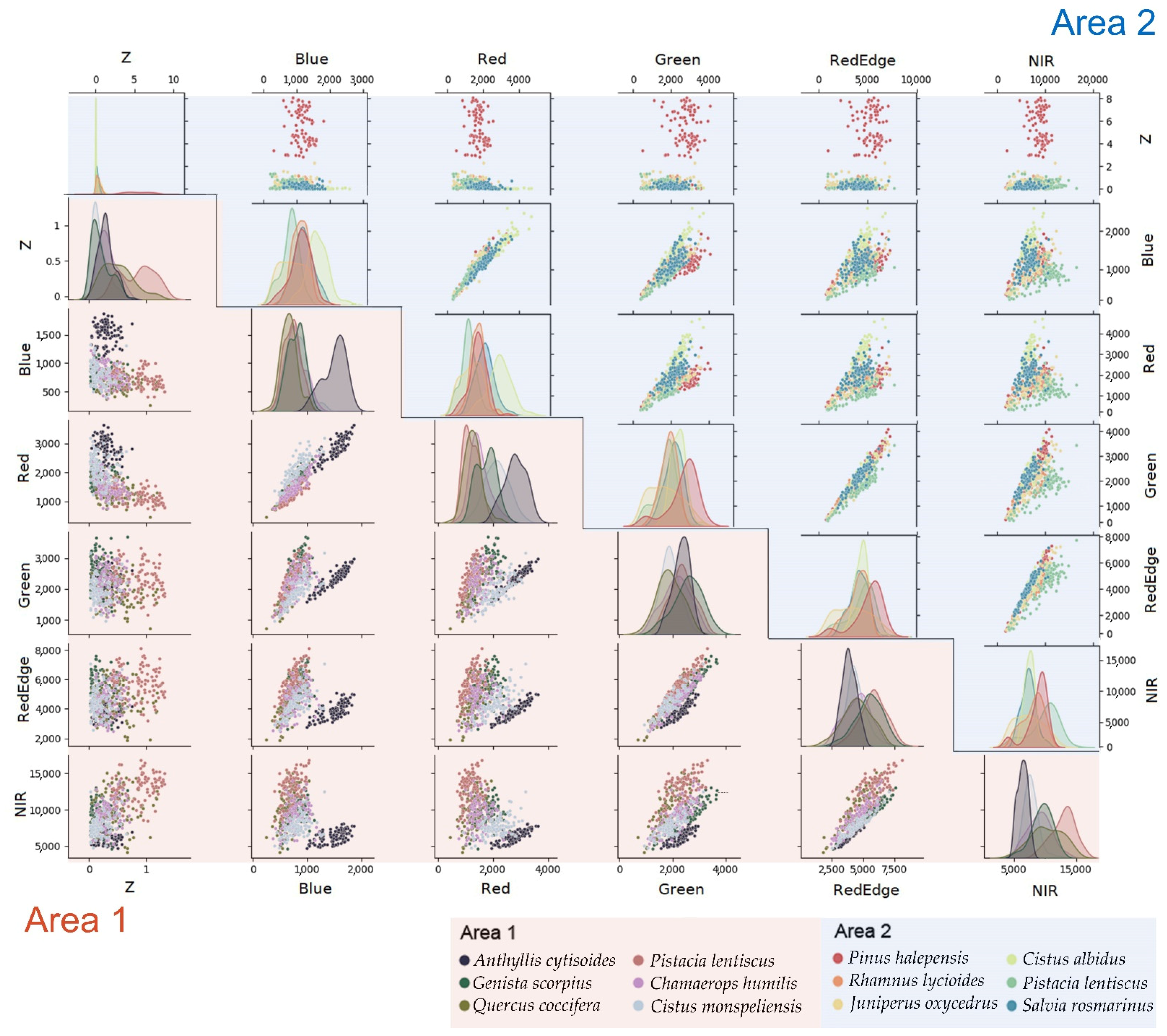
2.6. Feature Extraction

Once the photogrammetric process of obtaining the point cloud and its subsequent normalisation was done, the coordinates (X, Y, Z coordinates) and the reflectance values (blue, green, red, red edge, and near-infrared bands) for each point were stored and 22 spectral features for these points were calculated (

Table 2. Summary of vegetation indices with their respective equations and references; $\mathsf{\rho }$ is defined as the digital number of the point for a given band.

Index (Description)	Equation	Reference
ARVI (Atmospherically Resistant Vegetation Index)	$\left({\mathsf{\rho }}_{nir}-{\mathsf{\rho }}_{rb}\right)/\left({\mathsf{\rho }}_{nir}+{\mathsf{\rho }}_{rb}\right)$$,{ \mathsf{\rho }}_{rb}={\mathsf{\rho }}_{red}-\left[{\mathsf{\rho }}_{blue}-{\mathsf{\rho }}_{red}/2\right]$	[37]
BI (Brightness)	${\mathsf{\rho }}_{green}+{\mathsf{\rho }}_{red}+{\mathsf{\rho }}_{blue}$	[38]
DVI (Differential Vegetation Index)	${\mathsf{\rho }}_{nir}-{\mathsf{\rho }}_{red}$	[39]
EVI (Enhanced Vegetation Index)	$\left[2.5·({\mathsf{\rho }}_{blue}-{\mathsf{\rho }}_{red}\right)]/[({\mathsf{\rho }}_{nir}+6·{\mathsf{\rho }}_{red}-7.5·{\mathsf{\rho }}_{blue}+1)]$	[40]
GNDVI (Green Normalised Difference Vegetation Index)	$({\mathsf{\rho }}_{nir}-{\mathsf{\rho }}_{green})/({\mathsf{\rho }}_{nir}+{\mathsf{\rho }}_{green})$	[41]
GR (Green divided by red)	${\mathsf{\rho }}_{green}/{\mathsf{\rho }}_{red}$	[38]
IPVI (Infrared Percentage Vegetation Index)	${\mathsf{\rho }}_{nir}/({\mathsf{\rho }}_{nir}+{\mathsf{\rho }}_{green})$	[42]
MSAVI (Modified Soil-Adjusted Vegetation Index)	$\left(2·{\mathsf{\rho }}_{nir}+1-{[{\left(2·{\mathsf{\rho }}_{nir}+1\right)}^2-8·\left({\mathsf{\rho }}_{nir}-{\mathsf{\rho }}_{red}\right)]}^{0.5}\right)/2$	[43]
MSR (Modified Simple Ratio Index)	${\mathsf{\rho }}_{red}/{\left({\mathsf{\rho }}_{nir}/{\mathsf{\rho }}_{red}\right)}^{0.5}$	[44]
NDVI (Normalised Difference Vegetation Index)	$\left({\mathsf{\rho }}_{nir}-{\mathsf{\rho }}_{red}\right)/\left({\mathsf{\rho }}_{nir}+{\mathsf{\rho }}_{red}\right)$	[45]
NBRDI (Normalised Blue-Red Difference Index)	$({\mathsf{\rho }}_{red}-{\mathsf{\rho }}_{blue})/({\mathsf{\rho }}_{red}+{\mathsf{\rho }}_{blue})$	[46]
NGBDI (Normalised Green-Blue Difference Index)	$({\mathsf{\rho }}_{green}-{\mathsf{\rho }}_{blue})/({\mathsf{\rho }}_{green}+{\mathsf{\rho }}_{blue})$	[47]
NGRDI (Normalised Green-Red Difference Index)	$({\mathsf{\rho }}_{green}-{\mathsf{\rho }}_{red})/({\mathsf{\rho }}_{green}+{\mathsf{\rho }}_{red})$	[48]
NormG (Normalised Greenness)	${\mathsf{\rho }}_{green}/\left({\mathsf{\rho }}_{green}+{\mathsf{\rho }}_{red}+{\mathsf{\rho }}_{blue}\right)$	[49]
OSAVI (Optimised Soil Adjusted Vegetation Index)	$\left({\mathsf{\rho }}_{nir}-{\mathsf{\rho }}_{red}\right)/\left({\mathsf{\rho }}_{nir}+{\mathsf{\rho }}_{red}+0.16\right)$	[50]
RDVI (Renormalised Difference Vegetation Index)	$\left({\mathsf{\rho }}_{nir}-{\mathsf{\rho }}_{red}\right)/{\left({\mathsf{\rho }}_{nir}+{\mathsf{\rho }}_{red}\right)}^{0.5}$	[51]
RGRI (Red Green Ratio Index)	${\mathsf{\rho }}_{red}/{\mathsf{\rho }}_{green}$	[52]
RVI (Ratio Vegetation Index)	${\mathsf{\rho }}_{red}/{\mathsf{\rho }}_{nir}$	[53]
SARVI (Soil and Atmospherically Resistant Vegetation Index)	$\left[1.5·\left({\mathsf{\rho }}_{nir}-{\mathsf{\rho }}_{rb}\right)\right]/({\mathsf{\rho }}_{nir}+{\mathsf{\rho }}_{red}+0.5)$$,{ \mathsf{\rho }}_{rb}={\mathsf{\rho }}_{red}-\left[{\mathsf{\rho }}_{blue}-{\mathsf{\rho }}_{red}/2\right]$	[54]
SAVI (Soil Adjusted Vegetation Index)	$1.5·\left({\mathsf{\rho }}_{nir}-{\mathsf{\rho }}_{rb}\right)/({\mathsf{\rho }}_{nir}+{\mathsf{\rho }}_{red}+0.5)$	[54]
SR (Simple Ration Vegetation Index)	${\mathsf{\rho }}_{nir}/{\mathsf{\rho }}_{red}$	[55]
SRxNDVI (Simple Ratio × Normalised Difference Vegetation Index)	$\left({\mathsf{\rho }}_{nir}{}^2-{\mathsf{\rho }}_{red}\right)/\left({\mathsf{\rho }}_{nir}+{\mathsf{\rho }}_{red}{}^2\right)$	[56]

).

Finally, we conducted a neighbourhood analysis of each point, determining the neighbourhood of a point as p ∈ R³, with R³ being the set of points inside a sphere s, of centre p, and radius 10 cm. From this neighbourhood analysis 10 features were obtained (

Table 3. Summary of neighbourhood features and equations. S_p is defined as the set of points that form a neighbourhood.

Name (Description)	Equation
Dist_mean (Mean distance of the point with its neighbouring points)	$\overline{d}\left(S_p,p\right)=\frac{1}{n}\left({\displaystyle {\displaystyle \sum }_{i=1}^n}d\left(S_{p,i},p\right)\right)$
Dist_std (Standard deviation of the point with its neighbouring points)	$\sqrt{\frac{[({\sum }_{i=1}^n{(d\left(S_{p,i},p\right)-\overline{d}\left(S_p,p\right))}^2)]/\left(n-1\right)}{n-1}}$
NDVI_mean (Mean NDVI of the point and its neighbouring points)	$\overline{NDVI}\left(S_p\right)=\frac{1}{n}\left({\displaystyle {\displaystyle \sum }_{i=1}^n}NDVI(S_{p_{,i}})\right)$
NDVI_std (Standard deviation NDVI of the point and its neighbouring points)	$\sqrt{\frac{{({\sum }_{i=1}^n(NDVI(S_{p_{,i}})-\overline{NDVI}\left(S_p\right))}^2)}{n-1}}$
Numbers (Number of neighbours)	$n$
Z_mean (Mean height of the point and its neighbours)	$\overline{z}\left(S_p\right)=\frac{1}{n}\left({\displaystyle {\displaystyle \sum }_{i=1}^n}(z(S_{p_{,i}})\right)$
Z_std (Standard deviation height of the point and its neighbours)	$\sqrt{\frac{{({\sum }_{i=1}^n(z(S_{p_{,i}})-\overline{z}\left(S_p\right))}^2)}{n-1}}$
Dif_Z (Maximum height of the neighbourhood minus minimum height of the neighbourhood)	$\max \left(z(S_p)\right)-\min \left(z\left(S_p\right)\right)$
Z_Zmin (Height of the point minus neighbourhood minimum height)	$z\left(p\right)-\min \left(z\left(S_p\right)\right)$
Zmax-Z (Maximum height of the neighbourhood minus height of the point)	$\max \left(z(S_p)\right)-z\left(p\right)$

).

2.7. Machine and Deep Learning Models

To carry out the point cloud classification by species, we performed a supervised classification of the point cloud, also known as point cloud semantic segmentation [57]. The training samples used to fit the models were extracted from field work data, where different geolocated individuals of each species were identified. A planimetric buffer of 15 cm was applied to these geolocated points, with this value being the minimum radius of the smallest individuals identified. The resulting polygon was used to clip the point cloud. After obtaining the samples for each class (Table 1), a process of manual filtering was conducted to avoid the introduction of outliers in the training samples. Figure 4 shows a representation of the training samples of each species based on some features extracted from the point cloud. This figure is a pairwise relationship plot of the dataset created from 100 random points of each of the species studied with their raw spectral bands and normalised height. It can be seen from the Kernel Density Estimator (KDE) located on the diagonals how in area 1 the species Anthyllis cytisoides differs from the others in the blue and red bands or how the species Pistacia lentiscus can be differentiated using only the normalised height information. This figure also shows the difficulty in distinguishing some species studied on the basis of these features. For example, in area 2 we found that the species Cistus albidus and Salvia rosmarinus have a similar spectral response and normalised height, making them difficult to differentiate. The relationships established in the upper and lower corners help to visualise the similarity or the difference between species. On the basis of its spectral features, the best distinguished species in area 1 was Anthyllis cytisoides, while the rest of the species were difficult to differentiate. In area 2, the normalised height was the feature that best distinguishes the Pinus halepensis species, while the spectral response of the different species was similar. In summary, Figure 4 shows that all studied species cannot be distinguished from each other on the basis of their raw spectral features and their height, making an in-depth analysis necessary.

Different machine learning and deep learning methods were evaluated for this classification, using the Python library Scikit-learn [58]. The machine learning methods evaluated were DT [59], Extra Trees [60], Gradient Boosting [61], and Random Forest [62], as well as the deep learning method MultiLayer Perceptron [63]. For the evaluation of these methods, a fine-tuning of the hyperparameters (

Table 4. Hyperparameters used in the models’ fine-tuning.

Model	Hyperparameter #1 (Values)	Hyperparameter #2 (Values)	Hyperparameter #3 (Values)	Hyperparameter #4 (Values)
Decision Tree Extra Trees Gradient Boosting	Maximum depth of the tree (5, 10, None)	Minimum number of samples required to split an internal node (2, 3, 5)	Minimum number of samples required to be at a leaf node (1, 2, 5)	-
Random Forest	Number of trees in the forest (200, 500)	Number of features to consider (‘auto’, ‘sqrt’, ‘log2’)	Maximum depth of the tree (4, 5, 6, 7, 8)	Function to measure the quality of a split (‘gini’, ‘entropy’)
MultiLayer Perceptron	Number of neurons in the ith hidden layer (50, 50, 50), (50, 100, 50), (100)	Activation (‘tanh’, ‘relu’)	Solver (‘sgd’, ‘adam’)	Alpha (0.0001, 0.05)

) was done with the aim of optimizing the models. This fine-tuning was carried out by setting up a grid of hyperparameters. The accuracy of each combination of hyperparameters was assessed by cross-validation with 10-fold to ensure the independence between training and test data. The chosen hyperparameters for each method were those with the highest mean cross-validated score (mCVs). For the selection of the point cloud classification method, the mCVs of each method were also considered.

After selecting the model, feature selection was applied with the aim of reducing the number of features in the final model to avoid overfitting. This feature selection was based on the permutation feature importance of the fitted model as well as the Pearson correlation between features. The permutation feature importance is based on the decrease in the score of a model when a single feature value is randomly shuffled [62]. Using this technique, the features in each area were ordered based on their permutation feature importance value. The Pearson correlation of the features was then calculated, and the features were split into clusters. Each feature, ordered according to its feature importance, was assigned a weight that decreased according to the repeatability of the cluster to which it belonged. Therefore, even if a feature had a high feature importance, if features from the same cluster with higher importance had been selected, the latter might not be selected. After the feature extraction, a classification was done again with the chosen features, using the same classification method used previously.

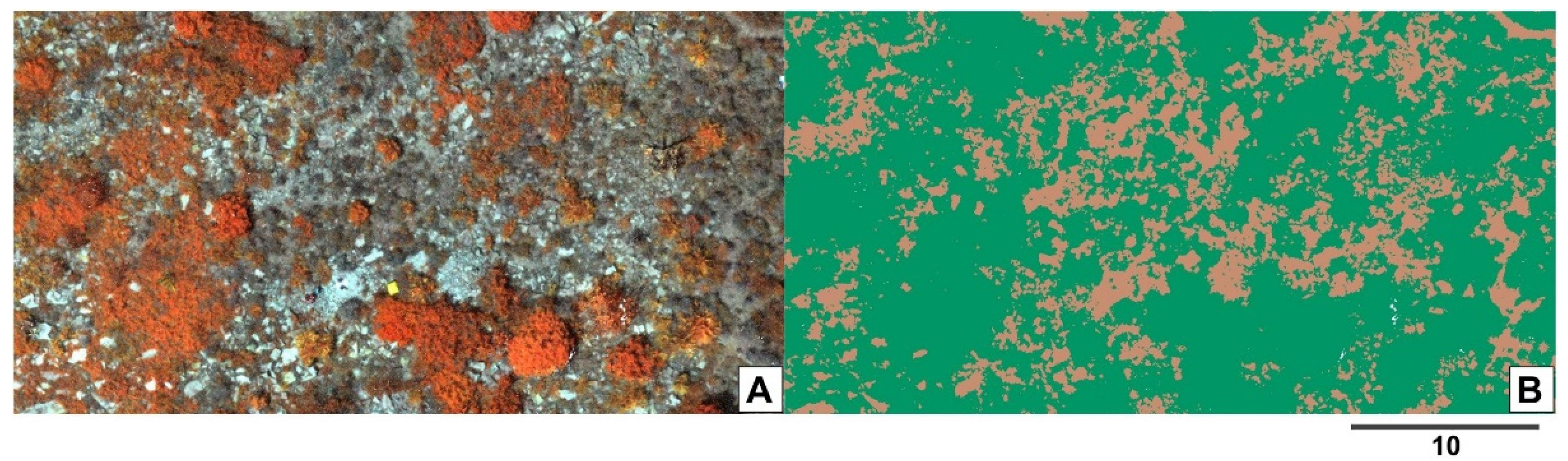
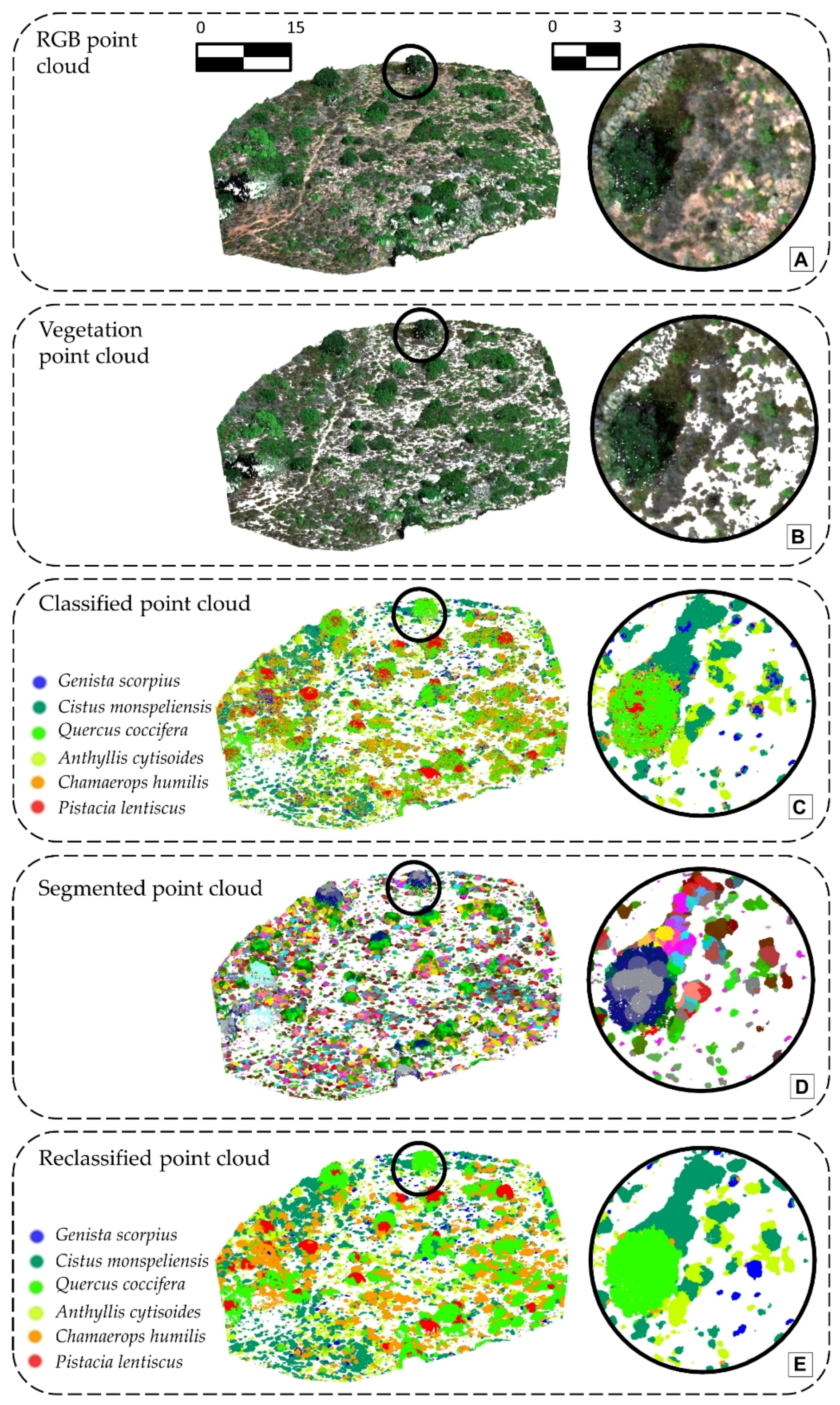
2.8. Point Cloud Segmentation and Reclassification

After finding the model that best fit the training samples and predicting the class of each point, the high spatial heterogeneity of the classified point cloud was reduced by performing a geometric segmentation of the point cloud, with the aim of obtaining point clusters representing different individuals. We applied the algorithm li2012 [64] from the lastrees function of lidR package [65]. This algorithm is based on region growing to determine whether a point is near or far from existing vegetation, taking advantage of the relative separation between objects to discern between individuals. To achieve the objective of containing only one individual per segment, the algorithm was parameterised to perform an over-segmentation, favouring that there were no segments containing two or more individuals of different species. The selected parameters for segmenting the point clouds were: threshold 1 = 0.1 m, threshold 2 = 0.2 m, limit of threshold number 1 = 1.5 m, minimum height of a detected tree = 0.01 m, maximum radius of a crown is 1 m, and search radii = 0.1 m and 0.5 m, respectively, for areas 1 and 2. After segmenting the point cloud, each segment was assigned the most repeated class to increase the spatial homogeneity of the point classification.

2.9. Evaluation

For evaluation purposes, we manually segmented and classified different individuals of each species to create the testing set. These point clouds were taken as a reference for an accuracy assessment of the point classification performed. The evaluation was done by comparing the class obtained from each point with the reference class. The confusion matrix of the reference samples was obtained, as well as the precision (Pr), recall (Re), and F-measure (Fm) values from the following equations.

$$\mathrm{A}=\left[\begin{array}{cccc}{\mathrm{a}}_{1,1}& {\mathrm{a}}_{1,2}& \dots & {\mathrm{a}}_{1,\mathrm{j}}\\ {\mathrm{a}}_{2,1}& {\mathrm{a}}_{2,2}& \dots & {\mathrm{a}}_{2,\mathrm{j}}\\ \dots & \dots & \dots & \dots \\ {\mathrm{a}}_{\mathrm{i},1}& {\mathrm{a}}_{\mathrm{i},2}& \dots & {\mathrm{a}}_{\mathrm{i},\mathrm{j}}\end{array}\right]$$

(1)

$${\mathrm{TP}}_{\mathrm{i}}={\mathrm{a}}_{\mathrm{i},\mathrm{j}}$$

(2)

$${\mathrm{FP}}_{\mathrm{i}}={\displaystyle \sum }_1^{\mathrm{i}}{\mathrm{a}}_{\mathrm{j},\mathrm{i}}-{\mathrm{TP}}_{\mathrm{i}}$$

(3)

$${\mathrm{FN}}_{\mathrm{i}}={\displaystyle \sum }_1^{\mathrm{i}}{\mathrm{a}}_{\mathrm{i},\mathrm{j}}-{\mathrm{TP}}_{\mathrm{i}}$$

(4)

$$\mathrm{Pr}=\frac{\mathrm{TP}}{\mathrm{TP}+\mathrm{FP}}$$

(5)

$$\mathrm{Re}=\frac{\mathrm{TP}}{\mathrm{TP}+\mathrm{FN}}$$

(6)

$$\mathrm{Fm}=2·\frac{\mathrm{Pr}·\mathrm{Re}}{\mathrm{Pr}+\mathrm{Re}}$$

(7)

where A represents the confusion matrix, TP is True Positives, FP is False Positives, FN is False Negatives, Pr is the precision, Re is the recall, and Fm is the F-measure.

3. Results and Discussion

Figure 5 shows a summary of the intermediate results to obtain the classified point cloud. Firstly, the point cloud was obtained, normalised, and the bare ground points were removed. The normalised point cloud was classified using six species’ classes. Subsequently, the point cloud was segmented according to its geometry to perform a reclassification that homogenised the previously performed classification.

3.1. Generation and Processing of the Point Clouds

The point cloud obtained for Area 1 was composed of 4,107,175 points with an average density of 1421.5 points·m⁻², whereas the point cloud for Area 2 was composed of 11,514,975 points with an average density of 1005.3 points·m⁻². Their positional error was estimated through the Root Mean Square Error (RMSE) between the GCPs and the position of the computed 3D point, being 3.45 cm for Area 1 and 3.79 cm for Area 2.

Regarding the Random Forest classification of the UAV-DAP point cloud to separate bare ground and vegetation points, with respect to the results obtained in each of the iterations carried out using cross-validation, a mCVs of 0.998 and a standard deviation of cross-validated score (stdCVs) of 0.004 were obtained for Area 1. For Area 2, a mCVs of 0.999 and a stdCVs of 0.003 were obtained.

Prior to the merging of the UAV-DAP and ALS bare ground points, we performed a statistical analysis of the point clouds. In order to compare the correct alignment of the UAV-DAP and ALS bare ground points, the nearest neighbour distance of each point between both clouds was calculated. Analysing the distances in the Z-component, a mean distance of −3.4 cm and a standard deviation of 10.6 cm were obtained for Area 1; for Area 2, these values were 1.8 cm and 21.2 cm, respectively. The high standard deviation was due to two reasons: The main one was the discontinuity of the ground in the UAV-DAP point cloud due to gaps caused by vegetation; the second one was the accuracy in the Z component of the methods, 3.2 cm for the UAV-DAP (measured in the GCPs) and 15 cm for the ALS point cloud. The use of the ALS reduced the gaps in the points classified as ground, adding information where photogrammetric clouds were limited due to the reduced penetration of UAV-DAP data through vegetation.

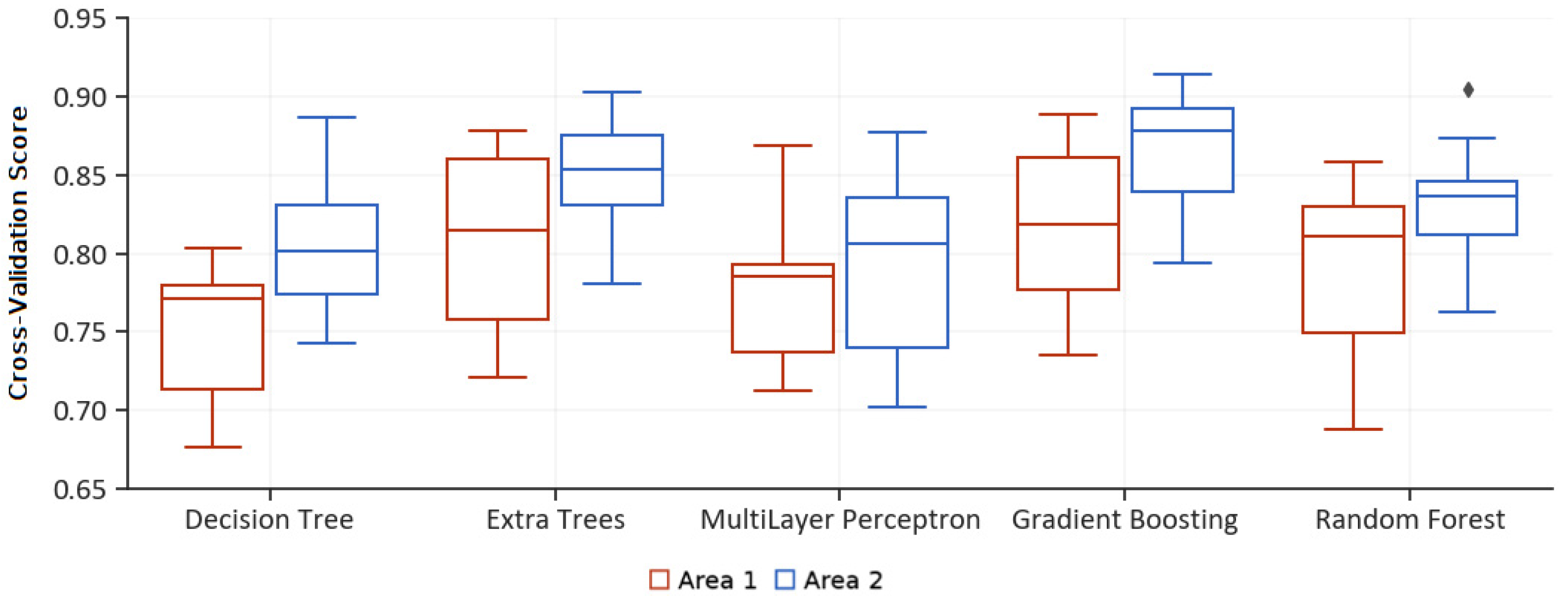
3.2. Assessment of Classification Methods

The selection of the classifier among the different methods analysed (Decision Tree, Extra Trees, MLP, Gradient Boosting, and Random Forest) was based on their cross-validation results applying the hyperparameters that best adapted to the training samples of vegetation species. The model that achieved the highest reliability and lowest dispersion was Gradient Boosting (Figure 6), both for Area 1 and Area 2. In both areas, the model with the highest reliability for a unique k-fold was also Gradient Boosting with 0.89 and 0.95, for the study areas 1 and 2, respectively. Analysing the set of repetitions, Gradient Boosting obtained higher average accuracy values with lower dispersion (0.82 ± 0.05 and 0.91 ± 0.02 mean and standard deviation of cross-validation score for study Area 1 and 2, respectively). In this respect, there were slight differences between Gradient Boosting and Extra trees (0.81 ± 0.06 and 0.90 ± 0.02 mean and standard deviation of cross-validation score for study Area 1 and 2, respectively). Using Decision Trees, MultiLayer Perceptron, and Random Forest, less accurate results were obtained. Regardless of the classifier used, more accurate results were obtained for Area 2, since the species analysed in Area 1 had a greater geometric and spectral similarity compared to the species analysed in Area 2 (Figure 4). In this sense, other studies obtained similar results when classifying UAV-DAP point clouds using geometric and spectral features [66]. In this study, Random Forest and Gradient boosting classifiers were compared, finding that the classifier with the lowest error was also Gradient Boosting. The results are also comparable to those obtained classifying satellite images, where the Gradient Boosting classifier outperformed different deep neural networks and other machine learning classifiers using spectral, spatial, textural, and vegetation index features [67]. Similar results were obtained in [68], where the methods Regression Trees, Random Forest, and Gradient Boosting were compared to classify forest fuel types from ALS data and satellite imagery, concluding that the best results were obtained using Gradient Boosting.

Table 5. Heatmap of the hyperparameters (minimum number of samples at a leaf node, minimum number of samples to split an internal node, and maximum depth of the tree) applied to the Gradient Boosting method. The table shows the mean cross-validated scores obtained over 10 iterations and the mean fit time used in their calculation. The red gradient is associated with Area 1 values, while the blue gradient represents values from Area 2.

		Area 1						Area 2
		Mean Cross-Validated Score			Mean Fit Time (s)			Mean Cross-Validated Score			Mean Fit Time (s)
Minimum number of samples at a leaf node	1	0.745	0.757	0.781	1347	1473	1814	0.891	0.894	0.901	5985	5859	6516	None	Maximum depth of the tree
	2	0.793	0.792	0.797	1698	1684	1568	0.908	0.908	0.909	5968	5966	5820
	5	0.809	0.810	0.809	1109	1110	1033	0.914	0.915	0.914	4967	4969	4601
	1	0.819	0.818	0.818	258	256	256	0.910	0.911	0.912	695	702	703	5
	2	0.818	0.821	0.819	256	255	255	0.911	0.911	0.910	707	703	697
	5	0.820	0.819	0.819	255	254	258	0.912	0.912	0.911	705	726	743
	1	0.812	0.812	0.810	487	483	469	0.913	0.913	0.914	1395	1344	1291	10
	2	0.811	0.812	0.812	467	464	462	0.913	0.914	0.914	1294	1298	1298
	5	0.817	0.817	0.815	460	471	496	0.915	0.915	0.914	1317	1344	1340
		2	3	5	2	3	5	2	3	5	2	3	5
		Minimum number of samples to split an internal node

shows the results of the different combinations of hyperparameters applied to the Gradient Boosting method. The combination of parameters that obtained the highest mCVs for Area 1 was the one formed by the minimum number of samples required to split an internal node of 3, minimum number of samples required to be at a leaf node of 2, and a maximum depth of the tree of 5, with a mean fit time of 255 s for each of the 10 iterations. On the other hand, the highest mCVs for the second area was obtained by the combination of a minimum number of samples required to split an internal node of 2, minimum number of samples required to be at a leaf node of 5, and a maximum depth of the tree of 10, with a mean fit time of 1317 s. Table 5 also shows how the hyperparameter with the greatest influence on the processing time was the maximum depth of the tree, multiplying up to 8 times the time by setting the value to “none”, compared to value “5”, without affecting the improvement of the model. If value is set to “none”, the nodes are expanded until all leaves are pure or until all leaves contain less than the minimum number of samples to split an internal node, which explains the increase in processing time. In contrast, if we analyse the minimum number of samples at a leaf node, the best results were obtained mostly by setting this hyperparameter to “5”.

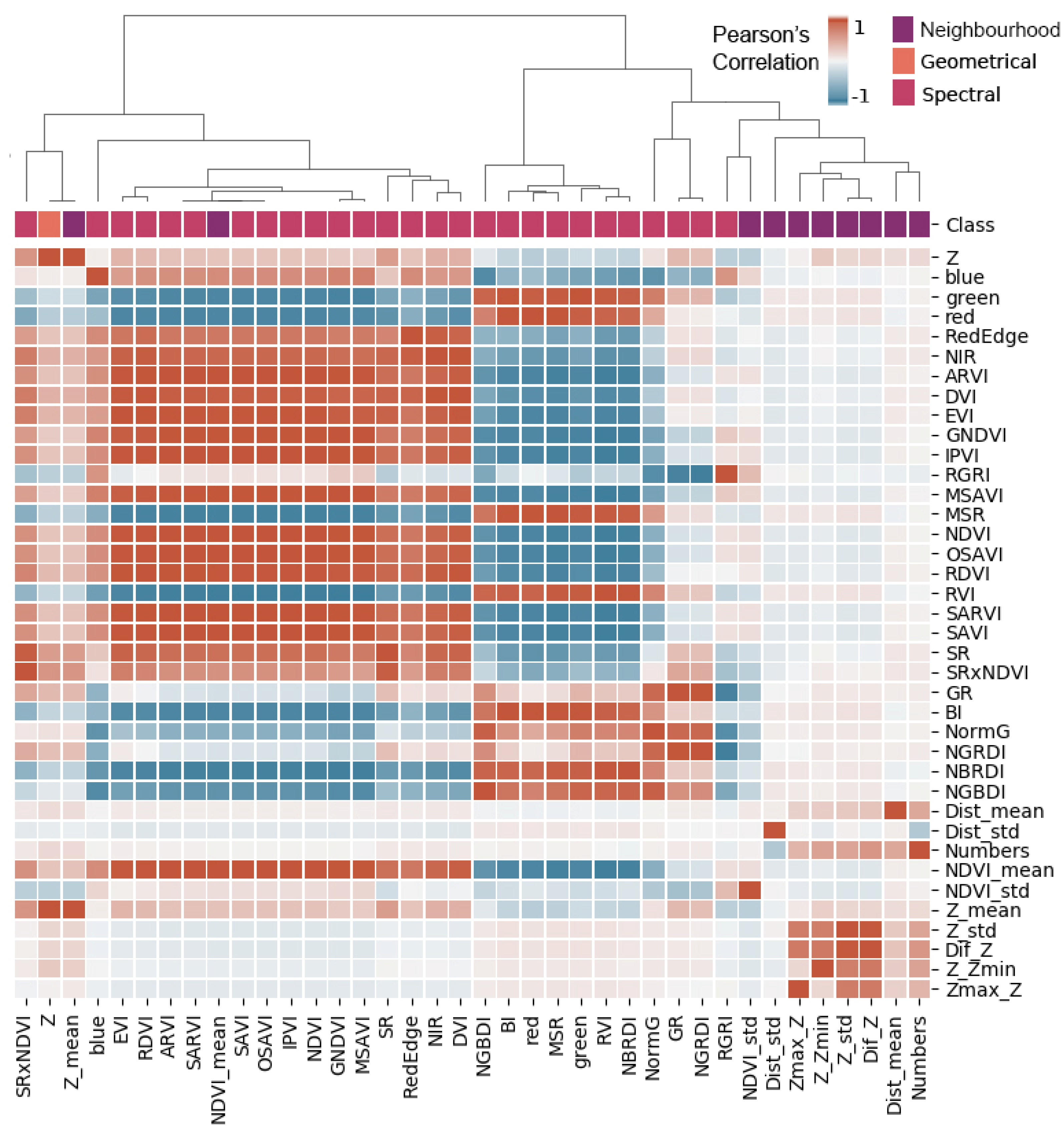
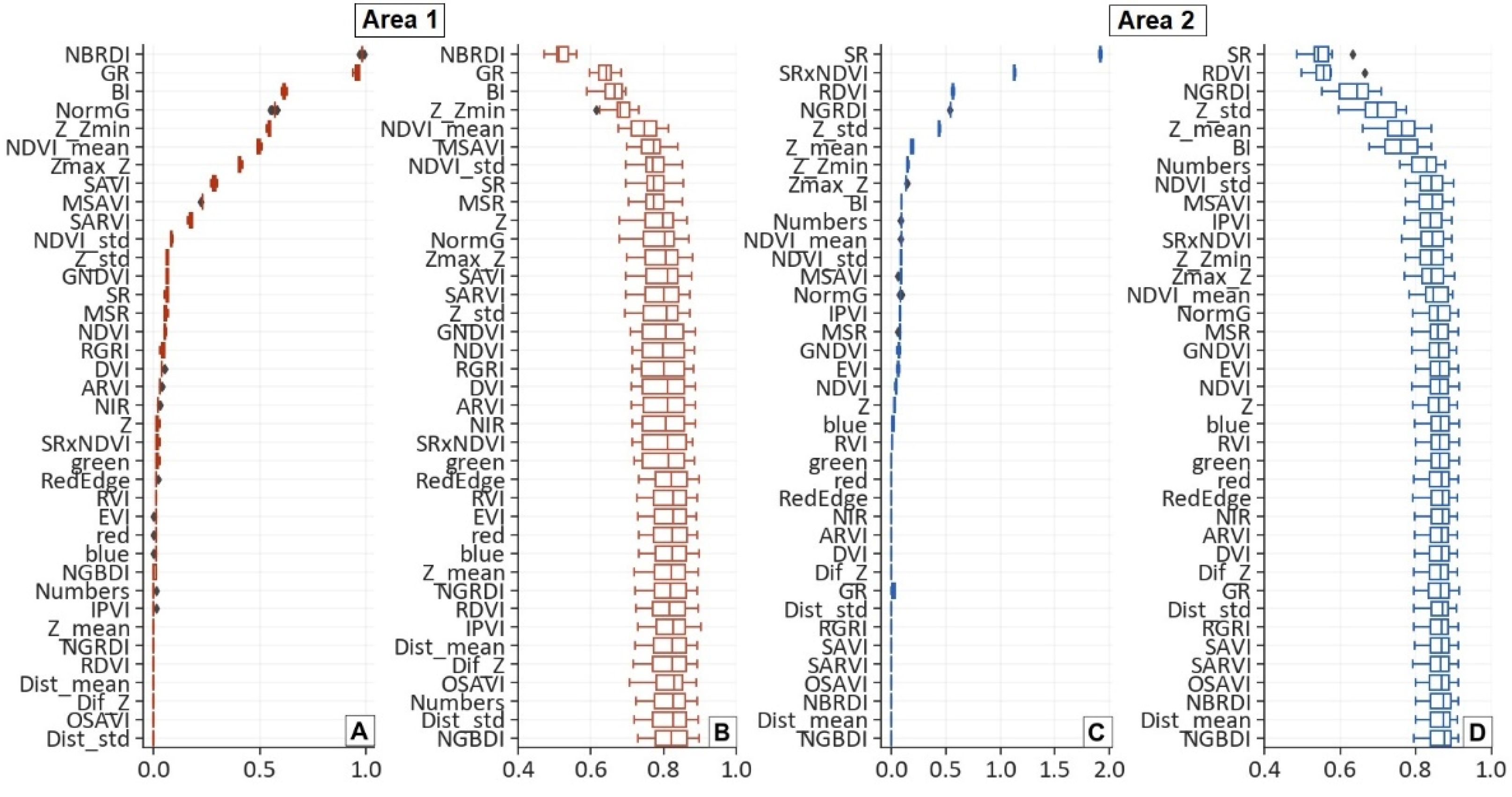
3.3. Feature Selection and Final Classification Model

Once the classifier that best suited our study, gradient boosting, was selected, we applied the feature selection process. To reduce the number of features, we obtained Pearson’s correlation for both areas 1 and 2. Figure 7 shows the existing correlation between features for Area 1, showing the high correlation between spectral features. These features were not directly removed since our first objective was to discern which spectral indices were most important in the classification. Subsequently, the most correlated and least informative features were removed to obtain the final model. Thus, we evaluated the features based on their ability to differentiate between tree and shrub species. From the hierarchical clustering tree, which groups the features based on their Pearson’s correlation, it can be observed that there were five clusters of features. The first was formed by the geometric feature Z and a geometric feature extracted from the neighbourhood analysis, the feature Z_mean. The second cluster was formed by 17 features, all of them spectral features except the NDVI_mean, with this being a spectral feature extracted from the neighbourhood analysis; in this cluster are also SRxNDVI, blue, EVI, RDVI, ARVI, SARVI, SAVI, OSAVI, IPVI, NDVI, GNDVI, MSAVI, SR, RedEdge, NIR, and DVI. The third cluster consisted entirely of the spectral features NGBDI, BI, red, MSR, green, RVI, and NBRDI. The fourth cluster was mainly composed of spectral features. These features had maximum correlation in absolute value with the spectral features NormG, GR, NGRDI, and RGRI. The last cluster consisted entirely of features extracted from the neighbourhood analysis: Dist_std, Zmax_Z, Z_Zmin, Z_std, Dif_Z, Dist_mean, and Numbers.

Analysing the permutation importance of the features when applying the model (Figure 8A,C), among the top 10 features with the highest permutation importance for the model, three were repeated in the two study areas. These features were one of spectral type, BI, and two extracted from the neighbourhood analysis, Z_Zmin and Zmax_Z. In this sense, we can also observe how, depending on the area, the features with greater importance diverged. In Area 1 the most important feature was the NBRDI index, but in Area 2 this feature was the second to last in order of importance. Since each area has different tree and shrub species, with only one species in common, the common features with high importance values in both areas could be considered as adequate descriptors to differentiate the Mediterranean flora.

Depending on the cluster they belonged to, a weight was applied to the features, modifying their order of importance. The learning curves in Figure 8 show the final order applied to the model. Visualising the learning curve, it stabilised from 10 features onwards for Area 1 (NBRDI, GR, BI, Z_Zmin, NDVI_mean, MSAVI, NDVI_std, SR, MSR, and Z) and Area 2 (SR, RDVI, NGRDI, Z_stf, Z_mean, BI, NUMBERS, NDVI_std, MSAVI, and IPVI), obtaining a slight increase in the mCV statistic by using 38 features instead of 10.

Analysing the decreasing trend in the importance of the features and the stabilisation of the learning curve in both areas, only 10 predictor features were used to obtain the model. In particular, the first 10 features, as shown in Figure 8B,D, were used to create the final classification. Some of these features, such as SR or BI, were also reported as relevant in other models applied for tree species’ classification using UAV-DAP data [69].

3.4. Vegetation Classification Accuracy

Once the points were reclassified, the point cloud was compared with the testing data set, obtaining the confusion matrix shown in

Table 6. Species’ classification confusion matrix with precision (Pr), recall (Re), and F-measure (Fm) for the different classes. Values indicate the number of points collected involved in the evaluation. Column headers are class labels, rows refer to class indices. The red gradient is associated with Area 1 values, while the blue gradient represents values from Area 2.

		Classified as
		Area 1						Area 2
		Genista scorpius	Cistus monspeliensis	Quercus coccifera	Anthyllis cytisoides	Chamaerops humilis	Pistacia lentiscus	Cistus albidus	Rhamnus lycioides	Cade juniper	Pinus halepensis	Pistacia lentiscus	Salvia Rosmarinus
Truth	1	4816	137	0	0	42	0	4516	239	315	317	229	1215
	2	773	15,198	1579	184	850	303	0	16,077	469	185	1095	808
	3	4	476	41,342	0	482	12,567	0	4994	54,185	5085	13,381	3014
	4	98	979	25	6660	213	44	21	566	1431	1,110,973	2012	316
	5	1016	1128	3714	53	24,663	5327	4	124	136	961	59,607	37
	6	0	0	613	0	0	45,833	598	4250	4364	46	1537	46,186
	Pr	0.72	0.85	0.87	0.97	0.94	0.72	0.88	0.61	0.89	0.99	0.77	0.90
	Re	0.96	0.80	0.75	0.83	0.69	0.99	0.66	0.86	0.67	1.00	0.98	0.81
	Fm	0.82	0.83	0.81	0.89	0.79	0.83	0.75	0.72	0.77	1.00	0.86	0.85

. The classification results had an overall accuracy of 81.9% in Area 1 and 96.4% in Area 2. These results were highly dependent on the number of samples taken from each class (Table 1). It was, therefore, necessary to carry out an individual study of each species. Analysing the results in depth, the highest values for user’s accuracy (precision) and F-measure for Area 1 were obtained for the class Anthyllis cytisoides (0.97 and 0.89, respectively). Figure 4 shows how the Anthyllis cytisoides had a differentiated spectral response in the blue and red bands, compared to the rest of the species analysed in Area 1. In relation to Area 2, the highest values for precision, recall, and F-measure were obtained for class Pinus halepensis, achieving values of 0.99, 1.00, and 1.00, respectively. These results are attributed to the fact that it was the only tree species in the area, with the height of all individuals of this species being much greater than that of other species.

The statistics obtained for the Pistacia lentiscus class were remarkable, as it was the only class present in both study areas. In the two areas, we found similar values of recall (0.99 and 0.98, respectively, for areas 1 and 2), precision (0.72 and 0.77), and F-measure (0.83 and 0.86). These lower values were due to confusion with other species, such as Quercus coccifera or Chamaerops humilis in the Area 1 or the Juniperus oxycedrus in Area 2. The Pistacia lentiscus has a high intraspecies’ variability depending on the age (Table 1), causing confusion between the different classes in both study areas. This also explains the relative low recall value for the species Chamaerops humilis (0.69) in Area 1 or Juniperus oxycedrus (0.67) in Area 2. Due to the low number of Pistacia lentiscus individuals, it was not possible to create two classes; but it would be recommended to split this class according to their age (young and mature) in further studies.

The low recall (0.66) of Cistus albidus in Area 2 was due to its misclassification with Salvia rosmarinus. Both species showed spectral and shape similarity, as described in Table 1. Rhamnus lycioides was also confused with Salvia rosmarinus and Juniperus oxycedrus.

The results obtained are comparable with other studies where species’ classification was carried out based on UAV-DAP data. The study performed by Nevalainen et al. [27] allowed for the classification of four boreal forest tree species. They applied k-nearest neighbours, Random Forest, and MultiLayer Perceptron using hyperspectral imagery and UAV-DAP point cloud features. The last two classifiers obtained 95% of overall accuracy. These accurate results can be explained considering the low number of species analysed compared to our study. Tuominen et al. [33] performed a more challenging study using a similar methodology. Their methodology was based on the analysis of k-nearest neighbours and Random Forest classifiers, using also UAV-DAP point clouds and hyperspectral image mosaics for classifying 26 different tree species in southeastern Finland. The highest global accuracy was obtained for the classifier k-nearest neighbours, with a global accuracy of 82%. Depending on the species analysed, producer and user accuracies ranged from 0% to 100%. Sothe et al. [28] obtained a classification of 12 major tree species in a subtropical forest integrating UAV-DAP point cloud and hyperspectral data and applying a support vector machine classifier. The overall accuracy obtained in this study was 72%. All these studies have in common that the final product is a classification map, being able to extract from it only two-dimensional information (e.g., the location of the trees or the perimeter of their crown). This short literature review highlights the results obtained in this work, where 11 different tree and shrub species were classified using multispectral information. The analysis of the point cloud and the extraction of geometric and neighbourhood features allowed us to differentiate species with a similar spectral response. In addition, the classified point cloud allowed the derivation of information on the forest structure that can be used as input for wildfire models.

3.5. Improving Wildfire Behaviour Modelling

The present study achieved a new methodology to classify Mediterranean forest species from UAV point clouds with the aim of improving wildfire behaviour modelling. Current wildfire models need to be fed with 3D fuel data for their correct running. These computational models need information about the geometry of the individuals (adapting it to a geometric body) and their properties (e.g., fuel density, surface–volume ratio, or fuel moisture) [70]. These properties are inherent to the species analysed, making a prior classification of the study area necessary. Individual point clouds can be adjusted to a geometric body, as well as obtaining individual properties using allometric equations. These equations describe the relationship between variables extracted directly from the point cloud (e.g., tree height, area, volume, or crown width) with the properties required as input by the wildfire models (e.g., bulk density) [14]. Therefore, the use of UAVs for the characterisation of forest structure allows for a breakthrough in the improvement of wildfire models; being able to identify tree and shrub individuals by semi-automatic species identification is one of the key parameters to be used in fire models.

4. Conclusions

This investigation developed and proposed a UAV-DAP method for the classification of forest species. Results were very promising, showing that UAV-DAP points clouds have the potential to provide accurate results in species’ classification. The spectral, geometrical, and neighbourhood features derived from multispectral images produced good results classifying shrub and tree species.

To the best of the authors’ knowledge, this is one of the first investigations studying the classification of shrub and tree species in Mediterranean forests using multispectral imagery obtained from UAVs. Previous studies have not proposed similar objectives using only a multispectral camera and a consumer drone, which highlights the methodology proposed in this article, which can be exported to other fields. The proposed methodology allows for scalability of the area and number of species to be studied. In this sense, if the number of species increases, there may be some geometric or spectral similarities among those species, making it necessary to increase the spectral resolution of the input data to improve the results. Due to the results obtained, and to previous articles using similar features for the classification of species, some of the features proposed in this article are relevant in the classification of Mediterranean shrub and tree species.

The classified point cloud provides valuable input to the wildfire models. Obtaining a classified point cloud can lead to the automatic extraction of different features by species (height, area, volume, crown width, etc.), allowing the estimation of variables such as bulk density using allometric equations, which are key for the correct parameterisation of wildfire models.

References

1. Velez, R.; Salazar, M.; Troenesgaard, J.; Saigal, R.; Wade, D.D.; Lundsford, J. Fire. Unasylva (Engl. Ed.) 1990, 41, 3–38. [Google Scholar]
2. Botella-Martínez, M.A.; Fernández-Manso, A. Study of post-fire severity in the Valencia region comparing the NBR, RdNBR and RBR indexes derived from Landsat 8 images. Rev. Teledetecc. 2017, 49, 33–47. [Google Scholar] [CrossRef] [Green Version]
3. Attiwill, P.M. The disturbance of forest ecosystems: The ecological basis for conservative management. For. Ecol. Manag. 1994, 63, 247–300. [Google Scholar] [CrossRef]
4. Lionello, P.; Scarascia, L. The relation between climate change in the Mediterranean region and global warming. Reg. Environ. Chang. 2018, 18, 1481–1493. [Google Scholar] [CrossRef]
5. Pausas, J.G.; Fernández-Muñoz, S. Fire regime changes in the Western Mediterranean Basin: From fuel-limited to drought-driven fire regime. Clim. Chang. 2012, 110, 215–226. [Google Scholar] [CrossRef] [Green Version]
6. Turco, M.; Rosa-Cánovas, J.J.; Bedia, J.; Jerez, S.; Montávez, J.P.; Llasat, M.C.; Provenzale, A. Exacerbated fires in Mediterranean Europe due to anthropogenic warming projected with non-stationary climate-fire models. Nat. Commun. 2018, 9, 1–9. [Google Scholar] [CrossRef]
7. Williams, C.; Biswas, T.; Black, I.; Harris, P.; Heading, S.; Marton, L.; Czako, M.; Pollock, R.; Virtue, J. Use of poor quality water to produce high biomass yields of giant reed (Arundo donax L.) on marginal lands for biofuel or pulp/paper. Acta Hortic. 2009, 806, 595–602. [Google Scholar] [CrossRef]
8. López-Santalla, A.; López-Garcia, M. Los Incendios Forestales en España. Decenio 2006–2015; Ministerio de Agricultura Pesca y Alimentación: Madrid, Spain, 2019.
9. WWF España. Arde el Mediterráneo; WWF/Adena: Madrid, Spain, 2019. [Google Scholar]
10. Campo, J. Efectos de Incendios Experimentales Repetidos en la Agregación del Suelo y su Evolución Temporal. Ph.D. Thesis, Universidad de Valencia España, Valencia, Spain, 2012. [Google Scholar]
11. Giorgi, F. Climate change hot-spots. Geophys. Res. Lett. 2006, 33, L08707. [Google Scholar] [CrossRef]
12. Oliveira, S.; Rocha, J.; Sá, A. Wildfire risk modeling. Curr. Opin. Environ. Sci. Health 2021, 23, 100274. [Google Scholar] [CrossRef]
13. Bakhshaii, A.; Johnson, E.A. A review of a new generation of wildfire–atmosphere modeling. Can. J. For. Res. 2019, 49, 565–574. [Google Scholar] [CrossRef] [Green Version]
14. Shin, P.; Sankey, T.; Moore, M.; Thode, A. Evaluating Unmanned Aerial Vehicle Images for Estimating Forest Canopy Fuels in a Ponderosa Pine Stand. Remote Sens. 2018, 10, 1266. [Google Scholar] [CrossRef] [Green Version]
15. Mell, W.; Jenkins, M.A.; Gould, J.; Cheney, P. A physics-based approach to modelling grassland fires. Int. J. Wildl. Fire 2007, 16, 1–22. [Google Scholar] [CrossRef]
16. Stratton, R.D. Assessing the effectiveness of landscape fuel treatments on fire growth and behavior. J. For. 2004, 102, 32–40. [Google Scholar]
17. Linn, R.; Reisner, J.; Colman, J.J.; Winterkamp, J. Studying wildfire behavior using FIRETEC. Int. J. Wildl. Fire 2002, 11, 233–246. [Google Scholar] [CrossRef]
18. Keane, R.E. Wildland Fuel Fundamentals and Applications; Springer: Missoula, MT, USA, 2015; ISBN 3319090151. [Google Scholar]
19. Rollins, M.G. LANDFIRE: A nationally consistent vegetation, wildland fire, and fuel assessment. Int. J. Wildl. Fire 2009, 18, 235–249. [Google Scholar] [CrossRef] [Green Version]
20. Kerr, J.T.; Ostrovsky, M. From space to species: Ecological applications for remote sensing. Trends Ecol. Evol. 2003, 18, 299–305. [Google Scholar] [CrossRef]
21. De Cáceres, M.; Casals, P.; Gabriel, E.; Castro, X. Scaling-up individual-level allometric equations to predict stand-level fuel loading in Mediterranean shrublands. Ann. For. Sci. 2019, 76, 1–17. [Google Scholar] [CrossRef]
22. Pyne, S.J. Introduction to Wildland Fire. Fire Management in the United States; John Wiley & Sons: New York, NY, USA, 1984; ISBN 047109658X. [Google Scholar]
23. Crespo-Peremarch, P.; Tompalski, P.; Coops, N.C.; Ruiz, L.Á. Characterizing understory vegetation in Mediterranean forests using full-waveform airborne laser scanning data. Remote Sens. Environ. 2018, 217, 400–413. [Google Scholar] [CrossRef]
24. Fassnacht, F.E.; Latifi, H.; Stereńczak, K.; Modzelewska, A.; Lefsky, M.; Waser, L.T.; Straub, C.; Ghosh, A. Review of studies on tree species classification from remotely sensed data. Remote Sens. Environ. 2016, 186, 64–87. [Google Scholar] [CrossRef]
25. Iglhaut, J.; Cabo, C.; Puliti, S.; Piermattei, L.; O’Connor, J.; Rosette, J. Structure from motion photogrammetry in forestry: A review. Curr. For. Rep. 2019, 5, 155–168. [Google Scholar] [CrossRef] [Green Version]
26. Paneque-Gálvez, J.; McCall, M.K.; Napoletano, B.M.; Wich, S.A.; Koh, L.P. Small drones for community-based forest monitoring: An assessment of their feasibility and potential in tropical areas. Forests 2014, 5, 1481–1507. [Google Scholar] [CrossRef] [Green Version]
27. Nevalainen, O.; Honkavaara, E.; Tuominen, S.; Viljanen, N.; Hakala, T.; Yu, X.; Hyyppä, J.; Saari, H.; Pölönen, I.; Imai, N.; et al. Individual Tree Detection and Classification with UAV-Based Photogrammetric Point Clouds and Hyperspectral Imaging. Remote Sens. 2017, 9, 185. [Google Scholar] [CrossRef] [Green Version]
28. Sothe, C.; Dalponte, M.; de Almeida, C.M.; Schimalski, M.B.; Lima, C.L.; Liesenberg, V.; Miyoshi, G.T.; Tommaselli, A.M.G. Tree species classification in a highly diverse subtropical forest integrating UAV-based photogrammetric point cloud and hyperspectral data. Remote Sens. 2019, 11, 1338. [Google Scholar] [CrossRef] [Green Version]
29. Peris Felipo, F.J.; Peydró, R. Cerambycidae (Coleoptera) diversity and community structure in the Mediterranean forest of the Natural Park of Sierra Calderona (Spain). Frustula Entomol. 2012, 23, 180–191. [Google Scholar]
30. United States Geological Survey Unmanned Aircraft Systems Data Post-Processing. Available online: https://training.fws.gov/courses/references/tutorials/geospatial/CSP7304/2016documents/HandsOn_Afternoon/UAS/UAS%20II%20Post%20Processing/PhotoScan%20Processing%20Procedures%20DSLR%20Feb%202016.pdf (accessed on 1 August 2020).
31. MicaSense Incorporated RedEdge Camera Radiometric Calibration Model. Available online: https://support.micasense.com/hc/en-us/articles/115000351194-RedEdge-Camera-Radiometric-Calibration-Model (accessed on 5 August 2021).
32. Semyonov, D. Algorithms Used in Agisoft Photoscan [Msg 2]. Available online: https://www.agisoft.com/forum/index.php?topic=89.0 (accessed on 26 July 2021).
33. Tuominen, S.; Näsi, R.; Honkavaara, E.; Balazs, A.; Hakala, T.; Viljanen, N.; Pölönen, I.; Saari, H.; Ojanen, H. Assessment of Classifiers and Remote Sensing Features of Hyperspectral Imagery and Stereo-Photogrammetric Point Clouds for Recognition of Tree Species in a Forest Area of High Species Diversity. Remote Sens. 2018, 10, 714. [Google Scholar] [CrossRef] [Green Version]
34. Mesas-Carrascosa, F.-J.; de Castro, A.I.; Torres-Sánchez, J.; Triviño-Tarradas, P.; Jiménez-Brenes, F.M.; García-Ferrer, A.; López-Granados, F. Classification of 3D point clouds using color vegetation indices for precision viticulture and digitizing applications. Remote Sens. 2020, 12, 317. [Google Scholar] [CrossRef] [Green Version]
35. Javernick, L.; Brasington, J.; Caruso, B. Modeling the topography of shallow braided rivers using Structure-from-Motion photogrammetry. Geomorphology 2014, 213, 166–182. [Google Scholar] [CrossRef]
36. Axelsson, P. DEM generation from laser scanner data using adaptive TIN models. Int. Arch. Photogramm. Remote Sens. 2000, 33, 110–117. [Google Scholar]
37. Kaufman, Y.J.; Tanre, D. Atmospherically resistant vegetation index (ARVI) for EOS-MODIS. IEEE Trans. Geosci. Remote Sens. 1992, 30, 261–270. [Google Scholar] [CrossRef]
38. Fraser, R.H.; Van der Sluijs, J.; Hall, R.J. Calibrating satellite-based indices of burn severity from UAV-derived metrics of a burned boreal forest in NWT, Canada. Remote Sens. 2017, 9, 279. [Google Scholar] [CrossRef] [Green Version]
39. Richardson, A.J.; Wiegand, C.L. Distinguishing vegetation from soil background information. Photogramm. Eng. Remote Sens. 1977, 43, 1541–1552. [Google Scholar]
40. Huete, A.; Justice, C.; Van Leeuwen, W. MODIS vegetation index (MOD13). Algorithm Theor. Basis Doc. 1999, 3, 295–309. [Google Scholar]
41. Gitelson, A.A.; Kaufman, Y.J.; Merzlyak, M.N. Use of a green channel in remote sensing of global vegetation from EOS-MODIS. Remote Sens. Environ. 1996, 58, 289–298. [Google Scholar] [CrossRef]
42. Ray, T.; Farr, T.; Blom, R.; Crippen, R. Monitoring Land Use and Degradation Using Satellite and Airborne Data; Jet Propulsion Laboratory: Washington, DC, USA, 1993. [Google Scholar]
43. Qi, J.; Chehbouni, A.; Huete, A.R.; Kerr, Y.H.; Sorooshian, S. A modified soil adjusted vegetation index. Remote Sens. Environ. 1994, 48, 119–126. [Google Scholar] [CrossRef]
44. Chen, J.M. Evaluation of vegetation indices and a modified simple ratio for boreal applications. Can. J. Remote Sens. 1996, 22, 229–242. [Google Scholar] [CrossRef]
45. Rouse, J.W.; Haas, R.H.; Schell, J.A.; Deering, D.W.; Harlan, J.C. Monitoring the Vernal Advancement and Retrogradation (Green Wave Effect) of Natural Vegetation; NASA/GSFC Type III Final Report; NASA/GSFC: Greenbelt, MD, USA, 1974.
46. Carbonell-Rivera, J.P.; Estornell, J.; Ruiz, L.A.; Torralba, J.; Crespo-Peremarch, P. Classification of UAV-based photogrammetric point clouds of riverine species using machine learning algorithms: A case study in the Palancia river, Spain. Int. Arch. Photogramm. Remote Sens. Spat. Inf. Sci. 2020, 43, 659–666. [Google Scholar] [CrossRef]
47. Shimada, S.; Matsumoto, J.; Sekiyama, A.; Buhe, A.; Yokohama, M. Detecting the Poaceae grass intensity in Mongolian grasslands from normalized difference indices. 37th COSPAR Sci. Assem. 2008, 37, 2859. [Google Scholar]
48. Hunt, E.R.; Cavigelli, M.; Daughtry, C.S.T.; Mcmurtrey, J.E.; Walthall, C.L. Evaluation of digital photography from model aircraft for remote sensing of crop biomass and nitrogen status. Precis. Agric. 2005, 6, 359–378. [Google Scholar] [CrossRef]
49. Stricker, R.; Müller, S.; Gross, H.-M. Non-contact video-based pulse rate measurement on a mobile service robot. In Proceedings of the 23rd IEEE International Symposium on Robot and Human Interactive Communication, Edinburgh, UK, 25–29 August 2014; pp. 1056–1062. [Google Scholar]
50. Rondeaux, G.; Steven, M.; Baret, F. Optimization of soil-adjusted vegetation indices. Remote Sens. Environ. 1996, 55, 95–107. [Google Scholar] [CrossRef]
51. Roujean, J.-L.; Breon, F.-M. Estimating PAR absorbed by vegetation from bidirectional reflectance measurements. Remote Sens. Environ. 1995, 51, 375–384. [Google Scholar] [CrossRef]
52. Gamon, J.A.; Surfus, J.S. Assessing leaf pigment content and activity with a reflectometer. New Phytol. 1999, 143, 105–117. [Google Scholar] [CrossRef]
53. Jordan, C.F. Derivation of leaf-area index from quality of light on the forest floor. Ecology 1969, 50, 663–666. [Google Scholar] [CrossRef]
54. Huete, A.R. A soil-adjusted vegetation index (SAVI). Remote Sens. Environ. 1988, 25, 295–309. [Google Scholar] [CrossRef]
55. Tucker, C.J. Red and photographic infrared linear combinations for monitoring vegetation. Remote Sens. Environ. 1979, 8, 127–150. [Google Scholar] [CrossRef] [Green Version]
56. Gong, P.; Pu, R.; Biging, G.S.; Larrieu, M.R. Estimation of forest leaf area index using vegetation indices derived from Hyperion hyperspectral data. IEEE Trans. Geosci. Remote Sens. 2003, 41, 1355–1362. [Google Scholar] [CrossRef] [Green Version]
57. Xie, Y.; Tian, J.; Zhu, X.X. Linking points with labels in 3D: A review of point cloud semantic segmentation. IEEE Geosci. Remote Sens. Mag. 2020, 8, 38–59. [Google Scholar] [CrossRef] [Green Version]
58. Pedregosa, F.; Varoquaux, G.; Gramfort, A.; Michel, V.; Thirion, B.; Grisel, O.; Blondel, M.; Prettenhofer, P.; Weiss, R.; Dubourg, V. Scikit-learn: Machine learning in Python. J. Mach. Learn. Res. 2011, 12, 2825–2830. [Google Scholar]
59. Breiman, L.; Friedman, J.; Stone, C.J.; Olshen, R.A. Classification and Regression Trees; CRC press: Boca Raton, FL, USA, 1984; ISBN 0412048418. [Google Scholar]
60. Geurts, P.; Ernst, D.; Wehenkel, L. Extremely randomized trees. Mach. Learn. 2006, 63, 3–42. [Google Scholar] [CrossRef] [Green Version]
61. Friedman, J.H. Greedy function approximation: A gradient boosting machine. Ann. Stat. 2001, 1189–1232. [Google Scholar] [CrossRef]
62. Breiman, L. Random forests. Mach. Learn. 2001, 45, 5–32. [Google Scholar] [CrossRef] [Green Version]
63. Hinton, G.E. Connectionist learning procedures. In Machine Learning; Elsevier: Washington, DC, USA, 1990; pp. 555–610. [Google Scholar]
64. Li, W.; Guo, Q.; Jakubowski, M.K.; Kelly, M. A new method for segmenting individual trees from the lidar point cloud. Photogramm. Eng. Remote Sens. 2012, 78, 75–84. [Google Scholar] [CrossRef] [Green Version]
65. Roussel, J.-R.; Auty, D. Airborne LiDAR Data Manipulation and Visualization for Forestry Applications. R Packag. Version 3.2.3. 2021. Available online: https://rdrr.io/cran/lidR/ (accessed on 31 October 2021).
66. Becker, C.; Häni, N.; Rosinskaya, E.; d’Angelo, E.; Strecha, C. Classification of aerial photogrammetric 3D point clouds. arXiv 2017, arXiv:1705.08374. [Google Scholar] [CrossRef] [Green Version]
67. Jozdani, S.E.; Johnson, B.A.; Chen, D. Comparing deep neural networks, ensemble classifiers, and support vector machine algorithms for object-based urban land use/land cover classification. Remote Sens. 2019, 11, 1713. [Google Scholar] [CrossRef] [Green Version]
68. Chirici, G.; Scotti, R.; Montaghi, A.; Barbati, A.; Cartisano, R.; Lopez, G.; Marchetti, M.; McRoberts, R.E.; Olsson, H.; Corona, P. Stochastic gradient boosting classification trees for forest fuel types mapping through airborne laser scanning and IRS LISS-III imagery. Int. J. Appl. Earth Obs. Geoinf. 2013, 25, 87–97. [Google Scholar] [CrossRef] [Green Version]
69. Xu, Z.; Shen, X.; Cao, L.; Coops, N.C.; Goodbody, T.R.H.; Zhong, T.; Zhao, W.; Sun, Q.; Ba, S.; Zhang, Z.; et al. Tree species classification using UAS-based digital aerial photogrammetry point clouds and multispectral imageries in subtropical natural forests. Int. J. Appl. Earth Obs. Geoinf. 2020, 92, 102173. [Google Scholar] [CrossRef]
70. Tarragó Clivillé, D. Estudi de la Capacitat Predictiva del Simulador WFDS per a l’avaluació d’incendis Forestals a Escala de Laboratory. Master’s Thesis, Universitat Politècnica de Catalunya, Barcelona, Spain, 2013. [Google Scholar]
Figure 1. Study area location in the central Mediterranean area of Spain (A). Digital elevation model of the Natural Park of Sierra Calderona with the two study areas (B); details of the study Area 1 (C), and 2 (D). The green dots represent vegetation points measured in the field. The reference system is EPSG:25830. Digital elevation model was obtained from ALS data, which, together with the orthoimages, were provided by the Spanish National Aerial Orthophotography Program (PNOA 2015 CC BY 4.0 www.scne.es (accessed on 11 December 2020).
Remotesensing 14 00199 g001
Figure 2. Workflow of the proposed methodology. Abbreviations: UAV: unmanned aerial vehicle, GCPs: ground control points.
Remotesensing 14 00199 g002
Figure 3. (A) Zenithal view of a section of the Area 1 point cloud in false-colour infrared. (B) Point cloud classified in vegetation (green) and ground (brown) classes.
Remotesensing 14 00199 g003
Figure 4. Visualization of the training samples of the species, taking 100 random points per class, according to their Z (normalised height), blue, red, green, red edge, and NIR features. The lower corner shows the relationships between features of the species in Study Area 1 (brown shading), while the upper corner shows the relationships in Study Area 2 (blue shading). The diagonals show the Kernel Density Estimator (KDE) of the feature for each study area.
Remotesensing 14 00199 g004
Figure 5. Detail of Area 1 workflow results. The results are ordered as follows: RGB point cloud obtained from the photogrammetric process (A); normalised point cloud showing the points classified as vegetation (B); classified point cloud of Genista scorpius, Cistus monspeliensis, Quercus coccifera, Anthyllis cytisoides, Chamaerops humilis, and Pistacia lentiscus species (C); segmented vegetation point cloud, representing each segment with random colours (D); reclassification of the point cloud based on the majority class of each segment (E).
Remotesensing 14 00199 g005
Figure 6. Box and Whiskers plots of cross-validation scores for the five classifiers analysed. Outliers are plotted with diamond symbol.
Remotesensing 14 00199 g006
Figure 7. Pearson’s correlation cluster map of the Area 1 features derived from UAV-DAP data. The heatmap shows the correlation between the features studied. The class indicates the type of feature (geometric, spectral, or obtained by neighbourhood analysis). The trees show how the features are clustered according to their correlation.
Remotesensing 14 00199 g007
Figure 8. Permutation feature importance plot of all features by study area ((A) for Area 1 and (C) for Area 2). Learning curve as a function of mean cross-validation scores of the features introduced in the model ((B) for Area 1 and (D) for Area 2).
Remotesensing 14 00199 g008