
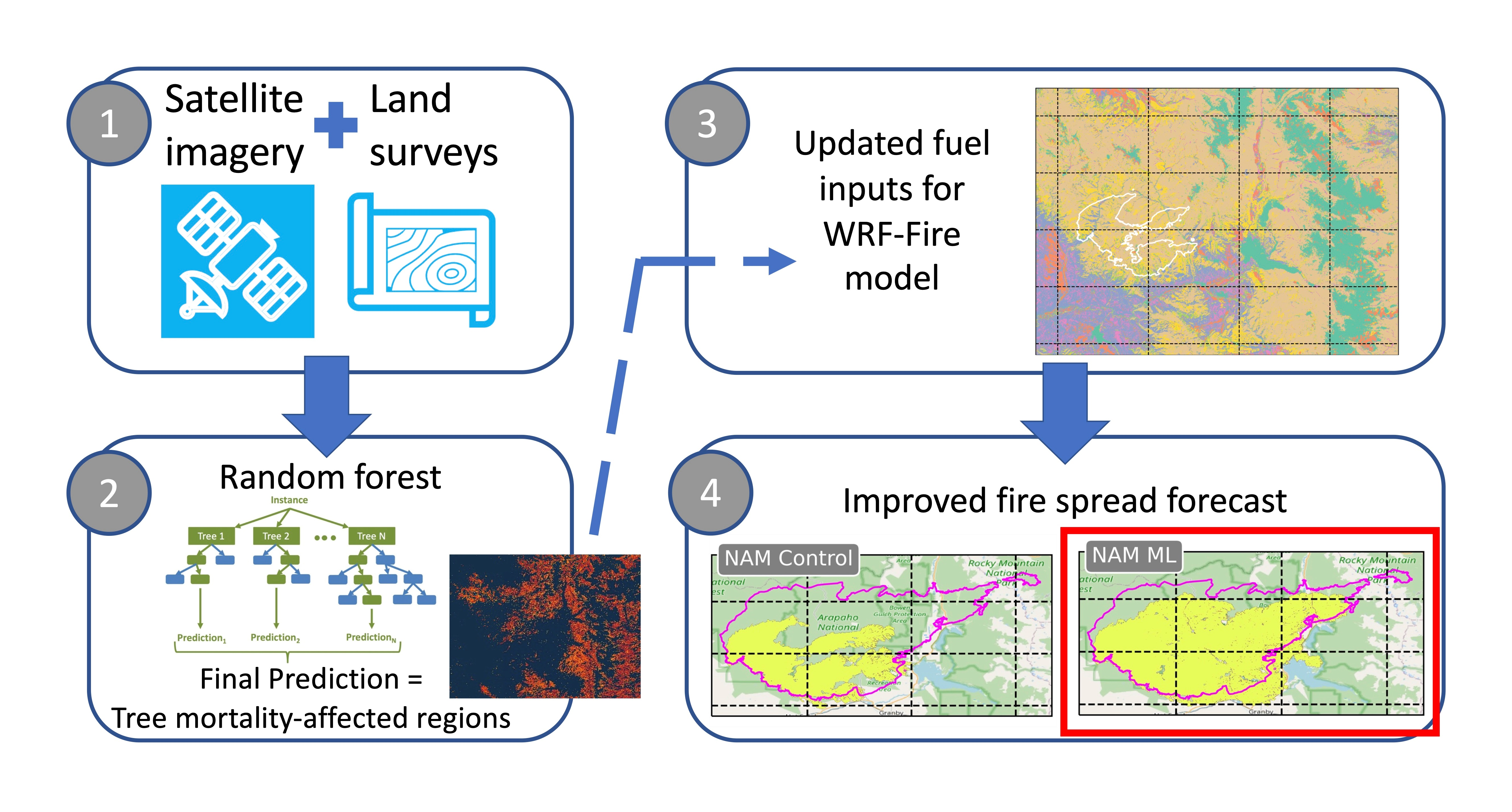
A Computationally Efficient Method for Updating Fuel Inputs for Wildfire Behavior Models Using Sentinel Imagery and Random Forest Classification

 , , , and
Abstract
:
1. Introduction
2. Materials and Methods
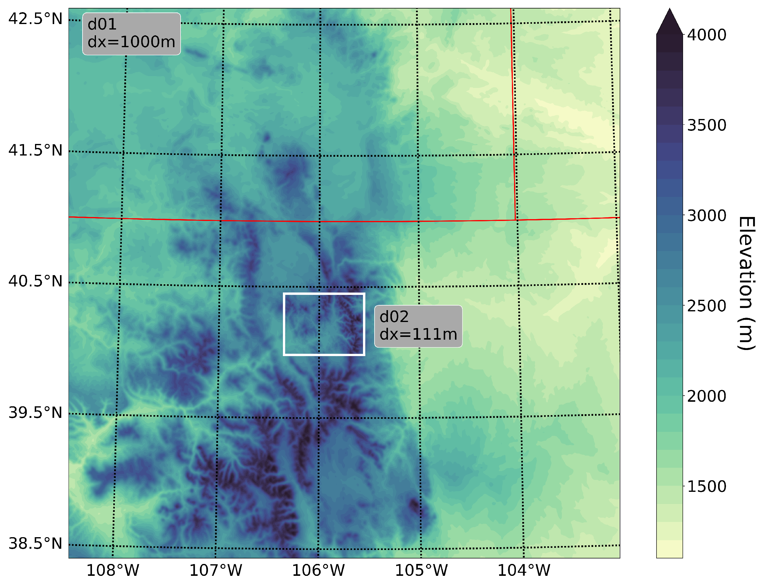
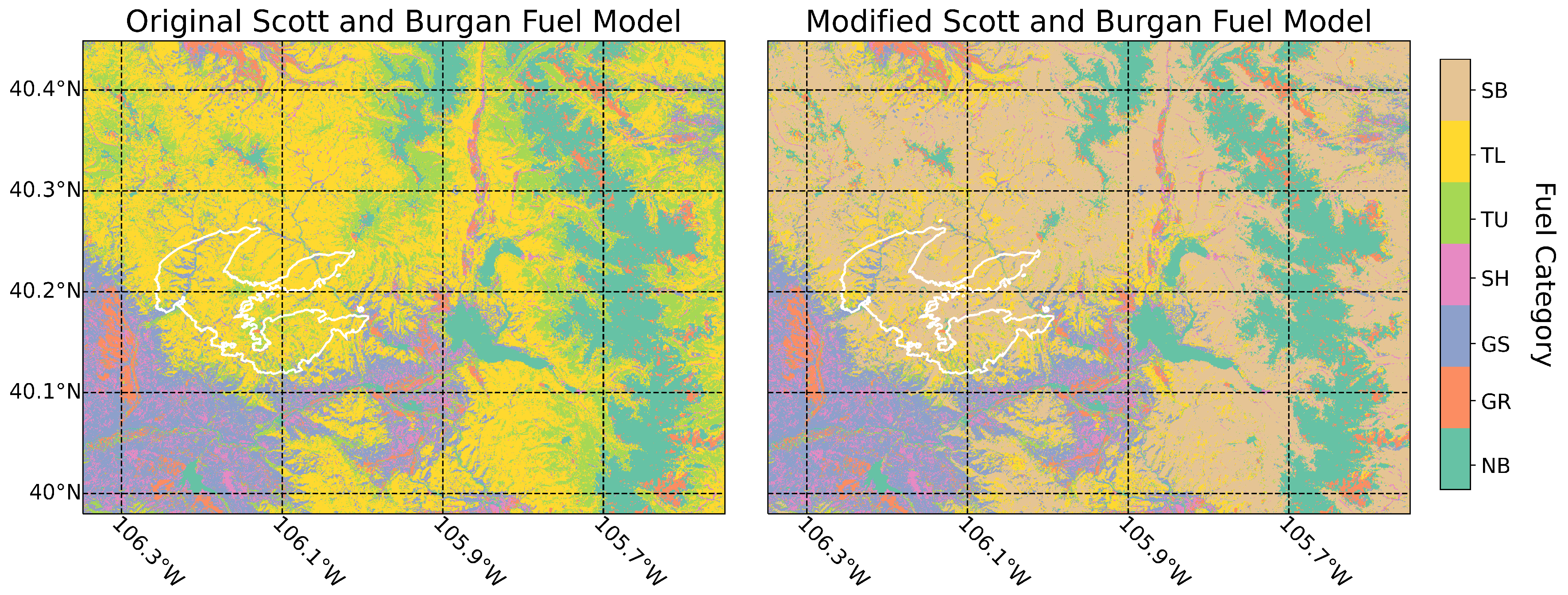
2.1. The East Troublesome Fire Case Study
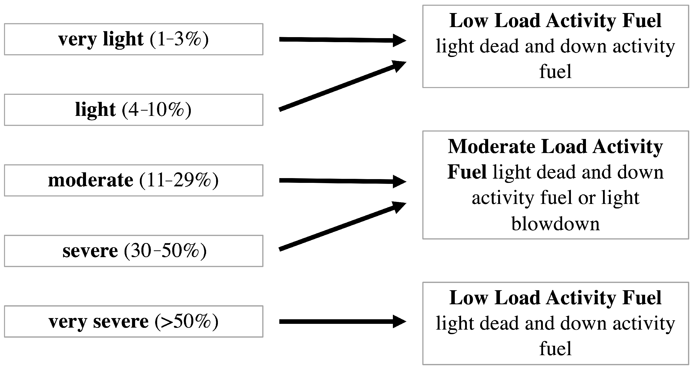
2.2. Machine Learning Approach
2.3. WRF-Fire
3. Results
4. Discussion
5. Conclusions
Author Contributions
Funding
Data Availability Statement
Acknowledgments
Conflicts of Interest
References
- Jain, T.B.; Nelson, A.S.; Bright, B.C.; Byrne, J.C.; Hudak, A.T. Biophysical Settings that Influenced Plantation Survival during the 2015 Wildfires in Northern Rocky Mountain Moist Mixed-Conifer Forests. J. For. 2022, 120, 22–36. [Google Scholar] [CrossRef]
- Radeloff, V.C.; Helmers, D.P.; Kramer, H.A.; Mockrin, M.H.; Alexandre, P.M.; Bar-Massada, A.; Stewart, S.I. Rapid growth of the US wildland-urban interface raises wildfire risk. Proc. Natl. Acad. Sci. USA 2018, 115, 3314–3319. [Google Scholar] [CrossRef] [PubMed] [Green Version]
- Burke, M.; Driscoll, A.; Heft-Neal, S.; Xue, J.; Burney, J.; Wara, M. The changing risk and burden of wildfire in the United States. Proc. Natl. Acad. Sci. USA 2021, 118, 2. [Google Scholar] [CrossRef] [PubMed]
- Parks, S.A.; Abatzoglou, J.T. Warmer and drier fire seasons contribute to increases in area burned at high severity in western US forests from 1985 to 2017. Geophys. Res. Lett. 2020, 47, e2020GL089858. [Google Scholar] [CrossRef]
- Environmental Protection Agency, Climate Change Indicators: Wildfire. Available online: https://www.epa.gov/climate-indicators/climate-change-indicators-wildfires (accessed on 26 January 2022).
- U.S. Department of Agriculture, Biden-Harris Administration Announces Over $1 Billion in Disaster Relief Funds for Post-Wildfire and Hurricane Recovery. Available online: https://www.usda.gov/media/press-releases/2022/01/21/biden-harris-administration-announces-over-1-billion-disaster (accessed on 21 January 2022).
- Cardil, A.; Rodrigues, M.; Ramirez, J.; de-Miguel, S.; Silva, C.A.; Mariani, M.; Ascoli, D. Coupled effects of climate teleconnections on drought, Santa Ana winds and wildfires in southern Cali-fornia. Sci. Total Environ. 2001, 765, 142788. [Google Scholar] [CrossRef] [PubMed]
- Keane, R.E.; Burgan, R.; van Wagtendonk, J. Mapping wildland fuels for fire man-agement across multiple scales: Integrating remote sensing, GIS, and biophysical modeling. Int. J. Wildland Fire 2001, 10, 301–319. [Google Scholar] [CrossRef]
- Rollins, M.G. LANDFIRE: A nationally consistent vegetation, wildland fire, and fuel as-sessment. Int. J. Wildland Fire 2009, 18, 235–249. [Google Scholar] [CrossRef] [Green Version]
- Scott, J.H. Standard Fire Behavior Fuel Models: A Comprehensive Set for Use with Rothermel’s Surface Fire Spread Model; US Department of Agriculture, Forest Service, Rocky Mountain Research Station: Fort Collins, CO, USA, 2005.
- Inciweb, East Troublesome Fire Information. Available online: https://inciweb.nwcg.gov/incident/7242/ (accessed on 1 June 2021).
- Earth Engine Data Catalog, Sentinel-1. Available online: https://developers.google.com/earth-engine/datasets/catalog/COPERNICUS_S1_GRD?hl=en (accessed on 1 June 2021).
- Earth Engine Data Catalog, Sentinel-2. Available online: https://developers.google.com/earth-engine/datasets/catalog/COPERNICUS_S2_SR (accessed on 1 June 2021).
- Earth Engine Data Catalog, USFS Landscape Change Monitoring System v2020.5. Available online: https://developers.google.com/earth-engine/datasets/catalog/USFS_GTAC_LCMS_v2020-5?hl=en (accessed on 1 June 2021).
- U.S. Department of Agriculture, Forest Health. Available online: https://www.fs.fed.us/foresthealth/applied-sciences/mapping-reporting/detection-surveys.shtml (accessed on 10 June 2021).
- Sentinel Online, Sentinel-1. Available online: https://sentinels.copernicus.eu/web/sentinel/user-guides/sentinel-1-sar/applications/land-monitoring (accessed on 13 January 2022).
- Sentinel Online, Sentinel-2. Available online: https://sentinels.copernicus.eu/web/sentinel/user-guides/sentinel-2-msi/applications (accessed on 13 January 2022).
- Breiman, L. Random forests. Mach. Learn. 2001, 45, 5–32. [Google Scholar] [CrossRef] [Green Version]
- Gorelick, N.; Hancher, M.; Dixon, M.; Ilyushchenko, S.; Thau, D.; Moore, R. Google Earth Engine: Planetary-scale geospatial analysis for everyone. Remote Sens. Environ. 2017, 202, 18–27. [Google Scholar] [CrossRef]
- Meddens, A.J.; Hicke, J.A.; Vierling, L.A.; Hudak, A.T. Evaluating methods to detect bark beetle-caused tree mortality using single-date and multi-date Landsat imagery. Remote Sens. Environ. 2013, 132, 49–58. [Google Scholar] [CrossRef]
- Anderson, H.E. Aids to Determining Fuel Models for Estimating Fire Behavior [Grass, Shrub, Timber, and Slash, Photographic Examples, Danger Ratings]; USDA Forest Service General Technical Report; INT-Intermountain Forest and Range Experiment Station (USA): Ogden, UT, USA, 1982. [Google Scholar]
- Krasnow, K.; Schoennagel, T.; Veblen, T.T. Forest fuel mapping and evaluation of LANDFIRE fuel maps in Boulder County, Colorado, USA. For. Ecol. Manag. 2009, 257, 1603–1612. [Google Scholar] [CrossRef]
- Skamarock, W.C.; Klemp, J.B.; Dudhia, J.; Gill, D.O.; Barker, D.M.; Wang, W.; Powers, J.G. A Description of the Advanced Research WRF Version 2; National Center For Atmospheric Research Boulder Co Mesoscale and Microscale Meteorology Div.: Boulder, CO, USA, 2005. [Google Scholar]
- Clark, T.L.; Coen, J.; Latham, D. Description of a coupled atmosphere–fire model. J. Wildland Fire 2004, 13, 49–63. [Google Scholar] [CrossRef] [Green Version]
- Coen, J.L. Modeling Wildland Fires: A Description of the Coupled Atmosphere-Wildland Fire Environment Model (CAWFE); National Center for Atmospheric Research: Boulder, CO, USA, 2013; Volume 38. [Google Scholar]
- Coen, J.L.; Cameron, M.; Michalakes, J.; Patton, E.G.; Riggan, P.J.; Yedinak, K.M. WRF-Fire: Coupled weather–wildland fire modeling with the weather research and forecasting model. J. Appl. Meteorol. Climatol. 2013, 52, 16–38. [Google Scholar] [CrossRef]
- Mandel, J.; Beezley, J.D.; Kochanski, A.K. Coupled atmosphere-wildland fire mod-eling with WRF 3.3 and SFIRE 2011. Geosci. Model. Dev. 2011, 4, 591–610. [Google Scholar] [CrossRef] [Green Version]
- Muñoz-Esparza, D.; Kosović, B.; Jiménez, P.A.; Coen, J.L. An accurate fire-spread algo-rithm in the Weather Research and Forecasting model using the level-set method. J. Adv. Model. Earth Syst. 2018, 10, 908–926. [Google Scholar] [CrossRef] [Green Version]
- Rothermel, R.C. A Mathematical Model for Predicting Fire Spread in Wildland Fuels; Intermountain Forest Range Experiment Station, Forest Service, US Department of Agriculture: Ogden, UT, USA, 1972; Volume 115, pp. 5–32.
- Albini, F.A.; Brown, J.K.; Reinhardt, E.D.; Ottmar, R.D. Calibration of a large fuel burn-out model. Int. J. Wildland Fire 1995, 5, 173–192. [Google Scholar] [CrossRef]
- Nakanishi, M.; Niino, H. An improved Mellor–Yamada level-3 model with con-densation physics: Its design and verification. Bound.-Layer Meteorol. 2004, 112, 1–31. [Google Scholar] [CrossRef]
- McCandless, T.C.; Kosovic, B.; Petzke, W. Enhancing wildfire spread model-ling by building a gridded fuel moisture content product with machine learning. Mach. Learn. Sci. Technol. 2020, 1, 305010. [Google Scholar] [CrossRef]
- Coleman, T.W.; Graves, A.D.; Heath, Z.; Flowers, R.W.; Hanavan, R.P.; Cluck, D.R.; Ryerson, D. Accuracy of aerial detection surveys for mapping insect and disease disturbances in the United States. For. Ecol. Manag. 2018, 430, 321–336. [Google Scholar] [CrossRef]
- Gitelson, A.A.; Keydan, G.P.; Merzlyak, M.N. Three-band model for noninvasive estimation of chlorophyll, carotenoids, and anthocyanin contents in higher plant leaves. Geophys. Res. Lett. 2006, 33. [Google Scholar] [CrossRef] [Green Version]


| Other | Low Load | Moderate Load | High Load | |
|---|---|---|---|---|
| other | 8505 | 337 | 257 | 52 |
| low load | 31 | 256 | 120 | 105 |
| moderate load | 8 | 232 | 457 | 196 |
| high load | 38 | 148 | 179 | 72 |
| Precision | Recall | F1-Score | |
|---|---|---|---|
| other | 0.927 | 0.992 | 0.958 |
| low load | 0.520 | 0.252 | 0.340 |
| moderate load | 0.489 | 0.471 | 0.480 |
| high load | 0.162 | 0.157 | 0.160 |
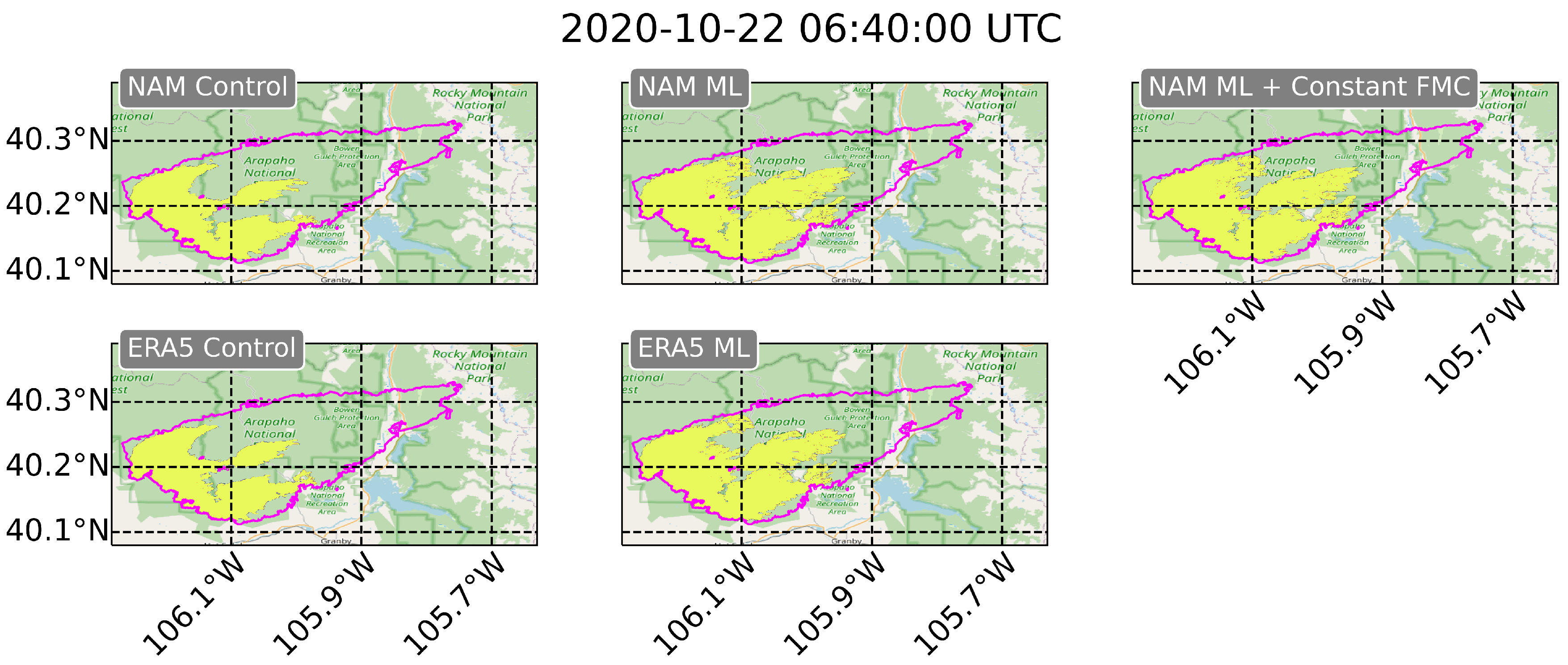
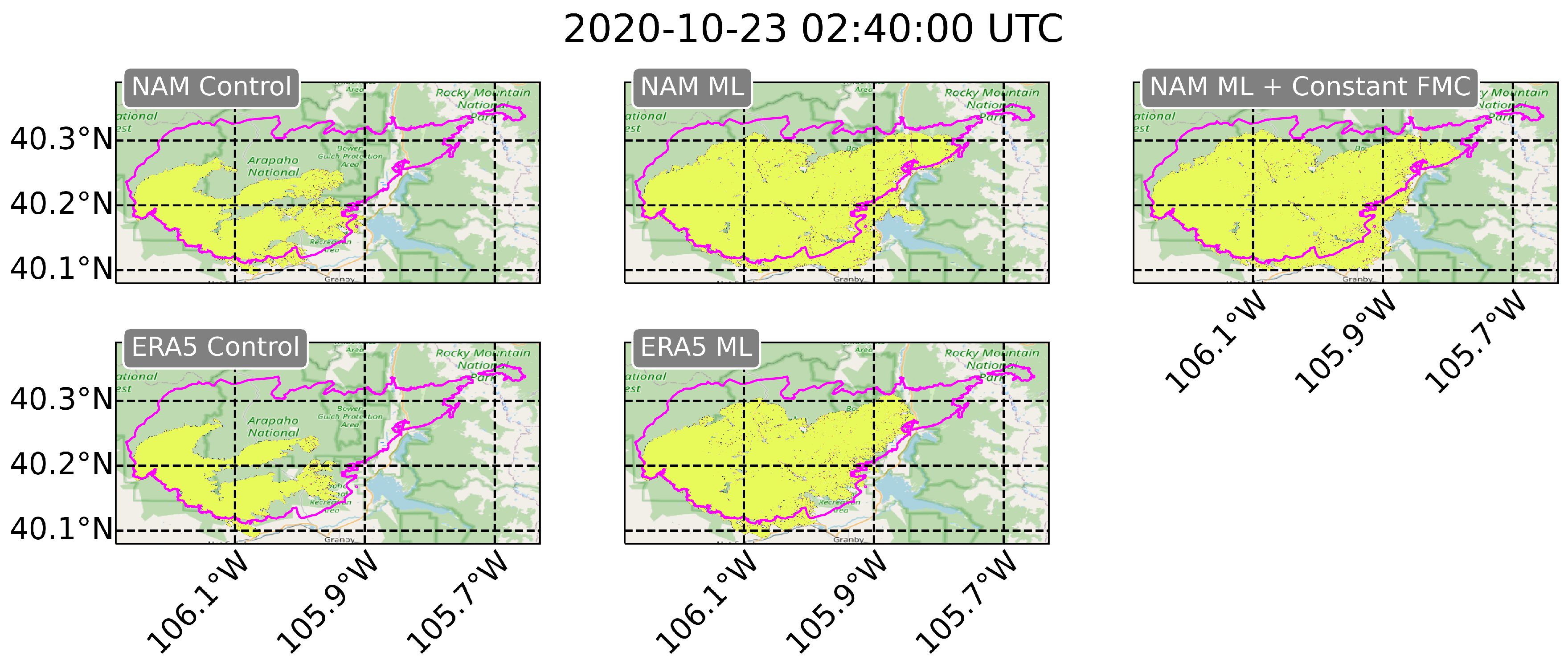
| Date | Simulation | Forecast Area (km2) | Observed Area (km2) | Overlap Area (km2) |
|---|---|---|---|---|
| 10/22/20 0640 UTC | Control | 188.92 | 508.59 | 179.62 |
| Updated Fuels | 285.34 | 508.59 | 258.31 | |
| Updated Fuels + constant FMC | 284.63 | 508.59 | 259.04 | |
| 10/23/20 0240 UTC | Control | 293.87 | 689.57 | 272.17 |
| Updated Fuels | 624.72 | 689.57 | 532.33 | |
| Updated Fuels + constant FMC | 608.39 | 689.57 | 531.15 |
Publisher’s Note: MDPI stays neutral with regard to jurisdictional claims in published maps and institutional affiliations. |
© 2022 by the authors. Licensee MDPI, Basel, Switzerland. This article is an open access article distributed under the terms and conditions of the Creative Commons Attribution (CC BY) license (https://creativecommons.org/licenses/by/4.0/).
Share and Cite
DeCastro, A.L.; Juliano, T.W.; Kosović, B.; Ebrahimian, H.; Balch, J.K. A Computationally Efficient Method for Updating Fuel Inputs for Wildfire Behavior Models Using Sentinel Imagery and Random Forest Classification. Remote Sens. 2022, 14, 1447. https://doi.org/10.3390/rs14061447
DeCastro AL, Juliano TW, Kosović B, Ebrahimian H, Balch JK. A Computationally Efficient Method for Updating Fuel Inputs for Wildfire Behavior Models Using Sentinel Imagery and Random Forest Classification. Remote Sensing. 2022; 14(6):1447. https://doi.org/10.3390/rs14061447
Chicago/Turabian StyleDeCastro, Amy L., Timothy W. Juliano, Branko Kosović, Hamed Ebrahimian, and Jennifer K. Balch. 2022. "A Computationally Efficient Method for Updating Fuel Inputs for Wildfire Behavior Models Using Sentinel Imagery and Random Forest Classification" Remote Sensing 14, no. 6: 1447. https://doi.org/10.3390/rs14061447