Empirical Models for Spatio-Temporal Live Fuel Moisture Content Estimation in Mixed Mediterranean Vegetation Areas Using Sentinel-2 Indices and Meteorological Data

Abstract

Live fuel moisture content (LFMC) is an input factor in fire behavior simulation models highly contributing to fire ignition and propagation. Developing models capable of accurately estimating spatio-temporal changes of LFMC in different forest species is needed for wildfire risk assessment. In this paper, an empirical model based on multivariate linear regression was constructed for the forest cover classified as shrublands in the central part of the Valencian region in the Eastern Mediterranean of Spain in the fire season. A sample of 15 non-monospecific shrubland sites was used to obtain a spatial representation of this type of forest cover in that area. A prediction model was created by combining spectral indices and meteorological variables. This study demonstrates that the Normalized Difference Moisture Index (NDMI) extracted from Sentinel-2 images and meteorological variables (mean surface temperature and mean wind speed) are a promising combination to derive cost-effective LFMC estimation models. The relationships between LFMC and spectral indices for all sites improved after using an additive site-specific index based on satellite information, reaching a R²_adj = 0.70, RMSE = 8.13%, and MAE = 6.33% when predicting the average of LFMC weighted by the canopy cover fraction of each species of all shrub species present in each sampling plot.

1. Introduction

Wildfires are key natural processes shaping ecosystems dynamics. Fire consequences are reduction of soil fertility and damage to forests, land resources, and human assets, but it can also be beneficial, being the source of forest regeneration and nutrient recycling [1]. Some studies suggest that current fire regimes may cause disasters in the sense of inducing abrupt community changes or important soil losses [2], although regions subject to regular fires may have high levels of species richness, and fire may be proposed as a major driver to explaining plant diversity at both community and global scales [3]. However, due to climate and land use change, intense wildfires are becoming more common with an increasing concern of regional and national governments [4,5,6]. Furthermore, wildfires entail ecological and socioeconomic costs, leading fire agencies to invest in developing monitoring tools. Wildfire danger and burnt areas are expected to increase over the century in southern Europe owing to climate warming [7].

Variables affecting wildfire behavior are based on fuel, topography, and weather conditions (wind speed, ambient air temperature, relative humidity), fuel variables being those that describe fuel moisture content and forest structure, such as bulk density and canopy base height. Thus, mathematical models to predict wildland fire behavior on an operational basis take into account spatio-temporal variations of wind speed, fuel moisture, fuel type, and slope [8]. Fuel moisture content (FMC) is a measure of the amount of water in a fuel (vegetation) available to a fire, and it has long been recognized as a major component of fire danger [9]. Sharma et al. [10] quantified the relationships between soil moisture and FMC of mixed live and dead grassland during the growing season in the USA. The FMC of mixed vegetation is categorized as live and dead fuel moisture content. Live fuel moisture content (LFMC) is an essential parameter for operational wildfire risk assessment [11] and forest fire simulations, since it affects vegetation flammability and fire rate of spread [12]. Field based estimations of LFMC are labor and time intensive as well as costly, and they cover small areas. Martin-StPaul et al. [13] described protocols for data collection and confidence interval estimators of LFMC on six different Mediterranean shrub species of 20 sites in Southern France. Yebra et al. [14] presented a global LFMC database for exploring LFMC trends in response to environmental change and LFMC influence on wildfire occurrence, wildfire behavior, and overall vegetation health. Gabriel et al. [15] presented a structured database covering 21 years of LFMC measurements in the Catalan region (Spain). Satellite data-based methods cover large areas; this is why remotely sensed images have been used in numerous studies to obtain LFMC estimations. Yebra et al. [16] reviewed the use of remotely sensed data for estimating LFMC with particular concern towards the operational use of LFMC products for fire risk assessment. Luo et al. [17] showed that LFMC dynamics retrieved from the Moderate Resolution Imaging Spectrometer (MODIS) reflectance product remarkably affect both grassland and forest wildfire occurrence over southwest China. The lower the LFMC is, the more difficult it is to prevent the advance of fire. Reliable and updated estimations of LFMC are needed by fire managers for better decision making [18]. Thus, assessing, improving, and implementing near real-time methods to spatially estimate LFMC is of particular importance [19].

Characterizing variations in LFMC is difficult because both foliar mass and dry mass can change throughout the season [20]. Indeed, meteorological indices are commonly used to predict LFMC across locations [20,21,22,23,24,25]. Martin-StPaul et al. [13] used an LFMC database obtained in the south of France and the island of Corsica during fire seasons from 1996 to 2016 to establish an LFMC linear prediction model by means of a drought index calculated as the ratio between rainfall and evapotranspiration. However, the results were of limited accuracy, as the contrasting water strategies between species mean that the dynamics of LFMC may be different from one species to another in Mediterranean ecosystems. Viegas et al. [21] grouped the species in three sets according to their relatively high, intermediate, or low seasonal variability. In some species, usually classified as anisohydric (e.g., Rosmarinus officinalis), the water content highly varies with climate conditions, whereas in isohydric species (e.g., Pinus halepensis), this is maintained as relatively constant along the whole season [21]. Ruffault et al. [23] achieved good results only over high responsive species (i.e., anisohydric) when using long term meteorological indices. In particular, the leaves of some shrub species show few mechanisms to regulate transpiration, so that their content in LFMC usually shows a strong variation depending on changes in environmental conditions [24]. However, Pellizzaro et al. [25] compared seasonal patterns of LFMC in four species of Mediterranean shrubland using five drought indices based on meteorological variables, showing that meteorological indices might fail when using multiple locations to calibrate models, since they do not account for other environmental factors that might affect water availability, such as soil conditions and species composition that affect water storage and competition, respectively.

LFMC depends on both environmental conditions (liquid water absorption) and species ecophysiology (pigment and structural changes), which impacts spectral reflectance [16]. Remote sensing data take into account the effect of water on the spectral reflectance of vegetation, thus remote sensing approaches consider the influence of plant physiological conditions on the optical properties of vegetation. For instance, Gao and Goetzt [26] showed that radiation absorption in the short-wave infrared was linked to canopy water content, and absorption in the red visible spectrum depended on photosynthetic activity. Indeed, several studies demonstrated the potential use of statistical models to estimate LFMC using vegetation indices from satellite data [27,28,29]. Two main approaches are commonly followed to estimate LFMC from remote sensing data: (1) radiative transfer models (RTM) which are based on physical laws governing relationships between canopy spectra and water content, and (2) empirical models which statistically fit field measures of LFMC with spectral data [16]. The normalized difference vegetation index (NDVI), the enhanced vegetation index (EVI), or the normalized difference water index (NDWI) were used with success in empirical models for this purpose [30,31]. RTMs are robust and easy to generalize (not site specific), but parameterization is complex and depends mostly on model selection. Furthermore, the main difficulty in using RTM for LFMC recovery is the uncertainty of the inversion procedure [32]. Instead, empirical models are simple and easy to calibrate, and they provide a higher level of accuracy than RTM [33]. Moreover, they combine the use of spectral indices with meteorological variables to improve LFMC predictions [28,30,34].

Field based models to estimate LFMC were used in four Mediterranean locations of Catalonia (Spain) [24], in the North Western Sardinia (Italy) [25], and in twenty sites in several regions of Southern France [13,23]. However, most LFMC estimations have relied on satellite products with high temporal resolution but coarse spatial resolution, ranging from 250 m to 1 km (e.g., MODIS, AVHRR, ASTER…) [31,35,36,37,38], whereas developments based on medium spatial resolution images (e.g., from Landsat or Sentinel-1 and 2) are still very scarce [39], suggesting limitations for fragmented forest areas, such as the Mediterranean or many mountainous areas [16]. Since 2015, the European Spatial Agency put at free disposition the new generation of Sentinel-2 sensors which provide data with spatial resolution of 10 m for visible and NIR bands, 20 m for red-edge and SWIR bands, and 60 m for atmospheric bands, thus potentially overcoming coarse resolution limitations. Furthermore, since 2017, the temporal resolution increased to 5 days with the launch of the second Sentinel-2 satellite. Shu et al. [40] demonstrated the potential usage of the Sentinel-2A data for LFMC mapping in 15 field measurements from the USA, South Africa, Australia, and France. More recently, Marino et al. [33] proved that empirical models derived from Sentinel-2 and MODIS data provide similar results in terms of fitting and error level for LFMC estimation in a monospecific shrubland located in Central Spain.

Operational management (e.g., fire risk models) requires predictions for locations where different species coexist. Some considerations emerge when using different locations to fit spatial models of LFMC using remote sensing data. Across locations, different values of vegetation indices for the same LFMC status might be observed due to differences in vegetation cover and optical properties. The same vegetation type can appear significantly different at various stages during intra-annual growth cycles [41]. In addition, variation in optical properties across species due to different chemical composition might generate different spectral patterns for the same LFMC status. Thus, correction factors to adjust the parameters across sites might be required to fit, for instance, a linear model for multiple locations. Previous studies over coarse resolution images followed different approaches to minimize these effects. Chuvieco et al. [30] used land surface temperature retrieved from AVHRR for grassland and shrub species, and they identified an advantage of empirical models in that they can easily include thermal information, which is especially critical in fuels that are more adapted to summer drought, as is the case of most Mediterranean shrubs. Stow and Niphadkar [42] normalized the MODIS vegetation indices using a temporal rescaling based on maximum and minimum values of the time series of each index within each pixel. Peterson et al. [35] used statistics of vegetation indices to improve spatial models calibrating empirical equations that explained site-specific and interannual differences in the amount and the condition of vegetation. To do this, two new independent variables were added to a multiple linear regression analysis: an additive and a multiplicative statistical variable. Caccamo et al. [36] scaled vegetation indices across locations to account for differences in site-specific properties. Finally, in García et al. [43], normalizing the data using the minimum and the maximum in the temporal series improved the results, overcoming the effect of varying vegetation cover and type on the signal recorded by the sensor.

In Spain, the highest average monthly burned area and the highest number of fires in the period 2002–2019 occurred by far from June to October (see https://gwis.jrc.ec.europa.eu/apps/country.profile/charts, last accessed on 14 May 2021). Moreover, in the Valencian region of Spain, the largest burned area occurred in the months of June, July, August, and September (the dry season, see Figure S1 of the supplementary material). This fact, together with the strong climatic differences in the summer season (high temperatures and scarce rainfall) with respect to the rest of seasons, which make difficult the operability of a common LFMC model along the year, point out the need to define a prediction model for LFMC specifically for this period. Moreover, the high fragmentation and the variety of species in Mediterranean ecosystems suggest that the use of high-resolution data can help to capture differences in detailed scales. Shrub communities cover a main part of Mediterranean forests, and they are of particular importance for fire risk monitoring, since ignition and spread are mainly driven by surface and ladder fuels. Usually, different species of shrubs dominate but coexist with other tree species.

Therefore, the present study aimed to build and assess an empirical model of LFMC for mixed vegetation in a Mediterranean area of Spain, combining spectral indices extracted from Sentinel-2 images and meteorological data, based on LFMC field measurements obtained during the dry season when fire risk is higher. Thus, the objectives of this paper were the following: (i) to analyze the seasonal variation of LFMC during the dry season for mixed vegetation in shrub dominated areas of a Mediterranean area of Spain; (ii) to assess the performance of different Sentinel-2 spectral indices on predicting LMFC in pooled locations, accounting also for meteorological information; (iii) to obtain a linear regression model to estimate LFMC during the fire season using Sentinel-2 images and meteorological indices.

This paper is organized as follows. First, study sites and data are described, including field, satellite imagery, and meteorological data. Then, the methodology used to create the LFMC empirical model is presented. Numerical results show the accuracy of our model to obtain an estimation of the weighted LFMC of the shrub species at a fine spatial resolution. In the discussion section, our results are compared with those obtained by other authors, assessing the usefulness of our methodology. The document ends with some conclusions.

2. Materials and Methods

2.1. Study Area

The study area covers a large sector (around 645,000 ha) located in the center of the Valencian region at the east of the Iberian Peninsula. This is an area with a highly variable orography in which the northern part is formed by the NW-SE orientation mountain alignments associated with the Iberian mountain range and the southern part by a set of SW-NE orientation mountain alignments created by the strong tertiary age folds of the Betic mountain range. The central area, remaining in an intermediate domain between these great mountain ranges, is formed by a wide rocky plateau that rises about 800 m above sea level.

Lithologically, in mountainous areas where natural vegetation develops, there is a clear predominance of calcareous rocks, combined in many sectors with marls and clays, which favor the development of shallow basic soils. Locally, at some points, such as near zones A and B (Figure 1), there are some outcrops of siliceous sandstones that generate acid soils. At other points in the study area, we also found gypsum outcrops that, due to their salinity, make local vegetation development difficult. However, the predominance of carbonate spaces and shallow basic soils is very high, and therefore all field samples were taken in these environments.

The study area presents a clear Mediterranean climate with hot summers, mild winters, and poor rainfall (between 350 and 550 mm per year) unevenly distributed throughout the year and the different years. The bulk of rainfall occurs in the autumn months and to a lesser extent in spring and winter. Summer is hot and very dry, which causes a strong water deficit for long periods. Within the study area, however, there are differences associated with (i) altitude (the highest areas are colder in winter and cooler in summer), (ii) distance from the Mediterranean Sea, which creates a system of local breezes that cool the environment and provide moisture to the air, and (iii) local effects caused by the disposition of the relief with respect to the flows of the humid winds. Thus, in the southeastern zone, G-coded points (Figure 1) receive practically twice as much precipitation as the rest of the zones, registering up to 800 mm annually. The entire analyzed area would be framed by thermo and mesomediterranean bioclimatic floors [44].

Although there are significant differences in the vegetation within the studied area, the entire sector remains within the predominance of Pinus halepensis forests and, above all, of different species of shrub, which coexist with the pine trees or replace them. Additionally, in small sectors, there are small groves of Quercus ilex (C, F, and G-coded points in Figure 1). The Pinus halepensis forests are well resistant to drought (it thrives even with annual rainfall of 250 mm), and they adapt to any type of soil, thus this species is clearly dominant in the study area. The area has been widely affected by multiple and recurrent forest fires causing the forest masses to fragment and, currently, the existence of shrubs such as Rosmarinus Officinalis or woody shrubs as Quercus coccifera with small size is common.

A total of 15 plots were selected for model calibration, covering different climatic areas in the province of Valencia, which were grouped into 7 geographic areas coded with letters in Figure 1 and in

Table 1. Description of the calibration plots. The attributes are the following: plot number and zone code (see Figure 1), altitude and slope (in center of the plot), aspect (degrees), the names of the most representative species per plot, and their specific %FCC.

Plot Number	Zone Code	Altitude (m)	Slope (%)	Aspect (Degrees)	Species (% FCC)
1	A	270	15.4	179	Pinus halepensis (35), Rosmarinus Officinalis (25), Quercus coccifera (20), Erica multiflora (20), Pistacia lentiscus (20), Chamaerops humilis (15)
2	A	302	12.5	157	Pinus halepensis (20), Rosmarinus officinalis (30), Quercus coccifera (10), Phillyrea angustifolia (12), Pistacia lentiscus (17), Chamaerops humilis (15)
3	B	217	5.7	127	Pinus halepensis (20), Rosmarinus officinalis (30), Rhamnus lycioides (12), Juniperus oxycedrus (10), Pistacia lentiscus (7)
4	B	203	3.4	90	Pinus halepensis (40), Rosmarinus officinalis (35), Quercus coccifera (5), Juniperus oxycedrus (20), Rhamnus lycioides (10), Erica multiflora (1), Pistacia lentiscus (3), Stipa tenacissima (30)
5	C	957	11.1	353	Pinus halepensis (10), Rosmarinus officinalis (15), Quercus coccifera (40), Juniperus oxycedrus (15), Quercus ilex (35), Juniperus phoenicea (10)
6	D	234	9.8	244	Pinus halepensis (7), Rosmarinus officinalis (30), Quercus coccifera (45), Juniperus oxycedrus (5), Erica multiflora (15)
7	D	267	16.9	76	Pinus halepensis (15), Rosmarinus officinalis (25), Quercus coccifera (35), Cistus albidus (3), Erica multiflora (20)
8	E	548	22.5	112	Pinus halepensis (20), Rosmarinus officinalis (30), Ulex parviflorus (10), Juniperus oxycedrus (15), Quercus coccifera (5), Erica multiflora (30)
9	E	665	15.8	212	Rosmarinus officinalis (50), Quercus coccifera (50), Ulex parviflorus (5), Juniperus oxycedrus (20), Erica multiflora (7)
10	E	672	16.4	345	Pinus halepensis (10), Rosmarinus officinalis (30), Quercus coccifera (50), Juniperus oxycedrus (30), Erica multiflora (7)
11	F	883	3.2	355	Pinus halepensis (5), Rosmarinus officinalis (20), Quercus coccifera (20), Quercus ilex (10), Juniperus oxycedrus (10), Cistus albidus (3)
12	F	873	6.0	73	Quercus ilex (15), Rosmarinus officinalis (10), Quercus coccifera (30), Juniperus oxycedrus (10), Cistus albidus (3)
13	F	882	2.0	45	Rosmarinus officinalis (7), Quercus coccifera (10), Ulex parviflorus (3), Juniperus oxycedrus (20), Quercus ilex (15)
14	G	577	18.8	92	Erica multiflora (10), Quercus coccifera (60), Rosmarinus officinalis (30), Quercus ilex (20), Cistus ladanifer (5)
15	G	390	16.7	0	Erica multiflora (20), Quercus ilex (20), Quercus coccifera (40), Pistacia lentiscus (5), Ulex parviflorus (10)

. Another set consisting of 5 additional plots was considered to validate the models, and its description is shown in

Table 2. Description of the validation plots. The attributes are the following: plot number and zone code (see Figure 1), altitude and slope (in center of the plot), aspect (degrees), the names of the most representative species per plot, and their specific %FCC. Data were collected in the same time period as in calibration plots described in Table 1.

Plot Number	Zone Code	Altitude (m)	Slope (%)	Aspect (Degrees)	%FCC Species
16	A	323	12.4	231	Pinus halepensis (70), Rosmarinus Officinalis (40), Erica multiflora (3), Pistacia lentiscus (30), Phillyrea angustifolia (20)
17	A	299	9.2	150	Pinus halepensis (15), Ulex parviflorus (10), Quercus coccifera (12), Pistacea lentiscus (20), Stipa tenacissima (40), Chamaerops humilis (15)
18	C	740	12.9	36	Pinus halepensis (20), Rosmarinus officinalis (10), Arbutus unedo (20), Juniperus oxycedrus (30), Erica multiflora (15), Ulex parviflorus (10)
19	D	321	29.8	224	Pinus halepensis (70), Rosmarinus officinalis (20), Quercus coccifera (35), Rhamnus lycioides(10), Erica multiflora (20)
20	D	301	5.6	15	Pinus halepensis (80), Rhamnus lycioides (15), Quercus coccifera (40), Pistacia lentiscus (20), Erica multiflora (15)

. All the plots were defined by a central point of a 20 m radius circle, where field samples were collected at different times during the season and a concentric 50 m radius circle with homogeneous vegetation types and density to ensure that corresponding pixels clipped on the satellite images represented the same or very similar areas in the field data collection. Their location was chosen based on the representativeness of the main climatic areas but also on other factors such as the existence of dominant species of Mediterranean shrub, geographical distribution in the study area, easy accessibility, and internal homogeneity of the field plots. Some plots were chosen very close to each other in order to register local variations. Figure 1 (lower left) shows a detail of plots 3 and 4 with their central points and the two concentric circles: one for field data collection (20 m radius) and the other to ensure homogeneity in the clipped samples from satellite images (50 m radius). Table 1 and Table 2 show the dominant species, the altitude, the slope, and the aspect for all sampling plots as codified in Figure 1. The altitudes of sites range from 203 m to 957 m.

Slope and aspect in Table 1 and Table 2 were obtained using a digital terrain model with a resolution of 25 m. Data collection in areas with steep slopes influences solar radiation and thus the LFMC. In general, areas with a low slope were chosen in order to facilitate field sampling. Even if there are some plots with greater slopes where the aspect (orientation) may have some influence in the incoming solar radiation balance, the correlation between solar radiation and field LFMC values was not statistically significant in the fire season.

Moreover, the fraction of canopy cover (%FCC) of each species was visually estimated per plot in the field, as shown in Table 1 and Table 2, to be used for subsequent analyses. Although shrubs dominate in the sampled plots, they coexist with other tree species. However, all the plots belong to a shrub category in which the primary bearer of fire is woody shrubs and shrub litter of high continuity (SH4 category described in document https://agroambient.gva.es/documents/162905929/169203680/Clave+fotográfica+modelos+combustible_20200430/fd5ae58d-3b3f-4e50-866a-d83544a6f1b2, accessed on 12 April 2021). Rosmarinus officinalis is the first dominant shrubland species in several plots, but Quercus coccifera has the highest %FCC in other plots.

2.2. Field Data

Field samples were collected for all species as described in Table 1 and Table 2, transported in sealed bags, fresh weighted, and oven dried in a laboratory to determine fresh and dry weights. Biweekly sampling was performed from June to October 2019. LFMC was estimated as the percentage of water content of vegetation on a dry-weight basis following Equation (1):

$$LFMC=\frac{W_f-W_d}{W_d}\times 100$$

(1)

$W_f$ being the fresh weight and $W_d$ the dry weight. Values of the LFMC obtained per species, plot, and date were calculated, and the representative value of LFMC for each plot was finally assigned as the average LFMC value of the shrub species sampled, weighted according to their %FCC per plot given in Table 1 and Table 2, divided by the sum of the weights of the shrub species. Moving forward, we refer to the weighted average LFMC per as LFMC_WAS (LFMC weighted average in shrubs). Moreover, values of LFMC_WAV (LFMC weighted average in all vegetation species) were also calculated using the weighted average of LFMC with the %FCC from all the vegetation species in the plots. A total of 134 field samples were collected during the sampling period.

2.3. Remote Sensing Data

Spectral indices were calculated using images from Copernicus Sentinel-2 A and B satellites. The multispectral instrument (MSI) on-board Sentinel-2 measures the Earth‘s reflected radiance in thirteen spectral bands with three different spatial resolutions (10 m, 20 m, and 60 m). Sentinel-2 data are freely available, and their parameters provide great convenience in retrieving various vegetation and spectral indices [40]. Moreover, this mission is composed of two satellites allowing for repeated surveys every 5 days. The Level-2A product, i.e., orthorectified and atmospherically corrected to surface reflectance, was accessed via Google Earth Engine using a resampled pixel size of 10 m, independently of the actual resolution of spectral bands. Three types of spectral indices were considered in this study. First were indices more tightly related to vegetation photosynthetic activity containing the red band, which might account for soil and atmospheric corrections, e.g., Enhanced Vegetation Index (EVI), Soil Adjusted Vegetation Index (SAVI), and Optimized Soil Adjusted Vegetation Index (OSAVI) or not, e.g., Normalized Difference Vegetation Index (NDVI), Ratio Vegetation Index (RVI), and Visible Atmospherically Resistant Index (VARI). The second group of spectral indices was related to soil and vegetation water content, since they include short wave infrared (SWIR) bands [45]. Indices in this category were: Normalized Difference Moisture Index (NDMI), Normalized Multi-band Drought Index (NMDI), and Normalized Difference Water Index (NDWI). Their differences were mainly due to the part of the SWIR considered. The third group of indices was related to vegetation greenness, e.g., Vegetation Index-Green (VIGreen) and Transformed Chlorophyll Absorption Index (TCARI), since they contain information on the green band. Moreover, specific leaf area (SLA) index was calculated, which potentially accounts for different leaf types.

Table 3. Spectral indices obtained from Sentinel-2 images and formulas with the band numbers.

Spectral Index	Formulation for Sentinel-2
Enhanced Vegetation Index [46]	EVI = 2.5 × (B8 − B4)/(B8 + 6 × B4 − 7.5 × B2 + 1)
Soil Adjusted Vegetation Index [47]	SAVI = ((B8 − B4)/(B8 + B4 + 0.5)) × 1.5
Optimized Soil Adjusted Vegetation Index [48]	OSAVI = (1 + 0.16) × (B8 − B4)/(B8 + B4 + 0.16)
Normalized Difference Vegetation Index [49]	NDVI = (B8 − B4)/(B8 + B4)
Ratio Vegetation Index [50]	RVI = B8/B4
Visible Atmospherically Resistant Index [51]	VARI = (B3 − B4)/(B3 + B4 − B2)
Normalized Difference Moisture Index [52]	NDMI = (B8 − B11)/(B8 + B11)
Normalized Multi-band Drought Index [53]	-
Normalized Difference Water Index [54]	NDWI = (B8 − B12)/(B8 + B12)
Vegetation Index-Green [55]	VIgreen = (B3 − B5)/(B3 + B5)
Transformed Chlorophyll Absorption Index [56]	TCARI = 3 × ((B5 - B4) − 0.2 × (B5 − B3) * (B5/B4))
Ratio TCARI-OSAVI [56]	TCARI_OSAVI = TCARI/OSAVI
Specific leaf area [57]	SLA = (B9)/(B5 + B12)

shows the formulas for all spectral indices adapted to Sentinel-2 images. The main indices used in the literature for LFMC predictions are highlighted in bold in Table 3.

The values of these indices were calculated for the central pixel of each plot in all dates from the beginning to the end of the LFMC data collection. In addition, to reduce atmospheric noise and residuals from radiometric correction, we used the Savitzky–Golay filter as proposed by [58] for Sentinel-2 NDVI time series implemented in the R package, which uses a third degree polynomial to smooth the time series. This smoothing algorithm avoids oscillations that occur between close dates due to factors other than changes in the humidity of the vegetation (see Figure S2 in supplementary material). Thus, prediction models used the spectral indices described in Table 3 calculated for the central pixel of each plot for every date considered after applying smoothing of the time series. Moreover, windows of 3 × 3 or 9 × 9 pixels were tested and compared (see Appendix B). Values of spectral indices corresponding to the field collection dates were approximated by the smoothed values on the closest Sentinel-2 image acquisition date. Thus, time lag between field dates (reference data collection) and images used for the spectral index calculation was less than 5 days. Furthermore, mean, minimum, maximum, and range values of the time series during the studied period per spectral index were also calculated in each plot to account for specific site effects on surface reflectance in the prediction models.

2.4. Meteorological Data

The Spanish Meteorological Agency (AEMET) registers data of precipitation, temperature, wind, and relative humidity from a set of meteorological stations within our study area. Figure 2 shows their geographical location as a function of the meteorological variable collected together with the location of the field plots. Data of daily precipitation, maximum, minimum, and average daily temperature, average wind speed in km/h for 600 s of the maximum daily wind gusts, and daily maximum and minimum relative humidity were obtained. Values registered at the meteorological observatories were interpolated to LFMC locations using Meteoland R package [59]. This method is similar to the inverse distance weighted but uses a truncated Gaussian filter to select weather stations, including corrections for elevation effects on climatic variables. Relative humidity and wind speed data were also interpolated despite having available a smaller number of stations, since extreme weather conditions such as strong winds can influence the relationships between meteorological data and LFMC values [25].

All meteorological variables were also averaged or accumulated (cumulative values) for the previous days to account for different time windows effects on LFMC. Thus, the average of the daily mean temperatures and the average of the maximum and the minimum daily temperatures were calculated in temporal windows of 7, 15, and 30 days prior to the field data collection date. The cumulative precipitation values for the last 3, 7, 15, 30, and 60 days were also calculated. Other computed indices were the average in the last 3, 7, and 15 days of the daily maximum and minimum relative humidity and average wind speed in Km/h for 600 s of the maximum daily wind gusts.

2.5. Statistical Analysis

The methodology used for this can be summarized in the following steps:

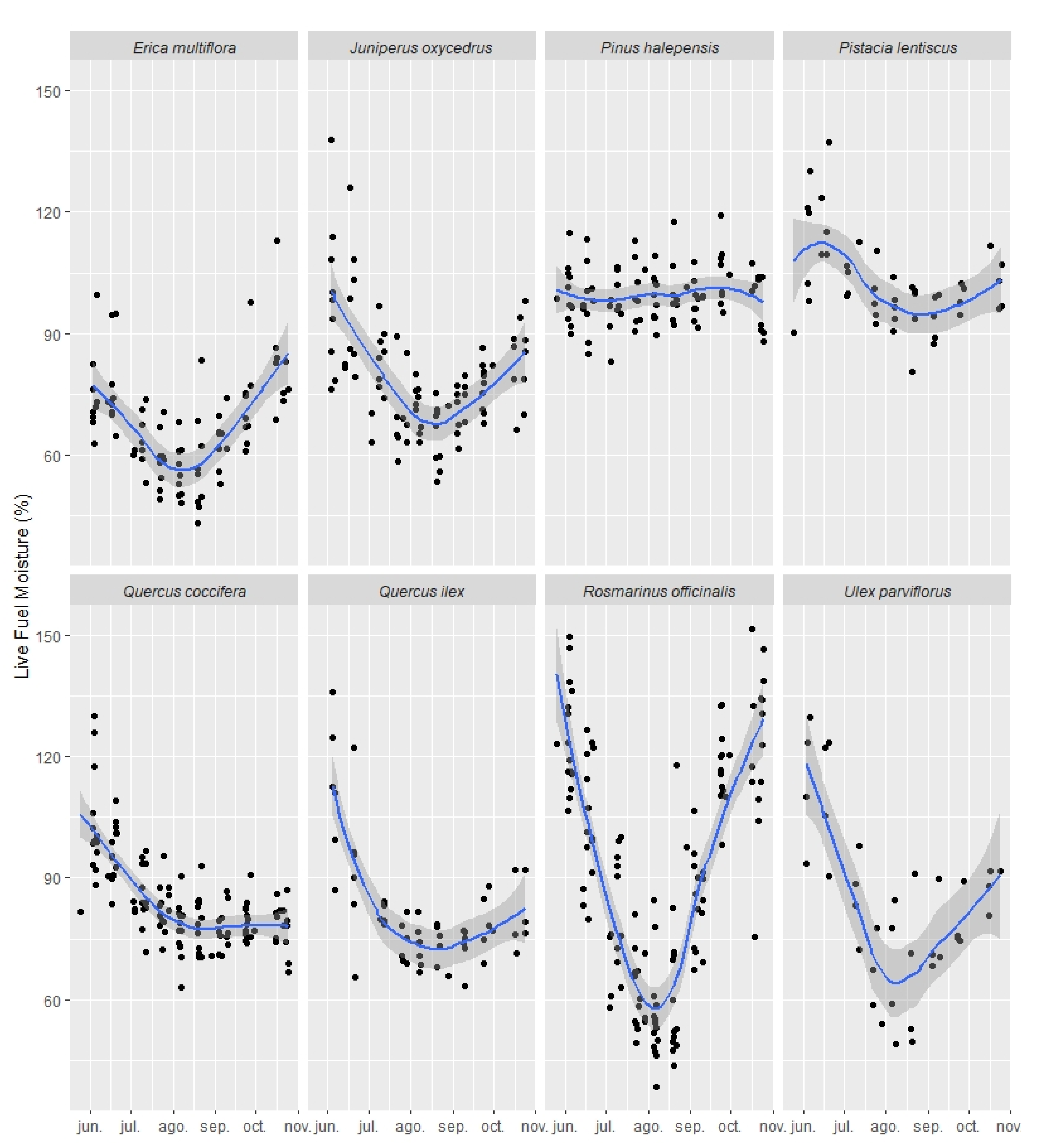
• Analyze the seasonal variation of LFMC across species to assess for different water strategies in the study area.
• Assess the performance of different spectral indices on predicting LMFC_WAS across single locations, accounting also for meteorological information.
• Assess the performance of spectral indices on predicting LMFC_WAS in pooled locations considering site spectral characteristics (e.g., the average of the time series of the selected SI). The inclusion of long-term (cumulative) meteorological data was also evaluated to improve pooled site model predictions.
• Forward stepwise linear regression models were also applied considering all calibration plots from Table 1 distributed in the study area.
• The evaluation of the models was done using 10-fold cross-validation with 3 repetitions and leave-one-site-out cross validation.
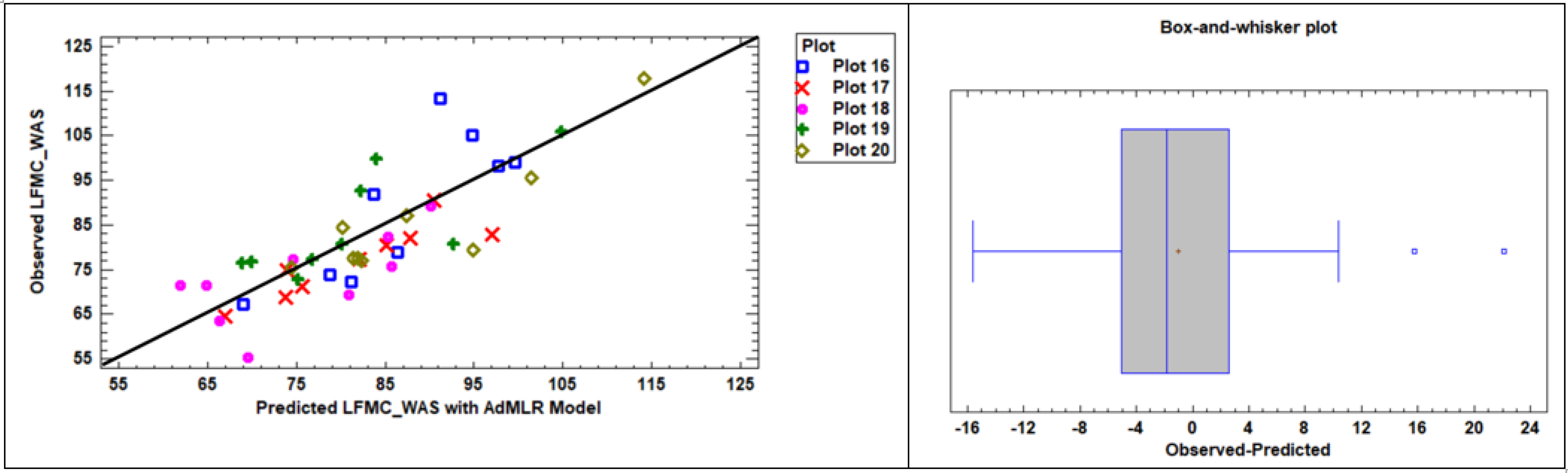
• The precision of the best pooled site regression model was tested in the 5 additional plots of Table 2.
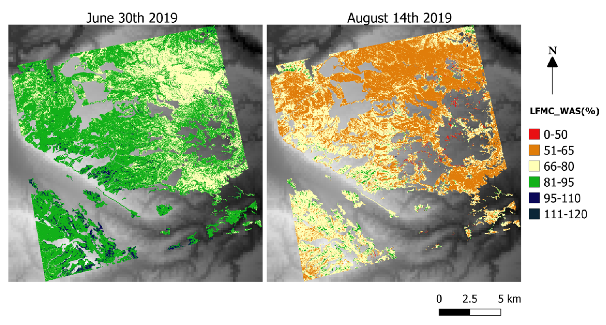
• Final regression model was applied to generate maps of LFMC_WAS estimations using Sentinel-2 images at 10 m/pixel spatial resolution.

Firstly, the temporal evolution of LFMC in different forest species was analyzed as well as LFMC_WAS time series differences in some plots located in the same geographical zone (at short distances, see Figure 1 and Table 1). Fisher’s least significant difference (LSD) procedure [60] was used to identify the plots with the most distant LFMC_WAS mean values, assuming that two mean values were equivalent if their LSD intervals overlapped.

Secondly, correlation between spectral indices (SI) and LFMC_WAS was calculated for each calibration plot, and the SI with the highest R² value was selected. Then, the spectral indices that performed better in a greater number of plots were considered to build a multivariate linear regression model of LFMC_WAS in which the constant and the coefficients varied from one plot to another. Only one spectral index and/or a maximum of two meteorological variables (named Meteo1 and Meteo2) were selected for each site using forward stepwise regression. Thus, initially, we assumed that the adjustment was given by Equation (2):

$$LFMC\_WA{S}_{ij}={\alpha }_j+{\beta }_j{ \mathrm{SI}}_{\mathrm{ij}}+{\delta }_j Meteo{1}_{ij}+{\mu }_j Meteo{2}_{ij}$$

(2)

where subscript “i” refers to the date of data collection and subscript “j” to the plot number. Thus, an equation per plot with different constant and coefficients for the independent variables was obtained.

Thirdly, to account for differences across sites in pooled site regressions, several statistics (average, minimum, maximum, and range) of those SI considered in Equation (2) were calculated for each plot using all available data from Sentinel-2 images from the time period in which a data sample was collected. In this way, these statistics had different values per site but the same in the entire time series. This strategy is similar to the one followed by Peterson et al. [35] aiming to explore if variations between plots in some of these statistics contribute to the prediction of LFMC_WAS. For consistency and robustness, the average of SI at each site was included in pooled site regression models.

Moreover, the inclusion of up to two new meteorological variables was tested, thus combinations with different numbers of independent variables were considered, comparing the adjusted R², the Akaike’s information criterion (AIC), and the Schwarz’s Bayesian information criterion (SBIC) [61] in order to reduce the number of independent variables in the model. This new model would include the SI that performed better in more plots, its seasonal average at each sample point ($\mathrm{Average}\_{\mathrm{SI}}_j$), and two meteorological variables, as expressed by Equation (3):

$$LFMC\_WA{S}_{ij}=\alpha +\gamma \mathrm{Average}\_{\mathrm{SI}}_j+\beta S{\mathrm{I}}_{ij}+\delta Meteo{1}_{ij}+\mu Meteo{2}_{ij}$$

(3)

Model (3) uses the set of LFMC_WAS values obtained in all plots and dates to obtain a common LFMC_WAS model for the study area.

The inclusion of new variables in the model (3) was only justified if their contribution was statistically significant. To avoid multicollinearity, the Pearson’s linear correlation coefficients (R) were calculated between meteorological variables that were candidates to be part of Equation (3). In addition, said coefficient R was also calculated between each meteorological variable and the SI index. Then, meteorological variables having high correlation (R > 0.8) with SI were excluded to avoid imprecise regression coefficients difficult to interpret. In addition, R between Meteo1 and Meteo2 in (3) was smaller than 0.8. High Pearson correlation coefficient between two regressors means probability of multicollinearity. However, a linear relation involves many of the regressors, therefore, it may not be possible to detect such a relationship with a simple pair-wise correlation [62]. Thus, we calculated the variance inflation factor (VIF) for each variable, which was equal to the ratio of the overall model variance to the variance of a model that includes only a single independent variable, informing about the multicollinearity of a model.

The performance of model (3) was compared with the lineal regression model (4):

$$LFMC\_WA{S}_{ij}=\alpha +\beta S{\mathrm{I}}_{ij}+\delta Mete{o}_{ij}$$

(4)

which considers as predictors: SI given in model (3) (without taking into account the additive term of model (3)) with the first meteorological variable that was introduced using forward stepwise linear regression (p-value < 0.05).

Two cross-validation approaches were used to evaluate the models:

(i) Repeated 10-fold cross-validation. The database with plots from Table 1 was randomly divided into 10 groups, and then, alternately, one group was used to validate and the remaining groups were used to calibrate. Cross-validation mean was calculated after repeating the process 3 times in each of the 10 folds.

(ii) Leave-one-site-out cross validation. Once a plot from Table 1 was chosen, the method used all the data except those of that plot to calibrate the model in all dates. Evaluation was done using the adjusted R², RMSE (root mean squared error), and MAE (mean absolute error), repeating the process in all plots.

The performance of the best model selected by cross-validation was evaluated with the five independent sites described in Table 2 in order to get an independent validation.

Finally, that model was applied to generate maps of LFMC_WAS using Sentinel-2 images at 10 m/pixel spatial resolution masking out those areas that did not correspond to shrub or sparse woodland according to the Spanish Forest Map (https://www.miteco.gob.es/es/biodiversidad/servicios/banco-datos-naturaleza/informacion-disponible/mfe50_descargas_ccaa.aspx, accessed on 12 April 2021). Sentinel-2 time series were downloaded and processed using Google Earth Engine to obtain values of NDMI with a temporal resolution of 5 days and the average NDMI at the sample period, which was calculated in each Sentinel-2 pixel. The meteorological data were provided by the Spanish Meteorological Agency (http://www.aemet.es, accessed on 12 April 2021) from stations distributed in the region (see Figure 2) and interpolated to the Sentinel-2 pixel size using the R Meteoland package [59]. Similarly, statistics related to the different temporal scales were calculated for every meteorological variable. Pixels with clouds were filtered out and excluded from maps.

3. Results

3.1. Variation of LFMC across Species and Individual Site Regressions

Different patterns of LFMC behavior were observed along the studied period for different species (Figure 3). Some species, such as Rosmarinus officinalis, presented drastic changes in LFMC (ranging from 38% to 152% from June to October), whereas, in other species, such as Pinus halepensis, changes were very smooth (from 83% to 119%). In general, shrub species such as Rosmarinus officinalis, Ulex parviflorus, Juniperus oxycedrus, and Erica multiflora showed an important LFMC decrease at the beginning of the dry season and a fast recovery after summer. Quercus species also showed an LFMC decrease during summer but with a soft recovery at the end of the dry season. In contrast, Pinus halepensis showed very smooth LFMC variations during the studied period. This behavior is due to the fact that Pinus halepensis tends to have very constant water potential throughout the year [22]. This causes differences between the values of LFMC_WAV and LFMC_WAS due to the fact that two tree species present in our plots, Pinus halepensis and Quercus ilex, were not considered in the calculation of LFMC_WAS. Figure 4, which compares LFMC_WAS values with LFMC_WAV, shows that main differences occurred in the driest period, where the values of LFMC_WAS were lower than those of LFMC_WAV.

The overall trend of LFMC_WAS showed a decrease and recovery at the beginning and the end of the dry season, respectively, and was similar in all the sites, but significant differences were observed between plots located in the same geographical area separated by distances of less than 5 km (e.g., in areas F and G, see Figure S3 of the supplementary material). There was a statistically significant difference of the mean values of LFMC_WAS between several plots according to Fisher’s LSD procedure (Figure 5, e.g., plots 14 and 15, both G-coded in Figure 1).

In order to determine the best spectral index in predicting LFMC_WAS at plot level, per plot regressions were performed for each spectral index, and those with the greatest R² coefficient were selected (second column of

Table 4. R² for several linear regression models using LFMC_WAS as dependent variable. The first column refers to the plot number according to Table 1. The second column shows R² for the best spectral index. The third and the last columns show the R² and the selected variables after applying a forward stepwise regression analysis using NDMI and T60 in column 3 or NDMI, NMDI, T60, T30, and W7 in column 4 (p-value < 0.05). T60 and T30 are the average of daily mean temperatures calculated in 60 and 30 days, respectively, prior to the date of LFMC_WAS collection in the field. W7 is the average of the mean wind speed for 600 s of the maximum daily wind gusts for the previous 7 days.

Plot Number	R2 of LFMC_WAS Model Using the Best Spectral Index		R2 of LFMC_WAS Model Using Forward Stepwise Linear Regression with the Following Predic-Tors: NDMI and T60		R2 of LFMC_WAS Model Using Forward Stepwise Linear Regression with the Following Predictors: NDMI, NMDI, T60, T30, and W7
1	0.56	NDMI	0.56	NDMI	0.56	NDMI
2	0.95	SAVI	0.97	NDMI+T60	0.97	NDMI + T30
3	0.59	EVI	0.46	T60	0.75	T30
4	0.57	NDMI	0.57	NDMI	0.83	T30 + T60
5	0.86	TCARI_OSAVI	0.67	T60	0.67	T60
6	0.77	NMDI	0.64	NDMI	0.92	T30 + W7
7	0.85	NDMI	0.85	NDMI	0.95	T30 + T60
8	0.79	SLA	0.52	NDMI	0.52	NDMI
9	0.77	NMDI	0.94	NDMI + T60	0.96	NMDI + T30
10	0.71	NDMI	0.87	NDMI + T60	0.87	T30
11	0.86	OSAVI	0.78	T60	0.83	T30
12	0.71	NDMI	0.88	T60	0.88	T60
13	0.65	NMDI	0.86	T60	0.95	T60 + W7
14	0.66	NMDI	0.51	NDMI	0.84	NMDI + T30
15	0.66	NMDI	0.77	T60	0.77	T60

). NDMI and NMDI were the best predictors of LFMC_WAS in most of the plots, but the precision of the model varied depending on plot properties. Using NDMI, the best results were obtained in plots 1, 4, 7, 10, and 12, meanwhile, NMDI was the optimal index in plots 6, 9, 13, 14, and 15.

When accounting for climate conditions, the combination of NDMI and T60 (the average of daily mean temperatures calculated in the 60 days prior to the date when LFMC_WAS data were collected) improved the results in plots 2, 9, and 10. On the other hand, temperature is a variable closely related to LFMC_WAS in those plots with a significant presence of Quercus coccifera (plots 5, 6, 7, 10, 11, 12, 13, and 15 according to the last column of Table 1), where spectral indices were not so relevant, and the highest R² values were found using models without NDMI or NMDI. Moreover, the temperature changes explain the lower values of LFMC_WAS in plot 4, in which the species Stipa tenacissima had a high %FCC.

The NDMI and the average of daily mean temperatures in the previous 30 or 60 days were consistent indices for all plots, providing robustness to the results and suggesting high potential to obtain a single prediction model for the area covered by all plots. The average of the mean wind speed for 600 s of the maximum daily wind gusts (W7) for the previous 7 days could improve the accuracy of the model in plots 6 and 13 when used together with the mean temperature in the previous days. Applying forward stepwise linear regression, models with R² greater than 0.46 were obtained in all plots using variables NDMI and/or T60 (column 3 of Table 4).

The value of R² using NDMI as a predictor of LFMC_WAS was always greater than 0.5 with p-values < 0.05, except in three plots (3, 5, and 15), although the coefficients used for the regression models showed high inter-plot variations (see Table S1 in supplementary material). Plot 5 presented the lowest proportion of shrub species, and Quercus ilex species occupied 35% of the %FCC. Plot 15 had different climatic and topographic characteristics, as mentioned is Section 2.1, with higher precipitation in some dates of our study period (see Figure S4 in the supplementary material), making difficult the adjustment even though NDMI values were also higher with respect to other plots.

3.2. Pooled Site Regressions

NDMI was used to build a model to estimate LFMC_WAS combining data from different plots. However, adjusted R² (R²_adj) was equal to 29.07% in the pooled site regression to predict LFMC_WAS using a single spectral index (NDMI) as an explanatory variable, suggesting the need to integrate new complementary variables (see SLR1 (simple linear regression) model in

Table 5. Multiple regression models for LFMC_WAS. The columns represent: formulation, p-value of each coefficient, variance inflation factor (VIF), adjusted R² (R²_adj), root mean square error (RMSE), and mean absolute error (MAE).

Model	Formulation	p-Values	VIF	R2adj	RMSE	MAE
SLR1	$LFMC\_WA{S}_{ij}=81.27+106.879{ \mathrm{NDMI}}_{ij}$	<0.0000		0.29	12.46%	9.93%
		<0.0000	1.0
SLR2	$LFMC\_WA{S}_{ij}=-7.4714+175.578{ \mathrm{NMDI}}_{ij}$	0.6428		0.19	13.26%	10.72%
		<0.0000	1.0
AdLR	$LFMC\_WA{S}_{ij}=81.572-188.442 \mathrm{Average}\_{\mathrm{NDMI}}_j+237.077{ \mathrm{NDMI}}_{ij}$	<0.0000		0.48	10.67%;	8.42%
		<0.0000	3.2329
		<0.0000	3.2329
AdMLR	$LFMC\_WA{S}_{ij}=177.45-79.848 \mathrm{Average}\_{\mathrm{NDMI}}_j+142.125{ \mathrm{NDMI}}_{ij}-2.496 \mathrm{T}{60}_{ij}-4.08 \mathrm{W}{7}_{ij}$	<0.0000		0.70	8.13%	6.33%
		0.0008	4.1737
		<0.0000	4.27214
		<0.0000	1.54064
		<0.0000	1.22462
MLR	$LFMC\_WA{S}_{ij}=154.654+73.676{ \mathrm{NDMI}}_{ij}-2.961 \mathrm{T}{30}_{ij}$	<0.0000		0.66	8.54%;	6.56%
		<0.0000	1.07416
		<0.0000	1.07416

). The use of the NMDI variable as a predictor led to more imprecise results (SLR2 model in Table 5).

In order to modify the constant of the SLR1 model to be adapted to each site, the following predictors were included in the AdLR (linear regression with an additive variable) model: NDMI and average of NDMI computed per plot in the period studied considering interactions between variables. NDMI and Average_NDMI as explanatory variables provided a R²_adj = 0.48 (AdLR model in Table 5), but the interaction of these two variables was not statistically significant, therefore, this term was not included in the model. The use of minimum, maximum, or range of NDMI instead of the average did not improve the adjusted R² value, and their respective products with NDMI were not statistically significant.

Model (3) was tested using NDMI, Average_NDMI, and two meteorological variables as explanatory variables. The best model was obtained using T60 and W7 as meteorological variables (AdMLR (multivariate linear regression with an additive variable) model in Table 5). All variables of AdMLR model were statistically significant, with R²_adj = 0.70, RMSE = 8.13%, and MAE = 6.33%. VIF values were less than five in all the predictors, showing no multicollinearity. Figure 6 shows the evolution of R²_adj according to the number and the type of predictors considered. Using variables NDMI and T60, an R²_adj greater than 0.6 was obtained. Adding W7 R²_adj increased it to 0.67, and by modifying the constant of the model using the Average_NDMI (AdMLR model), an R²_adj of 0.70 was reached.

In model (4), the best results were obtained using NDMI and T30 as independent variables, with the MLR model of Table 5 reaching R²_adj = 0.66, RMSE = 8.54%, and MAE = 6.56%. The variable T30 was the most significant in said model, which only introduced a meteorological variable without taking into account the additive term (Average_NDMI). RMSE and MAE values in MLR and AdMLR models were lower than those obtained in some plots using simple regression between LFMC_WAS and NDMI (Table S1 in the supplementary material).

Figure 7 shows the scatterplot and the fitting line between observed and predicted values for models MLR and AdMLR (coefficients in Table 5). In both models, the slope was close to one and the intercept near zero, suggesting no significant bias in the estimates, and studentized residuals were smaller than three. The greatest differences between the two models occurred at the maximum values of LFMC_WAS (corresponding to the beginning of June and in plots where the wind speed was higher), where the values obtained by the AdMLR model were closer to the field measurements.

The results of MLR and AdMLR models (Table 5) using cross-validation with 10-fold and three repetitions were:

MLR model: R²_adj = 0.71; RMSE = 8.43%; MAE = 6.62%;

AdMLR model: R²_adj = 0.72; RMSE = 8.18%; MAE = 6.61%.

The MLR model obtained reliable results with the leave-one-plot-out cross validation procedure, with R-squared greater than 0.56, RMSE less than 12.5, and MAE less than 11.5 in all plots (

Table A1. RMSE and MAE obtained using leave-one-plot-out cross validation for three regression models. R-squared is the square of Pearson’s correlation coefficient between LFMC_WAS observations and cross validation predictions. The first model used NDMI + T30 as independent variables as in the MLR model of Table 5, the second model used Average_NDMI + NDMI + T60 + W7 as in the AdMLR model of Table 5, and the third model used Average_NDMI + NDMI + T60.

Plot Number	Model with Constant + NDMI + T30			Model with Constant + Average_NDMI + NDMI + T60 + W7			Model with Constant + Average_NDMI + NDMI + T60
Plot	R-Squared	RMSE	MAE	R-Squared	RMSE	MAE	R-Squared	RMSE	MAE
1	0.56	7.48	5.62	0.52	7.67	5.55	0.44	9.08	6.37
2	0.94	3.85	3.23	0.92	4.87	3.84	0.98	3.45	3.07
3	0.85	10.25	8.19	0.81	11	8.86	0.79	11.36	9.36
4	0.76	11.64	9.73	0.66	11.9	10.2	0.70	12.44	10.08
5	0.61	12.72	10.39	0.67	7.35	5.43	0.69	9.87	7.8
6	0.81	6.38	5.33	0.83	6.33	4.86	0.74	8.09	5.85
7	0.94	5.84	5.03	0.90	6.95	6.07	0.90	7.04	5.9
8	0.56	8.35	6.63	0.45	9.31	7.89	0.50	8.59	7.13
9	0.90	6.72	5.5	0.88	5.46	4.43	0.94	5.89	5.37
10	0.92	6.59	5.92	0.86	9.13	7.49	0.86	7.7	6.68
11	0.85	12.45	11.21	0.77	12.4	11.6	0.85	12.82	11.59
12	0.64	12.16	8.37	0.90	8.57	6.58	0.88	10.59	6.52
13	0.81	7.75	5.21	0.92	5	4.37	0.86	6.87	5.57
14	0.69	8.48	7.48	0.58	9.44	7.87	0.58	9.88	8.19
15	0.71	5.38	4.69	0.67	6.46	5.07	0.81	4.68	4.07
Aver.	0.77	8.40	6.83	0.76	8.12	6.67	0.76	8.56	6.90

in Appendix A). The greatest errors occurred in those plots with the lowest or the highest LFMC_WAS values. The AdMLR model improved the predictions at higher altitude plots (zone codes C and F in Table 1) or in zones where the average wind speed calculated by means of W7 was higher (zone code C, see Figure S5 in the supplementary material).

Thus, the selected model for predicting LFMC_WAS was the AdMRL model (Table 5), defined by Equation (5):

$$LFMC\_WA{S}_{ij}=177.45-79.848 \mathrm{Average}\_{\mathrm{NDMI}}_j+142.125 {\mathrm{NDMI}}_{ij}-2.496 \mathrm{T}{60}_{ij}-4.08 \mathrm{W}{7}_{ij}$$

(5)

Model (5) was applied using Sentinel-2 images at 10 m/pixel spatial resolution (SWIR bands were resampled to 10 m resolution for data harmonization) to compute NDMI and the average of the NDMI in our study period in each plot. Meteorological variables (T60 and W7) were interpolated at such spatial resolution.

The precision of model (5) was tested in the five additional plots, which are described in Table 2.

Table 6. Root mean square error (RMSE), mean absolute error (MAE), and the square of Pearson’s correlation coefficient (R-squared) between observed and predicted LFMC_WAS in validation plots given in Table 2. Model (5) was used for prediction of LFMC_WAS.

Plot	R-Squared	RMSE	MAE
16	0.68	9.58%	7.21%
17	0.80	6.07%	4.71%
18	0.46	8.15%	6.85%
19	0.57	8.21%	6.33%
20	0.80	6.42%	4.89%
All	0.65	7.79%	6.00%

shows the values of R-squared, RMSE, and MAE values for those validation plots, which were similar to those obtained for calibration plots. This confirmed the validity of our models in other plots in our study area with a higher presence of non-shrub species in the sample time period.

R-squared was lower in test plot 18, which was in zone C, where the wind speed is higher, and the LFMC_WAS values were also lower (Figure 8). However, it should be mentioned that the wind speed observatories were not optimally located around our sampling points, which could have influenced the accuracy of the results. Errors between observed and predicted LFMC_WAS values followed a normal distribution. Half of the errors were between −5.09 and 2.6, with the mean and the median slightly shifted towards the negative side. The box-and-whisker plot in Figure 8 shows two outliers, which correspond to high values of LFMC_WAS obtained at the end of September in plot 16 and in mid-October in plot 19. These outliers caused the RMSE and the MAE to be slightly higher in these plots.

Figure 9 shows two examples of LFMC_WAS maps obtained using model (5) in an area covered by a Sentinel-2 scene at two different dates, one for 30 June 2019 and the other for 14 August 2019. Figure 9 shows the spatial changes of LFMC_WAS and the temporal changes between two dates during the fire season. The second date corresponds to the month of August, when the lowest values of LFMC were usually reached, in accordance with the values of LFMC_WAS estimated using model (5).

4. Discussion

According to physiological studies [22], species commonly classified as anisohydric highly vary along the dry season, whereas species classified as isohydric tend to maintain relatively constant LFMC. Discriminating water strategies across dominant species might be of particular importance for LFMC monitoring. Fire risk might be higher in areas dominated by anisohydric species since they are more prone to lower the moisture content and thus potentially increase flammability [11]. Higher LFMC variability might result in marked spectral response variations and thus present higher potential to be detected using remote sensing. Previous studies showed that LFMC of shrublands can be retrieved with higher accuracy than LFMC of grasslands and woodlands [16]. However, it is necessary to improve the accuracy of LFMC estimates of shrublands in heterogeneous canopies using empirical LFMC models fitted in the fire season [18].

Results of this paper suggest that different water strategies influence LFMC estimations obtained from remote sensing data. For instance, contrasting LFMC trends across co-occurring species (e.g., Pinus halepensis and Rosmarinus officinalis) within a 10 m pixel area might lead to slight LFMC variations due to averaging values, making difficult estimations and interpretation for risk management. Recently, LFMC models in monospecific shrub areas of Spain were explored using indices derived from Sentinel-2 images [33,63]. However, in most of the forest areas of Spain, different shrub species are frequently mixed [28,30], as in our study area. Therefore, the information obtained through the variables extracted from satellite images is influenced by the species proportion within each pixel. Thus, the integration of LFMC measures across co-occurring species into a unique value with an ecological/physical meaning is not straightforward. In this paper, a weighted average using the cover fraction of shrub species was considered to minimize this effect. However, it is important to notice that LFMC, here expressed as the percentage of water content of vegetation on a dry-weight basis, does not account for absolute differences on water content across species captured by the satellite sensor [20] or for differences on dry matter content [64].

Our results showed the potential use of near-real-time remote sensing data from Sentinel-2 for spatially monitoring LFMC estimations of shrublands at fine scales during the fire season. Accounting for site-specific spectral characteristics and long-term weather conditions allowed us to build a spatial model based on multiple locations to project not only over monospecific but also over heterogeneous areas, which might substantially improve wildfire risk monitoring. Model performance for each single location was mostly within the range of previous studies [30,33,34,37,63]. Most of them included both wet and dry seasons, whereas our study was only focused on the latter. Focusing on the dry season ensures that our model is calibrated to predict LFMC when fire risk is higher rather than to detect LFMC variations across seasons, which can be less useful for operational management. However, models in this study should be considered with caution in operational management, as they are fitted only with data from one summer season. Moreover, site-specific spectral characteristics accounted for in Average_NDMI included values from a limited number of plots that might not be able to capture the high variability of spectral response of heterogeneous vegetation commonly found in Mediterranean regions. Hence, results regarding model performance may vary significantly when applied to predict LFMC values under different weather or site conditions. It will be also useful to obtain models enabling prediction of the changes between seasons that are also important for operational fire management (e.g., fire hazard monitoring and prevention planning) in order to better predict the potential changes of vegetation moisture from low flammability to moderate and high flammability levels. This could be especially relevant under climate change scenarios currently affecting our study area as well as other Mediterranean regions.

Although theory suggests that water indices might perform better [45], contrasting results across different studies [16] suggest that confounding factors such as species traits and surrounding conditions might affect the performance of different remote sensing indices. Disentangling factors affecting the performance of different indices across environmental conditions might be useful for LFMC monitoring. Chuvieco et al. [30] already mentioned that LFMC values in most Mediterranean shrubs cannot be accurately estimated using only NDVI values, because chlorophyll and LAI changes caused by LFMC variations are less apparent in shrub species than in grasslands. In this paper, spectral indices related to moisture content, calculated using Sentinel-2 images, were explored (e.g., NDMI) in order to provide LFMC estimations of shrublands. Using these indices, better results were obtained than with those related to photosynthesis activity (e.g., NDVI, VARI, EVI) and greenness (e.g., VIgreen), because, in some plots of our study area, the rise in moisture content in September was not necessarily accompanied by an increase in photosynthetic activity or leaf area. Recall that the EVI index from MODIS data was used in some references, such as [18,34]. Marino et al. [63] used VARI, EVI, and VIgreen indices extracted from Sentinel-2 images. Moreover, Marino et al. [33] calculated empirical models with Sentinel-2 images using VARI and SAVI. However, results of this paper proved that the properties of moisture indices can help to better estimate LFMC in our study area in the fire season.

Coefficients of the regression models of LFMC using SI as predictors change across locations, suggesting that a model fitted with data from multiple locations should include additional variables to improve accuracy. When including the seasonal average of NDMI of each location, a substantial model improvement is found, since it allows to consider site-specific spectral characteristics that affect the variation rate of NDMI. For instance, differences in vegetation cover, aspect, or soil water retention might affect these responses. Indeed, Peterson et al. [35] found that using statistics of spectral indices increases model performance. They suggested that this approach was more flexible than scaling/normalization across site approach [36,42] because the former might influence the slope or the intercept of regression lines. Our results also showed that the inclusion of meteorological variables potentially improves the model performance in the fire season in a mixed Mediterranean vegetation area. Previous studies also showed the potential synergic effect of these variables [30,34]. In our area and year studied, variables of precipitation and relative humidity were less related to LFMC than the average temperature (see Table S2 of the supplementary material). For example, precipitation and relative humidity slightly increased the value of R²_adj and decreased the values of RMSE and MAE when introduced into the MLR model (Table S3 of the supplementary material). Among the precipitation variables, the accumulated precipitation in the last 60 days (P60) was the one that presented a greater correlation with LFMC_WAS (Table S2). However, this correlation depended on location, being higher in zones A, B, C, D, and E given in Figure 1 and lower in zones F and G (Figure S4 in supplementary material), thus P60 was not chosen by our variable selection procedure in the final model (5). This suggests that precipitation is an important variable, but its influence is more sensitive to variations than temperature, and it should always be considered as a cumulative factor over a period of time. This behavior could change depending on the seasons, thus inter-seasonal analysis should be carried out to analyze these variables in atypical climate seasons. In addition, Table A1 (Appendix A) shows that there were only a few plots where LFMC_WAS values could be predicted with minimum RMSE and MAE without considering variable W7 in the AdMLR model.

Our final model (AdMLR model (5)) performed within the range of previous studies which accounted for multiple locations [35,43] despite being built with LFMC measurements from a variety of species with different behavior related to water variations, although our study period was limited to one summer season. The relationships between LFMC and the SIs for all sites improved in [43] after using their relative values and relative LFMC, increasing R² from 0.19 up to 0.48 for relative EVI. This increase is similar to that showed in our models SLR1, SLR2, and AdLR described in Table 5 of this paper. The best model described in [35] with two independent variables for the pooled analyses used VARI and the median of VIgreen for chaparral with an average cross-validated and adjusted R² of 0.712, which is similar to that of our final model (AdMLR model of Table 5). In order to reproduce our method using a series of several years, statistics considering different values per site and per year should be introduced to address inter-annual and inter-site differences in meteorological conditions and vegetation response. Chuvieco et al. [30] predicted LFMC values of grasslands and Cistus ladanifer in a study area of Spain using NDVI, surface temperature, and a function of the day of the year. Later, Garcia et al. [28] revised the methodology to avoid high over-estimation of LFMC values when applied to dry years using a drought index to discriminate between dry and wet years at the beginning of the spring season with R² = 0.71 for shrubs. As future work, we envisage the validation of our model in a series of years with different precipitation regimes.

Equation (5) was applied using predictors calculated at 10 m/pixel spatial resolution. Averaging spectral indices in 3 × 3 pixel windows, the accuracy of the model slightly improved, but using 9 × 9 pixel windows resulted in slightly lower accuracy values (see

Table A2. Multiple regression models for LFMC_WAS with two spatial resolutions of predictors. The columns represent: spatial resolution of predictors, formulation, p-values of each coefficient, adjusted R² (R²_adj), root mean square error (RMSE), and mean absolute error (MAE).

Spatial Resolution of Predictors	Formulation	p-Values	R2adj	RMSE	MAE
3 × 3 Sentinel-2 pixels	$LFMC\_WA{S}_{ij}=178.174-97.495 \mathrm{Average}\_{\mathrm{NDMI}}_j+159.328 {\mathrm{NDMI}}_{ij}-2.466 \mathrm{T}{60}_{ij}-4.23 \mathrm{W}{7}_{ij}$	<0.0000, <0.0000, <0.0000, <0.0000 <0.0000	0.72	7.80%	5.95%
9 × 9 Sentinel-2 pixels	$LFMC\_WA{S}_{ij}=180.43-143.746 \mathrm{Average}\_{\mathrm{NDMI}}_j+177.789 {\mathrm{NDMI}}_{ij}-2.433 \mathrm{T}{60}_{ij}-4.497 \mathrm{W}{7}_{ij}$	<0.0000, <0.0000 <0.0000, <0.0000, <0.0000	0.68	8.33%	6.55%

in Appendix B). Comparing these models of Table A2 with the statistics from Table 5, the main difference was found in the coefficient that multiplied the temporal average of NDMI ($\mathrm{Average}\_{\mathrm{NDMI}}_j$).

AdMLR model (5) was fitted to predict LFMC calculated as weighted average of only the shrub species sampled in shrub areas. However, plots used for calibration of that model had up to 40% tree cover. Prediction models using the weighted average of LFMC from all the vegetation species in the plots were also tested, reaching a slightly smaller R²_adj but also smaller RMSE and MAE, as shown in Table S4 in the supplementary material. The R-square between observed and predicted values decreased when applying the equivalent of model (5) for LFMC_WAV (second row of Table S4) to the validation plots described in Table 2 (R² = 0.48). This was due to the different behavior of Pinus halepensis species (Figure 3) with respect to shrub species. Although all plots were classified as shrub, in some plots of the validation data, the FCC of Pinus halepensis was higher than 40%, which is the maximum FCC reached in the calibration data.

5. Conclusions

This paper described the construction of empirical models to estimate LFMC_WAS using data obtained from 15 plots in a Mediterranean area of Spain during the fire season of 2019 (1 June to 31 October), where different forest species coexist, and the area is dominated by shrubs. In our study area, there were changes in the LFMC_WAS time series caused by environmental factors together with other spatial changes, thus LFMC_WAS values differed significantly in the different plots studied. Empirical models for LFMC_WAS considered several spectral indices extracted from Sentinel-2 satellite images along with variables obtained by interpolating meteorological data. Our final model (Equation (5) and AdMLR model in Table 5) for predicting LFMC_WAS in each Sentinel-2 pixel used values of NDMI calculated in each time value, but with the average of the NDMI in the whole period analyzed and two meteorological variables. Mean temperature of the previous 60 days was the best meteorological variable, improving the model accuracy while avoiding multicollinearity. The average wind speed in the previous 7 days for 600 s of the maximum daily wind gusts allowed modeling small local changes caused by wind.

Results obtained in this paper showed that different spectral indices—and particularly the NDMI—allow detecting changes of LFMC_WAS at temporal and spatial levels. Joining the information on spectral indices together with meteorological variables contributed to reduce the errors inherent to the model. The fitted model was built to take into account the spatial and the temporal variability of LFMC_WAS at the Sentinel-2 pixel resolution level. Thus, LFMC_WAS was estimated by means of the NDMI (extracted at pixel level from Sentinel-2 satellite images) and the meteorological variables (temperature and wind speed interpolated to 10 m pixel size) plus a constant that modeled spatial differences (site-specific) during the fire season, obtaining R²_adj = 0.70, RMSE = 8.13%, and MAE = 6.33%.

Overall variations of LFMC_WAS in our study area are mainly seasonal. In this sense, the cumulative mean temperature is sensitive to seasonal cycles, thus the proposed model is adapted to seasonal changes in LFMC but could have limitations in atypical years with abrupt changes of LFMC (e.g., due to summer storms). Therefore, the model needs to be tested in the future using a series of years with a wider range of meteorological conditions to analyze the effect of anomalous intense precipitation including the summer. In this case, a cumulative precipitation variable could be introduced as a predictor in the model.

In summary, the work carried out showed the possibility of estimating LFMC_WAS in almost real time based on Sentinel 2 images and available meteorological data. LFMC_WAS maps were generated for two dates as a preliminary product that, after tunning the model by including a larger spatio-temporal data set, could be used in the near future in an operational basis.

References

1. Dimitriou, A.; Mantakas, G.; Kouvelis, S. An Analysis of Key Issues that Underlie Forest Fires and Shape Subsequent Fire Management Strategies in 12 Countries in the Mediterranean Basin; Final report prepared by Alcyon for WWF Mediterranean Programme Office and IUCN. 2001. Available online: https://ec.europa.eu/environment/forests/pdf/meeting140504_wwfsecondocument.pdf (accessed on 31 August 2021).
2. Pausas, J.G.; Llovet, J.; Rodrigo, A.; Vallejo, V.R. Are wildfires a disaster in the Mediterranean basin?—A review. Int. J. Wildland Fire 2008, 17, 713–723. [Google Scholar] [CrossRef]
3. He, T.; Lamont, B.B.; Pausas, J.G. Fire as a key driver of Earth’s biodiversity. Biol. Rev. 2019, 94, 1983–2010. [Google Scholar] [CrossRef]
4. Tedim, F.; Leone, V.; Amraoui, M.; Bouillon, C.; Coughlan, M.R.; Delogu, G.M.; Fernandes, P.M.; Ferreira, C.; McCaffrey, S.; McGee, T.K.; et al. Defining Extreme Wildfire Events: Difficulties, Challenges, and Impacts. Fire 2018, 1, 9. [Google Scholar] [CrossRef] [Green Version]
5. San-Miguel-Ayanz, J.; Durrant, T.H.; Boca, R.; Liberta, G.; Branco, A.; de Rigo, G.; Ferrari, D.; Maianti, P.; Vivancos, T.; Oom, D.; et al. Forest Fires in Europe, Middle East and North Africa 2018; Technical Report EUR 29856 EN; Publications Office of the European Union: Luxembourg, 2019; ISBN 978-92-76-12591-4. [Google Scholar] [CrossRef]
6. Ribeiro, L.; Viegas, D.; Almeida, M.; McGee, T.K.; Pereira, M.G.; Parente, J.; Xanthopoulos, G.; Leone, V.; Delogu, G.M.; Hardin, H. Extreme wildfires and disasters around the world. In Extreme Wildfire Events and Disasters, Root Causes and New Management Strategies; Elsevier: Amsterdam, The Netherlands, 2020; pp. 31–51. [Google Scholar] [CrossRef]
7. Dupuy, J.-L.; Fargeon, H.; Martin-StPaul, N.; Pimont, F.; Ruffault, J.; Guijarro, M.; Hernando, C.; Madrigal, J.; Fernandes, P. Climate change impact on future wildfire danger and activity in southern Europe: A review. Ann. For. Sci. 2020, 77, 1–24. [Google Scholar] [CrossRef]
8. Cruz, M.G.; Alexander, M.E. The 10% wind speed rule of thumb for estimating a wildfire’s forward rate of spread in forests and shrublands. Ann. For. Sci. 2019, 76, 44. [Google Scholar] [CrossRef] [Green Version]
9. Brown, A.A.; Davis, K.P. Fire Danger Rating. In Forest Fire: Control and Use, 2nd ed.; Mac Graw Hill: New York, NY, USA, 1973; pp. 217–259. [Google Scholar]
10. Sharma, S.; Carlson, J.D.; Krueger, E.S.; Engle, D.M.; Twidwell, D.; Fuhlendorf, S.D.; Patrignani, A.; Feng, L.; Ochsner, T.E. Soil moisture as an indicator of growing-season herbaceous fuel moisture and curing rate in grasslands. Int. J. Wildland Fire 2021, 30, 57–69. [Google Scholar] [CrossRef]
11. Chuvieco, E.; Aguado, I.; Yebra, M.; Nieto, H.; Salas, J.; Martin, M.P.; Vilar, L.; Martínez, J.; Martín, S.; Ibarra, P.; et al. Development of a framework for fire risk assessment using remote sensing and geographic information system technologies. Ecol. Model. 2010, 221, 46–58. [Google Scholar] [CrossRef]
12. Fares, S.; Bajocco, S.; Salvati, L.; Camarretta, N.; Dupuy, J.-L.; Xanthopoulos, G.; Guijarro, M.; Madrigal, J.; Hernando, C.; Corona, P. Characterizing potential wildland fire fuel in live vegetation in the Mediterranean region. Ann. For. Sci. 2017, 74, 1. [Google Scholar] [CrossRef] [Green Version]
13. Martin-StPaul, N.; Pimont, F.; Dupuy, J.L.; Rigolot, E.; Ruffault, J.; Fargeon, H.; Cabane, E.; Duché, Y.; Savazzi, R.; Toutchkov, M. Live fuel moisture content (LFMC) time series for multiple sites and species in the French Mediterranean area since 1996. Ann. For. Sci. 2018, 75, 57. [Google Scholar] [CrossRef] [Green Version]
14. Yebra, M.; Scortechini, G.; Badi, A.; Beget, M.E.; Boer, M.M.; Bradstock, R.; Chuvieco, E.; Danson, F.M.; Dennison, P.; De Dios, V.R.; et al. Globe-LFMC, a global plant water status database for vegetation ecophysiology and wildfire applications. Sci. Data 2019, 6, 155. [Google Scholar] [CrossRef] [Green Version]
15. Gabriel, E.; Delgado-Dávila, R.; De Cáceres, M.; Casals, P.; Tudela, A.; Castro, X. Live fuel moisture content time series in Catalonia since 1998. Ann. For. Sci. 2021, 78, 1–10. [Google Scholar] [CrossRef]
16. Yebra, M.; Dennison, P.; Chuvieco, E.; Riano, D.; Zylstra, P.; Hunt, E.R.; Danson, F.; Qi, Y.; Jurdao, S. A global review of remote sensing of live fuel moisture content for fire danger assessment: Moving towards operational products. Remote Sens. Environ. 2013, 136, 455–468. [Google Scholar] [CrossRef]
17. Luo, K.; Quan, X.; He, B.; Yebra, M. Effects of Live Fuel Moisture Content on Wildfire Occurrence in Fire-Prone Regions over Southwest China. Forests 2019, 10, 887. [Google Scholar] [CrossRef] [Green Version]
18. Arganaraz, J.P.; Landi, M.A.; Bravo, S.J.; Gavier-Pizarro, G.I.; Scavuzzo, C.M.; Bellis, L.M. Estimation of Live Fuel Moisture Content From MODIS Images for Fire Danger Assessment in Southern Gran Chaco. IEEE J. Sel. Top. Appl. Earth Obs. Remote Sens. 2016, 9, 5339–5349. [Google Scholar] [CrossRef]
19. Bowman, D.; Williamson, G.; Yebra, M.; Lizundia-Loiola, J.; Pettinari, M.L.; Shah, S.; Bradstock, R.; Chuvieco, E. Wildfires: Australia needs national monitoring agency. Nature 2020, 584, 188–191. [Google Scholar] [CrossRef]
20. Jolly, W.M.; Hadlow, A.M.; Huguet, K. De-coupling seasonal changes in water content and dry matter to predict live conifer foliar moisture content. Int. J. Wildland Fire 2014, 23, 480–489. [Google Scholar] [CrossRef] [Green Version]
21. Viegas, D.; Pinol, J.; Viegas, M.T.; OgayaD, R. Estimating live fine fuels moisture content using meteorologically-based indices. Int. J. Wildland Fire 2001, 10, 223. [Google Scholar] [CrossRef]
22. Helman, D.; Lensky, I.M.; Tessler, N.; Osem, Y. A Phenology-Based Method for Monitoring Woody and Herbaceous Vegetation in Mediterranean Forests from NDVI Time Series. Remote Sens. 2015, 7, 12314–12335. [Google Scholar] [CrossRef] [Green Version]
23. Ruffault, J.; Martin-StPaul, N.; Pimont, F.; Dupuy, J.-L. How well do meteorological drought indices predict live fuel moisture content (LFMC)? An assessment for wildfire research and operations in Mediterranean ecosystems. Agric. For. Meteorol. 2018, 262, 391–401. [Google Scholar] [CrossRef]
24. Castro, F.; Tudela, A.; Sebastià, M.T. Modeling moisture content in shrubs to predict fire risk in Catalonia (Spain). Agric. For. Meteorol. 2003, 116, 49–59. [Google Scholar] [CrossRef]
25. Pellizzaro, G.; Cesaraccio, C.; Duce, P.; Ventura, A.; Zara, P. Relationships between seasonal patterns of live fuel moisture and meteorological drought indices for Mediterranean shrubland species. Int. J. Wildland Fire 2007, 16, 232–241. [Google Scholar] [CrossRef]
26. Gao, B.-C.; Goetzt, A.F. Retrieval of equivalent water thickness and information related to biochemical components of vegetation canopies from AVIRIS data. Remote Sens. Environ. 1995, 52, 155–162. [Google Scholar] [CrossRef]
27. Lasaponara, R. Inter-comparison of AVHRR-based fire susceptibility indicators for the Mediterranean ecosystems of southern Italy. Int. J. Remote Sens. 2005, 26, 853–870. [Google Scholar] [CrossRef]
28. García, M.; Chuvieco, E.; Nieto, H.; Aguado, I. Combining AVHRR and meteorological data for estimating live fuel moisture content. Remote Sens. Environ. 2008, 112, 3618–3627. [Google Scholar] [CrossRef]
29. Yebra, M.; Chuvieco, E.; Riaño, D. Estimation of live fuel moisture content from MODIS images for fire risk assessment. Agric. For. Meteorol. 2008, 148, 523–536. [Google Scholar] [CrossRef]
30. Chuvieco, E.; Cocero, D.; Riaño, D.; Martin, P.; Martínez-Vega, J.; de la Riva, J.; Pérez, F. Combining NDVI and surface temperature for the estimation of live fuel moisture content in forest fire danger rating. Remote Sens. Environ. 2004, 92, 322–331. [Google Scholar] [CrossRef]
31. Dennison, P.E.; Roberts, D.A.; Peterson, S.H.; Rechel, J. Use of Normalized Difference Water Index for monitoring live fuel moisture. Int. J. Remote Sens. 2005, 26, 1035–1042. [Google Scholar] [CrossRef]
32. Quan, X.; He, B.; Yebra, M.; Yin, C.; Liao, Z.; Li, X. Retrieval of forest fuel moisture content using a coupled radiative transfer model. Environ. Model. Softw. 2017, 95, 290–302. [Google Scholar] [CrossRef]
33. Marino, E.; Yebra, M.; Guillén-Climent, M.; Algeet, N.; Tomé, J.L.; Madrigal, J.; Guijarro, M.; Hernando, C. Investigating Live Fuel Moisture Content Estimation in Fire-Prone Shrubland from Remote Sensing Using Empirical Modelling and RTM Simulations. Remote Sens. 2020, 12, 2251. [Google Scholar] [CrossRef]
34. Myoung, B.; Kim, S.H.; Nghiem, S.V.; Jia, S.; Whitney, K.; Kafatos, M.C. Estimating Live Fuel Moisture from MODIS Satellite Data for Wildfire Danger Assessment in Southern California USA. Remote Sens. 2018, 10, 87. [Google Scholar] [CrossRef] [Green Version]
35. Peterson, S.H.; Roberts, D.A.; Dennison, P. Mapping live fuel moisture with MODIS data: A multiple regression approach. Remote Sens. Environ. 2008, 112, 4272–4284. [Google Scholar] [CrossRef]
36. Caccamo, G.; Chisholm, L.A.; Bradstock, R.A.; Puotinen, M.; Pippen, B.G. Monitoring live fuel moisture content of heathland, shrubland and sclerophyll forest in south-eastern Australia using MODIS data. Int. J. Wildland Fire 2012, 21, 257–269. [Google Scholar] [CrossRef]
37. Qi, Y.; Dennison, P.; Spencer, J.; Riano, D. Monitoring Live Fuel Moisture Using Soil Moisture and Remote Sensing Proxies. Fire Ecol. 2012, 8, 71–87. [Google Scholar] [CrossRef]
38. Jia, S.; Kim, S.H.; Nghiem, S.V.; Cho, W.; Kafatos, M.C. Estimating Live Fuel Moisture in Southern California Using Remote Sensing Vegetation Water Content Proxies. In Proceedings of the IGARSS 2018 IEEE International Geoscience and Remote Sensing Symposium, Valencia, Spain, 22–27 July 2018; pp. 5887–5890. [Google Scholar] [CrossRef]
39. Chuvieco, E.; Aguado, I.; Salas, J.; García, M.; Yebra, M.; Oliva, P. Satellite Remote Sensing Contributions to Wildland Fire Science and Management. Curr. For. Rep. 2020, 6, 81–96. [Google Scholar] [CrossRef]
40. Shu, Q.; Quan, X.; Yebra, M.; Liu, X.; Wang, L.; Zhang, Y. Evaluating the Sentinel-2a Satellite Data for Fuel Moisture Content Retrieval. In Proceedings of the IGARSS 2019 IEEE International Geoscience and Remote Sensing Symposium, Yokohama, Japan, 28 July–2 August 2019; pp. 9416–9419. [Google Scholar] [CrossRef]
41. Lunetta, R.S.; Knight, J.F.; Ediriwickrema, J.; Lyon, J.G.; Worthy, L.D. Land-cover change detection using multi-temporal MODIS NDVI data. Remote Sens. Environ. 2006, 105, 142–154. [Google Scholar] [CrossRef]
42. Stow, D.; Niphadkar, M. Stability, normalization and accuracy of MODIS-derived estimates of live fuel moisture for southern California chaparral. Int. J. Remote Sens. 2007, 28, 5175–5182. [Google Scholar] [CrossRef]
43. García, M.; Riaño, D.; Yebra, M.; Salas, J.; Cardil, A.; Monedero, S.; Ramirez, J.; Martín, M.P.; Vilar, L.; Gajardo, J.; et al. A Live Fuel Moisture Content Product from Landsat TM Satellite Time Series for Implementation in Fire Behavior Models. Remote Sens. 2020, 12, 1714. [Google Scholar] [CrossRef]
44. Costa, M. La Vegetació al País Valencià; Universitat de València: València, Spain, 1986; ISBN 84-370-0277-X. [Google Scholar]
45. Gao, B.-C. NDWI—A normalized difference water index for remote sensing of vegetation liquid water from space. Remote Sens. Environ. 1996, 58, 257–266. [Google Scholar] [CrossRef]
46. Huete, A.; Didan, K.; Miura, T.; Rodriguez, E.; Gao, X.; Ferreira, L. Overview of the radiometric and biophysical performance of the MODIS vegetation indices. Remote Sens. Environ. 2002, 83, 195–213. [Google Scholar] [CrossRef]
47. Huete, A.R. A soil-adjusted vegetation index (SAVI). Remote Sens. Environ. 1988, 25, 295–309. [Google Scholar] [CrossRef]
48. Rondeaux, G.; Steven, M.; Baret, F. Optimization of soil-adjusted vegetation indices. Remote Sens. Environ. 1996, 55, 95–107. [Google Scholar] [CrossRef]
49. Rouse, J.W., Jr.; Haas, R.W.; Schell, J.A.; Deering, D.H.; Harlan, J.C. Monitoring the Vernal Advancement and Retrogradation (Greenwave Effect) of Natural Vegetation; Type III Final Report; NASA/GSFC: Greenbelt, MD, USA, 1974. [Google Scholar]
50. Pearson, R.L.; Miller, L.D. Remote mapping of standing crop biomass for estimation of the productivity of the shortgrass prairie, Pawnee National Grasslands, Colorado. In Proceedings of the 8th International Symposium on Remote Sensing of the Environment II, Ann Arbor, MI, USA, 2–6 October 1972; pp. 1355–1379. [Google Scholar]
51. Gitelson, A.A.; Kaufman, Y.J.; Stark, R.; Rundquist, D. Novel algorithms for remote estimation of vegetation fraction. Remote Sens. Environ. 2002, 80, 76–87. [Google Scholar] [CrossRef] [Green Version]
52. Huntjr, E.; Rock, B. Detection of changes in leaf water content using Near- and Middle-Infrared reflectances. Remote Sens. Environ. 1989, 30, 43–54. [Google Scholar] [CrossRef]
53. Wang, L.; Qu, J.J. NMDI: A normalized multi-band drought index for monitoring soil and vegetation moisture with satellite remote sensing. Geophys. Res. Lett. 2007, 34. [Google Scholar] [CrossRef]
54. Piragnolo, M.; Lusiani, G.; Pirotti, F. Comparison of vegetation indices from rpas and sentinel-2 imagery for detecting permanent pastures. ISPRS—Int. Arch. Photogramm. Remote Sens. Spat. Inf. Sci. 2018, XLII-3, 1381–1387. [Google Scholar] [CrossRef] [Green Version]
55. Tucker, C.J. Red and photographic infrared linear combinations for monitoring vegetation. Remote Sens. Environ. 1979, 8, 127–150. [Google Scholar] [CrossRef] [Green Version]
56. Haboudane, D.; Miller, J.R.; Tremblay, N.; Zarco-Tejada, P.J.; Dextraze, L. Integrated narrow-band vegetation indices for prediction of crop chlorophyll content for application to precision agriculture. Remote Sens. Environ. 2002, 81, 416–426. [Google Scholar] [CrossRef]
57. Garnier, E.; Shipley, B.; Roumet, C.; Laurent, G. A standardized protocol for the determination of specific leaf area and leaf dry matter content. Funct. Ecol. 2001, 15, 688–695. [Google Scholar] [CrossRef]
58. Yang, Y.; Luo, J.; Huang, Q.; Wu, W.; Sun, Y. Weighted Double-Logistic Function Fitting Method for Reconstructing the High-Quality Sentinel-2 NDVI Time Series Data Set. Remote Sens. 2019, 11, 2342. [Google Scholar] [CrossRef] [Green Version]
59. De Cáceres, M.; Martin-StPaul, N.; Turco, M.; Cabon, A.; Granda, V. Estimating daily meteorological data and downscaling climate models over landscapes. Environ. Model. Softw. 2018, 108, 186–196. [Google Scholar] [CrossRef]
60. Milliken, G.A.; Johnson, D.E. Analysis of Messy Data; Chapman & Hall/CRC: Boca Raton, FL, USA, 1992; Volume 1. [Google Scholar]
61. Vrieze, S.I. Model selection and psychological theory: A discussion of the differences between the Akaike information criterion (AIC) and the Bayesian information criterion (BIC). Psychol. Methods 2012, 17, 228–243. [Google Scholar] [CrossRef] [PubMed] [Green Version]
62. Imdadullah, M.; Aslam, M.; Altaf, S. mctest: An R Package for Detection of Collinearity among Regressors. R J. 2016, 8, 495–505. [Google Scholar] [CrossRef]
63. Marino, E.; Al., E. Estimation of live fuel moisture content of shrubland using MODIS and Sentinel-2 images. In Advances in Forest Fire Research 2018; Chapter 2—Fuel Management; Proceedings of the VIII Inter-National Conference on Forest Fire Research, Coimbra, Portugal, 10–16 November 2018; Viegas, D.X., Ed.; Imprensa da Universidade de Coimbra: Coimbra, Portugal, 2018; pp. 218–226. [Google Scholar] [CrossRef] [Green Version]
64. Jolly, W.M.; Hintz, J.; Linn, R.L.; Kropp, R.C.; Conrad, E.T.; Parsons, R.A.; Winterkamp, J. Seasonal variations in red pine (Pinus resinosa) and jack pine (Pinus banksiana) foliar physio-chemistry and their potential influence on stand-scale wildland fire behavior. For. Ecol. Manag. 2016, 373, 167–178. [Google Scholar] [CrossRef] [Green Version]
Figure 1. Overall location of the study area (top left); location of field plots and vegetation types (right) (the vegetation map was obtained from http://www.icv.gva.es/auto/aplicaciones/icv_geocat/#/results/incendios, accessed on 12 April 2021); and detail of plots 3 and 4 (bottom left), with the two concentric circles used for field data collection (red) and to ensure homogeneity in the samples from satellite images (green).
Remotesensing 13 03726 g001
Figure 2. Spatial location of weather stations used to provide input data to the interpolation algorithm for the four meteorological variables registered. Red dots represent field sampling plots.
Remotesensing 13 03726 g002
Figure 3. LFMC variation across species during the studied period (June–October 2019). Blue lines represent smoothed functions, black dots represent LFMC values at all sampling sites in the different collection dates, and grey shadows represent the 95% confidence interval level.
Remotesensing 13 03726 g003
Figure 4. Comparison between LFMC_WAS (LFMC weighted average in shrubs) and LFMC_WAV (LFMC weighted average in all vegetation species).
Remotesensing 13 03726 g004
Figure 5. Mean and 95% Fisher’s LSD intervals of LFMC_WAS for the different field plots.
Remotesensing 13 03726 g005
Figure 6. Adjusted R-squared (in %) for LFMC_WAS as a function of the number and the type of predictors included in the model.
Remotesensing 13 03726 g006
Figure 7. Field-measured LFMC_WAS versus predicted LFMC_WAS using MLR model (top) and AdMLR model (below) using all plots and dates in the sample. The regression line is drawn as a continuous line, and its equation is in the title of each graph.
Remotesensing 13 03726 g007
Figure 8. Scatterplot (left) and box-and-whisker plot (right) of errors between observed and predicted LFMC_WAS in plots of Table 2 (validation plots). Predicted values are obtained with Equation (5).
Remotesensing 13 03726 g008
Figure 9. Maps of estimated LFMC_WAS using model (5) in the area covered by a Sentinel-2 scene acquired on 30 June 2019 (left) and 14 August 2019 (right). Those areas that do not correspond to shrub or sparse woodland according to the Spanish Forest Map were masked out, as were cloudy pixels.
Remotesensing 13 03726 g009