Article

A New Empirical Estimation Scheme for Daily Net Radiation at the Ocean Surface

1
The State Key Laboratory of Remote Sensing Science, Jointly Sponsored by Beijing Normal University and Institute of Remote Sensing and Digital Earth of Chinese Academy of Sciences, Beijing 100875, China
2
China and Beijing Engineering Research Center for Global Land Remote Sensing Products, Institute of Remote Sensing Science and Engineering, Faculty of Geographical Science, Beijing Normal University, Beijing 100875, China
3
Department of Geographical Sciences, University of Maryland, College Park, MD 20742, USA
*
Author to whom correspondence should be addressed.
Remote Sens. 2021, 13(20), 4170; https://doi.org/10.3390/rs13204170
Submission received: 19 September 2021 / Revised: 11 October 2021 / Accepted: 15 October 2021 / Published: 18 October 2021
(This article belongs to the Special Issue Advances on Land–Ocean Heat Fluxes Using Remote Sensing)

Abstract

:
Ocean surface net radiation (Rn) is significant in research on the Earth’s heat balance systems, air–sea interactions, and other applications. However, there have been few studies on Rn until now. Based on radiative and meteorological measurements collected from 66 globally distributed moored buoys, it was found that Rn was dominated by downward shortwave radiation ( R g ) when the length ratio of daytime (LRD) was greater than 0.4 but dominated by downward longwave radiation ( R l ) for the other cases (LRD ≤ 0.4). Therefore, an empirical scheme that includes two conditional models named Case 1 (LRD > 0.4) utilizing R g as a major input and Case 2 (LRD ≤ 0.4) utilizing R l as a major input for Rn estimation was successfully developed. After validation against in situ Rn, the performance of the empirical scheme was satisfactory with an overall R2 value of 0.972, an RMSE of 9.768 Wm−2, and a bias of −0.092 Wm−2. Specifically, the accuracies of the two conditional models were also very good, with RMSEs of 9.805 and 2.824 Wm−2 and biases of −0.095 and 0.346 Wm−2 for the Case 1 and Case 2 models, respectively. However, due to the limited number of available samples, the performances of these new models were poor in coastal and high-latitude areas, and the models did not work when the LRD was too small (i.e., LRD < 0.3). Overall, the newly developed empirical scheme for Rn estimation has strong potential to be widely used in practical use because of its simple format and high accuracy.

Graphical Abstract

1. Introduction

Ocean surface all-wave net radiation (Rn) is the sum of the downward and upward shortwave and longwave radiation at the ocean surface. Mathematically [1]:
R n = R ng + R nl
R ng = R g     R g
R nl   = R l       R l
where R ng is the shortwave net radiation (Wm−2),   R nl is the longwave net radiation (Wm−2), R g is the downward shortwave radiation (Wm−2), R g is the upward shortwave radiation (Wm−2), R l is the downward longwave radiation (Wm−2), and R l is the upward longwave radiation (Wm−2). Downward is defined as positive in this study.
The ocean occupies 71% of the Earth’s surface area, and it is the largest heat-storage body in the Earth’s climate system because seawater has a large specific heat capacity to absorb and store most of the solar insolation. Ocean heat flux, which is composed of the ocean surface, radiative heat flux (Rn) and turbulent heat flux (i.e., latent heat flux and sensible heat flux) [2], plays a vital role in controlling the stability of the Earth’s climate system by regulating the heat balance of the Earth system through frequently exchanging heat flux with the atmosphere [3,4,5,6,7,8]. In addition, ocean heat flux was found to be closely related to the Earth’s energy imbalance (EEI) [9]. The EEI is usually reflected as a larger incident solar radiation compared with the outgoing longwave radiation of the Earth’s system [3,10]; therefore, it is usually used to characterize the climate state of the Earth and global warming caused by human activities [11]. Hence, it is of great significance to obtain an accurate ocean heat flux estimates. However, as an important component of the ocean heat flux, the ocean surface Rn has received less attention than turbulent fluxes, although it is also critical as the input for most physical models for long-term weather and climate prediction [12]. Therefore, accurate ocean surface Rn is very meaningful for various applications.
In contrast to the land surface, Rn is not routinely measured for the ocean surface; instead, the downward radiative components ( R g and R l ) are frequently measured but only at very few buoy sites. Because of the paucity of measurements, the ocean surface Rn is usually taken out of simple climatology or parameterizations [13]. The alternative way to obtain the ocean surface Rn is from various types of products, including the satellite-based products generated from radiative transfer models (i.e., Clouds and the Earth’s Radiant Energy System Synoptic Radiation Fluxes and Clouds <CERES-SYN> [14] and International Satellite Cloud Climatology Project Flux Dataset <ISCCP-FD> [15]), model reanalysis products generated from weather numerical models (i.e., ERA-Interim [16]), ship-based products generated from parameterization formulas (i.e., NOCS Flux Dataset v2.0<NOCSv2.0> [17]), and reconstructed products by combining different products with interpolation methods (i.e., a third-generation Japanese ocean-flux dataset using remote sensing observations <J-OFURO3> [2] and Objectively Analyzed Air–sea Fluxes<OAFlux> [18]). However, several studies have pointed out that large discrepancies exist among these products in ocean surface Rn or radiative components, and these differences cannot be ignored [13]. Hence, it is desirable to develop a relatively simple method to estimate the ocean surface Rn with high accuracy for practical applications.
The traditional way to calculate Rn is to add its components (shortwave and longwave radiation) estimated through physical or empirical models separately, but it is very difficult to estimate all components accurately; therefore, the accuracy of the final obtained Rn would be very likely influenced by error propagation and accumulation. According to previous studies [19,20], Rn is mainly determined by shortwave radiation for most cases; hence, many empirical models were successfully developed to calculate Rn directly from shortwave radiation and other ancillary information, especially on the land surface [1], and even the latest released Global Land Surface Satellite (GLASS) Rn product, whose accuracy was validated to be comparable to or even better than most existing products, was generated by using this kind of algorithm [21]. Similarly, Polavarapu analyzed the relationship between the ocean surface Rn and R g using survey observations collected from the Global Atmospheric Research Program-Atlantic Tropical Experiment (GATE) ship and found a close linear relationship between the two components [22], based on which a linear regression model was established to estimate the ocean surface Rn. Although the validation results were satisfactory on the GATE site, the robustness and global applicability of this model is questionable because of the limited samples used, and it is known that the performance of an empirical model usually relies heavily on the quality and comprehensive representation of the observations. Fortunately, an increasing number of radiative measurement platforms have been built on the global ocean surface in recent decades, increasing awareness of the significance of the ocean surface radiative flux [23,24]; therefore, there have already been several studies on ocean surface radiative component estimation, such as ocean surface downward shortwave [25,26,27] and longwave [28,29,30] measurements, but very few studies have focused on ocean surface Rn. Therefore, this is the right time to extend Polavarapu’s study for ocean surface Rn estimation with these increased buoy measurements.
The objective of this study is to develop a new scheme for estimating the daily ocean surface Rn empirically in a simple way based on measurements collected from more than 60 global moored buoy sites. Then, the performance of this new scheme is evaluated and analyzed carefully. The organization of this paper is as follows. The data and their preprocessing are introduced in Section 2. Section 3 presents the development of the new scheme for ocean surface Rn estimation. The validation results and analysis of the model are provided in Section 4. The conclusions are presented in Section 5.

2. Data and Preprocessing

The primary data used for modeling and validation in this study are the radiative and meteorological measurements collected from 66 globally distributed, moored buoy sites from five networks/projects. In addition, other ancillary information was also used for modeling, including the ocean surface broadband albedo, broadband emissivity, clearness index (CI), and daytime duration (Dd). Table 1 summarizes all the variables used in this study and their sources. In summary, there were 53,460 daily samples in total. Specifically, for each site, 70% of the samples were randomly selected for Rn estimation model development (37,378 in total), while the other 30% (16,082 in total) were used for independent validation. Furthermore, one remotely sensed product, Clouds and the Earth’s Radiant Energy System Synoptic Radiation Fluxes and Clouds (CERES SYN1deg_Ed4A), was also used for comparison in this study. More details are given below.

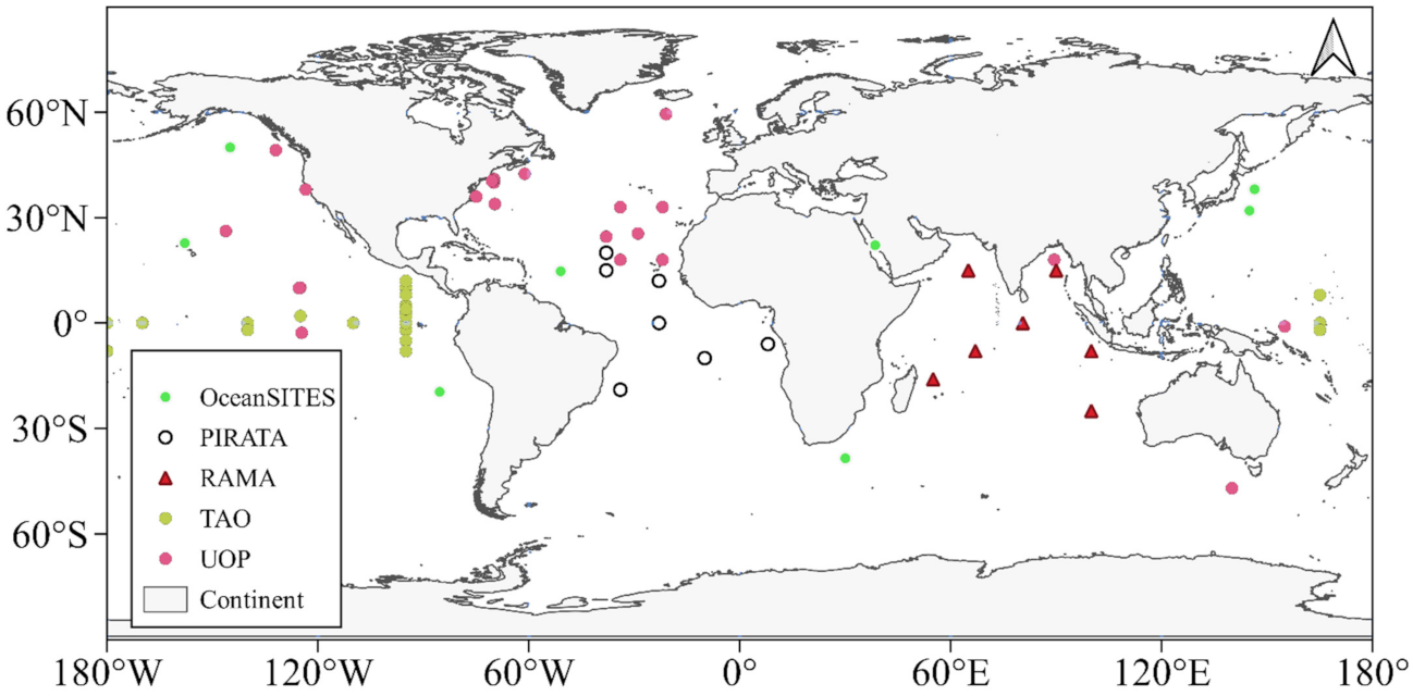
2.1. Measurements from Moored Buoy Sites

Radiative and meteorological observations from 66 moored buoy sites from 1988 to 2018 were collected and used in this study. Figure 1 shows the spatial distribution of the 66 moored buoy sites in five networks/projects, most of which were distributed in low- and mid-latitude oceans. However, only very few moored buoys were sparsely distributed in the mid–high latitude oceans in the Southern Hemisphere, which might be attributed to the presence of fewer “hot spots” for air–sea interactions in this region [31]. Fortunately, more buoys have been considered to be deployed at seas in the Southern Hemisphere, such as at the Brazil Current (55°–41°W, 48°–28°S) [32], the Eastern Australian Current (150°–165°E, 15°–45°S) [33], and so on. Hence, the performance of the new models developed in this study should be used for more investigations within this region in the future.

2.1.1. Introduction to the Moored Buoy Sites

Table 2 lists the detailed information about the five observation networks to which the moored buoy sites belong. The Upper Ocean Processes Group (UOP) launched by the Woods Hole Oceanographic Institution (WHOI) focuses on the study of physical processes in the upper ocean and at the air–sea interface using moored surface buoys equipped with meteorological and oceanographic sensors. These observations enable the first accurate quantification of the annual cycle of net air–sea heat exchange and wind stress from a Southern Ocean location [34]. Twenty-three sites for the UOP were collected. The Tropical Atmosphere Ocean/Triangle Trans-Ocean Buoy Network (TAO/TRITON) [24] in the tropical Pacific, The Pilot Research Moored Array in the Tropical Atlantic (PIRATA) [35] in the tropical Atlantic, and The Research Moored Array for African-Asian-Australian Monsoon (RAMA) [23] in the tropical Indian Ocean, were the components of the Global Tropical Moored Buoy Array (GTMBA) program deployed in the tropical oceans [36]. The data provided by the three networks have undergone extensive quality control examinations to ensure that they meet stringent accuracy standards [37,38], and they have been used in studies for understanding, monitoring and forecasting ENSO and ENSO-like events, meridional modes, and monsoon variability [23]. Thirty-five sites from the three networks were selected in this study (TAO: 21, PIRATA: 7, and RAMA: 7). The OceanSITES network consists of buoys funded by individual oceanographic investigators from many different nations. The aim of the OceanSITES network is to measure, deliver and promote the use of high-quality multidisciplinary data from long-term, high-frequency observations at fixed locations in the open ocean [12]. Eight sites from OceanSITES were used. Observations from 66 moored buoy sites have been widely applied in previous studies, such as air–sea interaction studies [13,39,40,41], ENSO prediction [42], and monsoon variability studies [23].
In general, the instruments for measuring the radiative components R g and R l were the Eppley Laboratory precision spectral pyranometer (PSP) and the precision infrared radiometer (PIR) with calibration accuracies of 2% and 1%, respectively [38]. According to previous study [12], the radiative flux measurements provided by the moored buoys are generally thought to be the highest-quality compared with those obtained from vessels; hence, the moored radiative measurements could be taken as the “ground truth” for tuning satellite measurements and assessing uncertainties in the surface flux estimates from satellites and models. For meteorological factors, RH and Ta were usually measured by the Rotronic Instrument corporation MP-101 temperature–humidity probe with accuracies of 2.7% and 0.2 K, respectively [38]. These radiative and meteorological sensors were deployed at a height of 3–5 m above the sea surface at the moored buoy site. To be different, the SST was measured under approximately 1 m of the ocean surface using Sea Bird Electronics (SBE37/39). As Table 2 shows, the observations from the different observation networks have different characteristics resulting from the different measurement instruments, data-processing procedures, quality-control policies, and so on; hence, all radiative and meteorological measurements were preprocessed first in the present study, and the details are given below.

2.1.2. Radiative Measurements

As mentioned above, only two downward radiations ( R g and R l ) were routinely measured at the ocean surface. Hence, the ocean surface Rn at moored buoys could be calculated by the following formulas [43,44]:
R ng = 1 α R g
R nl = R l ε ocean σ SST 4 + ( 1 ε ocean ) R l
where α is the daily ocean surface shortwave broadband albedo, ε ocean is the daily ocean surface broadband emissivity, and σ is the Stefan–Boltzmann’s constant ( 5 . 67   ×   10 8 W · m 2 · K 4 ).
From Equations (4) and (5), R g , R l , and SST can be measured directly, while the other two key parameters, α and εocean needed to be carefully defined for Rn calculation. In most previous studies, α and ε ocean were usually highly simplified in parameterizations using specific constants [28,45]. However, several recent studies have pointed out that the variations in α and εocean cannot be ignored, especially in the ocean surface energy balance calculation [12,46,47]. In this study, the α dataset from Feng et al. [48] during 2000–2018 and the ε ocean (8–13.5 μm) dataset from Cheng, Cheng, Liang, Niclòs, Nie and Liu [46] during 1981–2018, both with a 10 km spatial resolution at a daily scale, were used. The α dataset was generated using satellite reflectance data via MODIS and other ancillary information via MERRA reanalysis data based on a three-component reflectance model of ocean water, and its validation accuracy was generally consistent and satisfactory with the previous parameterization scheme [48]. The εocean dataset was generated based on its relationship with wind speed, and its validation accuracy was less than 0.003 under wind-free conditions at a daily scale, which was lower than the measurement uncertainty of 0.004 [46]. Hence, the employment of the two datasets was more reasonable. Note that the multiyear average daily α from 2000 to 2018 was used as the value for α before 2000 by considering the very small annual changes in α [49]. Furthermore, the buoy SST observations only represent the bulk SST because of the radiative cooling of the ocean surface skin; therefore, it is necessary to adjust the bulk SST measurements into ocean surface skin SST before Rn calculation. The bulk SST was closely related to the skin SST [50], the relationship was affected by wind speed, and a constant correction offset can be used as long as wind speed exceeds 6 m∙s−1 [51]. In fact, 83% of all samples were in a condition with wind speeds exceeding 4 m∙s−1, and the moored, measured bulk SST was directly adjusted to the skin SST by using a cooling bias of 0.17 K, as Vanhellemont [52] suggested. In this study, to obtain the daily ocean surface Rn at moored buoys, all measurements ( R g , R l , and adjusted SST) were aggregated into daily means from hourly values without any missing data and then fed into Equations (4) and (5). For those measurements at higher observation frequencies (i.e., 10 min), they were aggregated into hourly means first only when the available observations were more than five in one hour. Note that only the measurements flagged as high-quality were used in this study. Finally, the in situ ocean surface R g , R l , and Rn were obtained for modeling and validation afterwards. However, it is difficult to collect all inputs required in Equations (4) and (5), for instance, most moored buoys usually provide only one of the downward shortwave or longwave radiation measurements; therefore, an effective but more practical model for ocean surface Rn estimation is needed to meet the requirements of various studies and applications.

2.1.3. Meteorological and Other Ancillary Information

As Table 1 shows, three meteorological variables (Ta, RH, and ASTD) were also needed in this study. It is known that Ta is an essential parameter for radiation estimation. However, the difference between Ta and SST (ASTD) cannot be ignored for ocean surface net longwave radiation estimation. According to Fung et al. [53], the omission of ASTD could result in large net longwave radiation estimation errors in summer and winter for midlatitude and subarctic regions. Hence, the ASTD was taken into account for ocean surface Rn modeling in this study, as suggested by Clark, Eber, Laurs, Renner and Saur [45] and Bunker [54]. In addition, RH was also considered in this study because it is usually used as an indicator to capture the contribution of longwave radiation from moisture in the lower atmosphere [55,56,57,58]. The Ta and RH could be obtained directly from the moored buoy sites, and the ASTD was computed as the difference between the skin SST and Ta. As radiative measurements, the daily Ta, RH, and ASTD were also calculated from their hourly values.
In addition to the radiative and meteorological variables, the other two variables, Dd and CI (see Table 1), were needed for ocean surface Rn estimation model development. Dd is defined as the difference between sunrise and sunset, and the sunrise and sunset times were computed by using the National Oceanic and Atmospheric Administration’s (NOAA) Solar Calculation algorithm (NOAA Solar Calculator, www.esrl.noaa.gov/gmd/grad/solcalc/ (accessed on 15 October 2021)).
CI is the ratio of the surface downward solar radiation to the extraterrestrial solar radiation (DSRtoa), and it is usually used to represent sky conditions and atmospheric turbidity, which have significant influences on the surface radiative budget balance [20,41,59]. The CI value ranges from 0 to 1, and a larger CI indicates a clearer sky. CI has been successfully employed in previous studies [1,60,61,62] and is utilized in this study. CI can be calculated as following [1]:
CI = R g DSR toa
DSR toa = 1440 G sc d r π ω s sin φ sin δ + cos δ sin ω s
d r = 1 + 0 . 033 cos 2 π DOY 365
δ = 0 . 409 sin ( 2 π DOY 365 1 . 39 )
ω s   = cos 1 tan φ tan δ  
where G sc is the solar constant (1366.7 Wm−2), d r is the inverse relative distance from the Earth to the Sun, ω s is the sunset hour angle (rad), φ is the latitude (rad), δ is the sun declination (rad), and DOY is the day of the year. The CI calculated using the daily R g measurements at moored buoys was used for modeling.

2.1.4. Uncertainty Analysis

According to a previous study [63], the errors in the measurements at the ocean surface should be taken into account in modeling due to their relatively significant influences. Moreover, the in situ ocean surface Rn cannot be directly obtained at the moored buoy sites; therefore, its uncertainty should also be considered for better reference. According to the error propagation rules [64], the standard error of calculated Rn can be derived as:
S Y = j = 1 N Y X j S X j 2
where S is the standard error, Y is the dependent variable, X j is the independent variable in the formula, and N is the number of X. For example, if Y is the ocean surface Rn calculated by Equations (4) and (5), then N is equal to 5. This method is a general technique for estimating the moments of the variables under consideration. The first-order, second-moment, uncertainty analysis was used because Rn is a simple algebraic sum of radiative components. An implicit assumption of Equation (11) is that errors in different variables are independent. In this study, Equation (11) was applied to estimate the uncertainty of the in situ calculated ocean surface Rn, and it was extended and revised to estimate the uncertainty of the newly developed model by excluding the errors of all inputs.

2.2. CERES SYN1deg_Ed4A Product

For comparison, the daily R g and R l from the CERES SYN1deg_Ed4A product was utilized in the newly developed Rn estimation models. The CERES experiment provides Earth radiation budget data, including the top-of-atmosphere (TOA) radiation flux and surface radiation flux (https://ceres.larc.nasa.gov (accessed on 15 October 2021)). The CERES SYN1deg series product was calculated using the Langley Fu-Liou radiative transfer model from the input geostationary (GEO) radiance, MODIS and GEO cloud properties, Goddard Modeling and Assimilation Office (GMAO) atmospheric profiles, and MODIS aerosols [14]. Daily R g was computed by averaging the hourly R g and extracted according to the locations of the moored buoys.

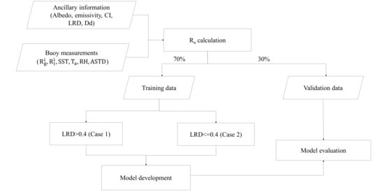
3. A New Ocean Surface Rn Empirical Estimation Scheme

As described above, the Rn at the land surface is closely related to the R g or R l determined by daytime duration [1,60,65], which has not been fully explored at the ocean surface. Hence, the relationships between the ocean surface Rn and its two components ( R g and R l ) were analyzed first before modeling. Based on the results, empirical models for Rn estimation were built and validated afterwards. In this study, the model accuracy is indicated by three statistical indices: root-mean-square-error (RMSE), mean bias error (bias) and R-squared (R2).

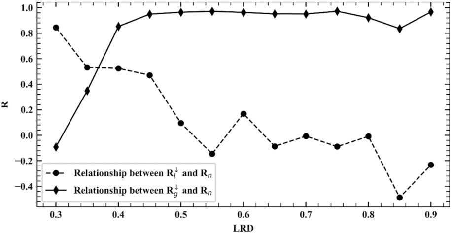
3.1. Relationships between the Ocean Surface Rn and R g / R l

Similar to the study by Chen, He, Jiang and Liang [65], the variations in the relationships between the ocean surface Rn and R g / R l with the length of daytime duration are explored. For convenience, a normalized index named the length ratio of daytime (LRD, 0 ~ 1), calculated using the ratio of the total daytime hours to the entire day (24 h), was used to represent daytime duration. The LRD was divided into 20 bins (by 0.05 increments), and then, the Pearson correlation (R) between the in situ daily ocean surface Rn and R g / R l was calculated for each LRD bin and is shown in Figure 2.
Figure 2 shows that the variations in the two relationships (Rn ~ R g and Rn ~ R l ) were opposite with increasing LRD. Specifically, the R values between the ocean surface Rn and R g (the solid dotted line) increased rapidly to approximately 0.84 when the LRD increased from 0.3 to 0.4, and the values remained very close to 1.0 afterwards, while the R values between the ocean surface Rn and R l (the dashed dotted line) decreased continuously from approximately 0.82 to 0 with LRD increasing from 0.3 to 0.55, and the values remained at approximately 0 or even lower afterwards. The two lines intersected when the LRD was approximately 0.4. The results indicate that the ocean surface Rn was highly correlated with the R g ( R l ) when the LRD was greater (less) than 0.4. Hence, it is more reasonable to estimate the ocean surface Rn under different conditions defined by the LRD.

3.2. Conditional Model Development

Many empirical models have been successfully developed for Rn estimation at the land surface directly from the R g   [1,60,66] when the two have a high correlation. Therefore, two conditional models were developed in this study in which the ocean surface Rn was estimated mainly from the ocean surface R g when the LRD was greater than 0.4 (hereinafter referred to as the Case 1 model), and mainly from the ocean surface R l when the LRD was equal to or less than 0.4 (hereinafter referred to as the Case 2 model). Table 3 shows the number of samples used for the two conditional model developments. Note that the samples for Case 2 modeling were much less than those for Case 1, because most moored buoys were located in low- and mid-latitude areas, where the LRD is usually larger than 0.4.

3.2.1. Case 1 Model

Figure 3 shows the scatter plot between the daily ocean surface Rn and R g when the LRD was greater than 0.4. The daily ocean surface Rn was highly linearly related to R g , with an R2 value of 0.925, RMSE of 15.501 Wm2, and bias of 0 Wm2 (Equation (12)). However, the linear relationship was not as good when the ocean surface Rn value was smaller than 100 Wm2.
R n = 0.846 R g 27.305
To improve the accuracy of the estimated Rn, other variables (see Table 1) were introduced into Equation (12). Therefore, the relationships between the model residuals R n 1   (the difference between the original and model estimates) from Equation (12) and these parameters were explored one by one. After multiple experiments, it was found that the RH, CI, and ASTD were related to the variations in R n 1 in different formats, as shown in Figure 4.
The scatter plots between the R n 1 and the CI, RH, and ASTD are shown in Figure 4a,c,e, respectively. To better display their relationships, the corresponding box plots are given in Figure 4b,d,f, respectively, in which the mean of the   R n 1 and its standard error of the mean (SEM) were calculated for each bin of the CI, RH, and ASTD (by 10% increments), respectively. Specifically, the R n 1   varied with the CI with a quadratic relationship (Figure 4b), and with the RH (Figure 4d) and ASTD (Figure 4f) in an approximate linear relationship. Hence, the CI, RH, and ASTD were introduced into Equation (12) in their proper formats as Equation (13):
R n = 1.05 R g + 0.83 RH 132.82 CI 2 + 17.15 CI + 3.58 ASTD 100.96
The training results of Equation (13) are shown in Figure 5. Compared with the fitting results from Equation (12) (Figure 3), the accuracy of the Rn estimations from the new model was significantly improved as the R2 value increased from 0.925 to 0.971 and the RMSE decreased from 15.501 Wm−2 to 9.650 Wm−2. Therefore, Equation (13) was determined as the Case 1 model.

3.2.2. Case 2 model

Figure 6 gives the scatter plot between the in situ daily ocean surface Rn and R l when the LRD ≤ 0.4. The daily ocean surface Rn is also linearly related to R l , although not as closely as the relationship between R g and Rn in Case 1. Similar to the Case 1 model development, a simple linear regression model (Equation (14)) taking R l as the only input, was built first. The fitting accuracy of Equation (14) was accepted with an R2 value of 0.558 and RMSE of 12.815 Wm−2.
R n = 0.568 R l 182.939
As in previous work, the relationships between the model residuals R n 2 from Equation (14) and the parameters in Table 1 were explored one by one, and two parameters (CI and Dd) were found to be linearly related to the variations in the R n 2 , as shown in Figure 7.
Therefore, the CI and Dd were directly introduced into Equation (14) as Equation (15):
R n = 0.839 R l + 7.125 Dd + 88.2 CI 354.93
Figure 8 shows that the fitting accuracy of Equation (15) was significantly improved compared with the results from Equation (14), by increasing the R2 value from 0.558 to 0.868 and decreasing the RMSE from 12.815 to 7.014 Wm−2, which indicated that the CI and Dd were very helpful in ocean surface Rn estimation when the LRD was small. It is known that the upward longwave radiation is mainly determined by SST; hence, SST should also be taken into account for estimating Rn under the Case 2 condition. Furthermore, a close linear relationship was found between the model residuals from Equation (15) ( R n 3 ) and the SST, as Figure 9 shows. Therefore, the final Case 2 model is given in Equation (16):
R n = 0.957 R l + 11.05 Dd + 102.323 CI 4.751 SST 393.461
The fitting results of Equation (16) are shown in Figure 10. Compared with Figure 6 and Figure 8, the results from Equation (16) were closer to the in situ ocean surface Rn, with an R2 value of 0.984 and an RMSE of 2.428 Wm−2. Therefore, Equation (16) was determined as the Case 2 model.
Overall, two conditional models (Case 1 and Case 2) for ocean surface Rn estimation were successfully built based on the measurements collected from more than 60 globally distributed moored buoys and in the formats of Equation (13) and Equation (16). Specifically, when the length of daytime duration is sufficiently large (LRD > 0.4), the daily ocean surface Rn is mainly determined by R g , and RH, CI and ASTD also make contributions. For other cases (LRD 0.4), the Case 2 model was formulated as a linear function of R l , Dd, CI and SST, and the fitting accuracies of both cases were satisfactory.

4. Results and Discussions

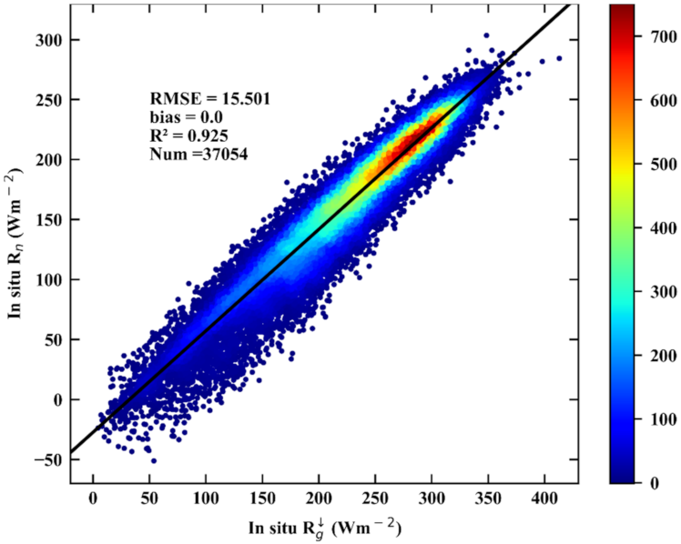
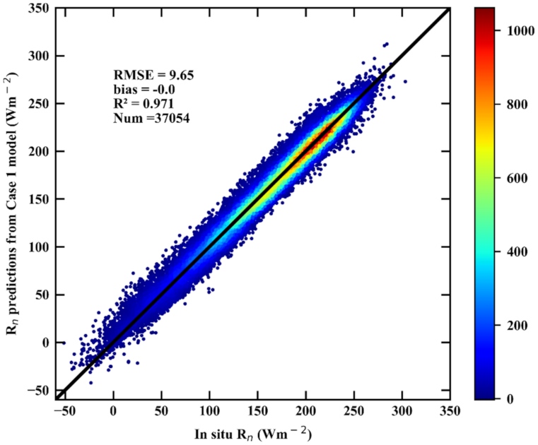
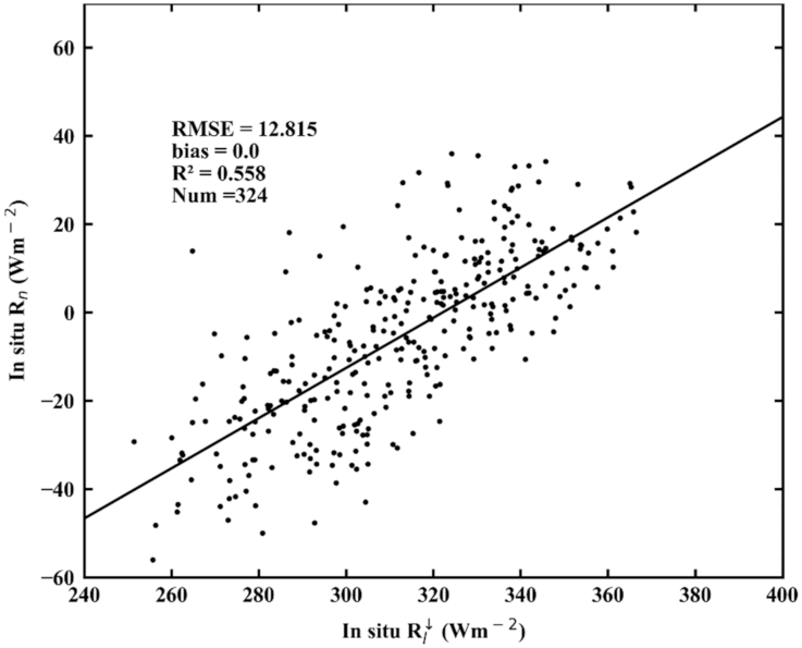
4.1. Validation Results

The overall accuracy of the ocean surface Rn estimations derived from the Case 1 and Case 2 models was validated against all independent validation samples (see Table 2), and the results are shown in Figure 11. Based on the results, the new ocean surface Rn empirical estimation scheme performed very well, with an R2 value of 0.972, an RMSE of 9.768 Wm−2, and a bias of −0.092 Wm−2. Moreover, the performances of the Case 1 and Case 2 models were also satisfactory, with R2 values of 0.972 and 0.979, RMSEs of 9.805 and 2.824 Wm−2, and biases of −0.095 and 0.346 Wm−2, respectively. For better illustration, validation was conducted at each moored buoy site. Figure 12 shows the spatial distribution of the validation accuracy for each moored buoy, represented by the RMSE value. Generally, the two models had better performances over the oceans in low-latitude areas than in mid- and high-latitude areas, especially over the open ocean. It was also found that the two conditional models performed more poorly over the ocean with high SSTs, where the variations in wind and atmospheric convection are more active because of intensive ocean–atmosphere interactions [67].
To further explore the influences of latitude and distance to the coastline on the performances of the newly developed models, the variations in the validation accuracy with the two factors were analyzed, and the results are presented in Figure 13 and Figure 14. By considering the different sizes of the samples, the relative RMSE (rRMSE) was used. In order to better illustrate the influence of the coastal seas on the model performance, the results in Figure 13 were calculated based on measurements only from the buoys over open seas, while the one in Figure 14 based on all available measurements. Figure 13 shows the performances of the new models in areas with different latitudes, which were classified into nine groups by latitude, in 10 degree intervals from 40°S to 50°N. The rRMSE and magnitude of the bias were both much lower over the oceans in low-latitude areas than in mid- and high-latitude areas. Similarly, the performances of the new models were examined by the distance to the coastline, from 0 to 300 km, as shown in Figure 14, and the closer to the coastline, the worse the validation accuracy of the new models. The results in Figure 13 and Figure 14 are consistent with the conclusions derived from Figure 12. On the one hand, this was possibly caused by the much higher number of samples available in low-latitude areas and open ocean for modeling, because the performance of the empirical model may tend to reflect highly sampled conditions. On the other hand, the atmospheric conditions, such as cloud characteristics, water vapor content, and aerosol types, are different for the areas near the coast and in low-latitude regions, which has not been thoroughly considered in the newly developed models. Specifically, the atmosphere over coastal ocean areas is usually affected by continental aerosols transported by favorable winds, which introduce more enhanced aerosol direct-radiative effects than over the open ocean [68,69].
Taking two moored buoy sites, TAO_03 (0°N, 140°W) and OS_PAPA (50°N, 145°W), as examples, TAO_03 is located in the tropical ocean, with all LRD values larger than 0.4, while OS_PAPA is located in the high-latitude ocean, with all LRD values smaller than 0.4 for some days in one year; thereby, only the Case 1 model was applied at TAO_03, but two conditional models were applied at OS_PAPA. The time series of the ocean surface Rn estimations and the moored Rn samples of the two sites, as well as their scatter plots, are shown in Figure 15. The ocean surface Rn estimations at the two sites captured the variations in the in situ Rn very well, and their validation results were very good, with R2 values of 0.927 and 0.984, RMSE values of 8.506 and 8.466 Wm−2, and bias values of 3.945 and −0.944 Wm−2, respectively.
Therefore, the direct validation results demonstrated the overall satisfactory performance of the newly developed models for ocean surface Rn estimation. However, the accuracy of the estimated ocean surface Rn obtained from the new models over the areas near the coast or at mid–high latitudes could be decreased because of the very limited number of samples available for modeling in these regions.

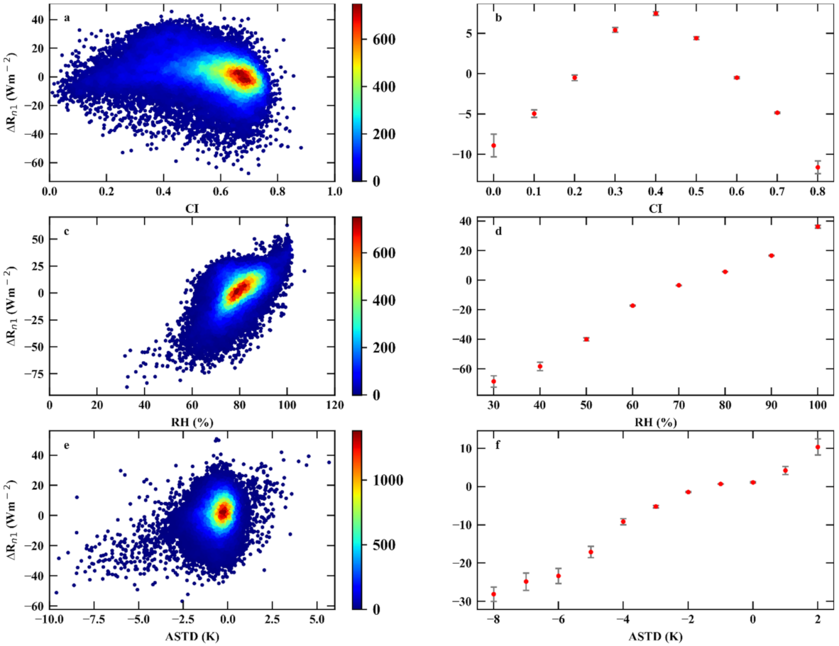
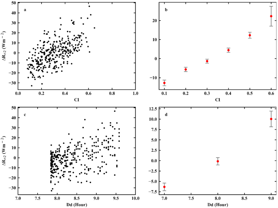
4.2. Model Sensitivity Analysis

To determine the effects of the input parameters on the estimated Rn from the Case 1 and Case 2 models, a global sensitivity analysis was conducted by utilizing SimLab software (http://simlab.jrc.ec.europa.eu (accessed on 15 October 2021)). All inputs into the Case 1 model ( R g , RH, CI and ASTD) and Case 2 model ( R l , CI, Dd and SST) were entered into SimLab separately, and then 4000 combinations of the inputs for the two models (2000 in Case 1 and 2000 in Case 2) were generated by assuming a normal distribution between the lower and upper bounds for each variable. Then, 4000 ocean surface Rn estimations were obtained from the Case 1 and Case 2 models with these generated combinations of inputs. Afterwards, all combinations of inputs and the corresponding ocean surface Rn estimations were used for sensitivity analysis using the Fourier amplitude sensitivity test (FAST) method [70] on the SimLab platform. The total sensitivity index (TSI), which indicated the total contribution of a factor to the output variance when the interactions of other factors were also computed, was employed to determine the sensitivity of each factor. Table 4 lists the TSI of each input in the Case 1 and Case 2 models. For the Case 1 model, R g played the most important role, with the largest TSI, 86.9%, and the second most sensitive variable was the CI with a TSI of 5.5%, while for the Case 2 model, R l was the most sensitive variable with a TSI of 64.3%, and the second most sensitive variable was also the CI with a contribution of 17.7% of the variance in the outputs. Therefore, the performances of the two newly developed models depended highly on the accuracies of the ocean surface R g and R l measurements, especially the R g , because of the importance of the CI in the two models.
To better understand the importance of the accuracy of R g and R l in the two conditional models, the validation accuracy of the estimated ocean surface Rn from the newly developed conditional models using the daily R g and R l from CERES SYN1deg_Ed4A (CERES R g and CERES R l ) were also examined. According to previous studies, the radiation product from CERES SYN1deg_Ed4A has been acknowledged to be one of the most reliable products for ocean surfaces [71]. In this study, the accuracy of CERES R g under the Case 1 condition was also validated against all independent validation samples with an R2 value of 0.818, an RMSE of 27.467 Wm2, and a bias of 0.971 Wm2. Additionally, the accuracy of CERES R l under the Case 2 condition was validated with an R2 value of 0.63, an RMSE of 15.672 Wm2, and a bias of 0.066 Wm2. Afterwards, the validation results of the estimated daily ocean surface Rn with the CERES R g and CERES R l (named CERES_based Rn for the Case 1 model and CERES_based Rn for the Case 2 model) are shown in Figure 16a,b, respectively. Note that the validation samples (14,185) for Case 1 were less than those in Figure 11 (15,952) because CERES_ R g has only been available since 2000. Hence, the validation accuracy of the Case 1 model with the in situ R g measurements since 2000 was calculated with an R2 value of 0.974, an RMSE of 9.035 Wm2, and a bias of −0.955 Wm2. Overall, the performances of the Case 1 and Case 2 models both worsened noticeably after replacing the in situ radiation measurements with those from CERES R g and CERES R l . Specifically, for the Case 1 model, the accuracy of the daily ocean surface Rn estimates worsened considerably using CERES R g , with an R2 value decreasing from 0.974 to 0.808 and RMSE increasing from 9.035 to 24.461 Wm2, respectively, while for the Case 2 model, the validated R2 value decreased from 0.979 to 0.453 and RMSE and bias increased from 2.824 to 14.825 and 0.346 to 1.113 Wm2, respectively. Therefore, reliable and accurate daily ocean surface R g and R l datasets are necessary for generating an accurate daily ocean surface Rn dataset.

4.3. Error Analysis

At the ocean surface, the errors in the moored buoy measurements mostly resulted from buoy rocking motions, sensor tilting due to wind and currents, solar contamination, thermal gradients in the dome and case temperatures, and dome contamination at sea (e.g., salt spray crystallization, bird guano, etc.) [37,72,73], and these errors in measurements have not been taken into account in the common validation (Section 4.1). Hence, the performance of the newly developed empirical models should be assessed by eliminating the influences of measurement errors in the inputs. A quantitative analysis of the error propagation of the new models was conducted in this section. In addition, the uncertainty in the in situ ocean surface Rn was estimated for comparison.
First, the variables related to error analysis are defined in Table 5.
P and O can be written as P = Ptr + Sp and O = Otr + So, and the uncertainty of the model is Sm = Ptr – Otr; hence, the residuals (∆P-O) between P and O are:
P-O = Sm + Sp − SO
By combining with the calculation of RMSE, we obtained ∆P-O ~ (0, 9.805) in the Case 1 model and ∆P-O ~ (0.346, 2.824) in the Case 2 model. Therefore, the Sm could be estimated if the uncertainty of Sp − SO ( S S P S O ) was known. According to the error propagation calculation (Equation (11) in Section 2.1.4) and the information provided in Table 6, S S P S O was 2.70 Wm−2 and 6.84 Wm−2 in the Case 1 and Case 2 models, respectively. Therefore, Smin the Case 1 or Case 2 model can be calculated as
S m = S P O 2 + S S P S O 2
Therefore, the “true” uncertainty of the Rn model was 10.17 Wm−2 and 6.84 Wm−2. For comparison, the uncertainty of the calculated in situ Rn using Equations (4) and (5) was estimated as 6.23 and 2.55 Wm−2 under the Case 1 and Case 2 conditions, respectively. Hence, the true uncertainty of the new model was comparable to the calculated in situ Rn, but takes more accessible buoy measurements as inputs, which demonstrated that the performance of the new model was satisfactory.

5. Conclusions

Ocean surface Rn is one of the most essential parameters in determining the ocean heat flux, which plays a vital role in controlling the stability of the Earth’s climate system. However, Rn, and four other radiative components are not routinely measured at the ocean surface; hence, a simple but effective ocean surface Rn estimation method is necessary for practical use. In this study, a new LRD-based empirical scheme for daily ocean surface Rn estimation was successfully developed based on downward shortwave or longwave radiation and meteorological measurements collected from more than 60 globally moored buoys.
The LRD-based empirical scheme includes two conditional models named Case 1 (Rn ~ f ( R g , CI, RH, ASTD)) and Case 2 (Rn ~f ( R l , CI, Dd, SST)). Specifically, when the length of daytime duration was longer than 9.6 hours (LRD > 0.4), the ocean surface Rn was primarily determined by R g , while the ocean surface Rn was primarily determined by R l for the other cases. After validation against the in situ ocean surface Rn calculations, the overall accuracy of the new scheme was very good with an R2 value of 0.972, an RMSE of 9.768 Wm−2, and a bias of −0.092 Wm−2, and the performance of the two conditional models was also satisfactory, with R2 values of 0.972 and 0.979, RMSE values of 9.805 and 2.824 Wm−2, and bias values of −0.095 and 0.346 Wm−2, respectively. Afterwards, the “true” performance of the Case 1 and Case 2 models was estimated by eliminating the measurement errors in the inputs, which were also very good, with uncertainties of 10.17 and 6.84 Wm−2, respectively. These were comparable to the uncertainties of the calculated in situ ocean surface Rn of 6.23 and 2.55 Wm−2 under Case 1 and Case 2 conditions, respectively, but with a simpler format and more easily accessible inputs. Therefore, the new empirical LRD-based scheme for ocean surface Rn has strong potential to be widely used in the near future.
However, some drawbacks in the newly developed models should be noted. For example, the two models performed worse in areas near the coastline and at high latitudes because of the limited number of samples collected within these regions, and the accuracy in the Rn estimates strongly depends on the accuracies of R g and R l . Furthermore, the models only work as long as the CI is available, which indicates that the new models cannot work when the daytime length is short (LRD = 0.3 in this study). More efforts should be made to improve the performance and robustness of the newly developed models in future research.

Author Contributions

Conceptualization, J.P. and B.J.; methodology, J.P.; software, J.P.; validation, J.P., B.J. and H.C.; formal analysis, H.L.; investigation, S.L. (Shaopeng Li); resources, J.H.; data curation, Q.L.; writing—original draft preparation, J.P.; writing—review and editing, B.J.; visualization, J.C.; supervision, K.J., Y.Y. and X.Z.; project administration, S.L. (Shunlin Liang); funding acquisition, S.L. (Shunlin Liang) and B.J. All authors have read and agreed to the published version of the manuscript.

Funding

This research was funded by the Chinese Grand Research Program on Climate Change and Responses (Grant No. 2016YFA0600101) and Natural Science Foundation of China (Grant No. 41971291).

Data Availability Statement

Data available on request.

Acknowledgments

We acknowledge the moored buoy data provided by the Upper Ocean Process Group of the Woods Hole Oceanographic Institution (UOP); the GTMBA Project Office of NOAA/PMEL; and the international OceanSITES project and the national programs that contributed to these data sets. We are also grateful to NASA and NOAA for providing the satellite products. Acknowledgement for the data support from “National Earth System Science Data Center, National Science & Technology Infrastructure of China. (http://www.geodata.cn (accessed on 15 October 2021)).

Conflicts of Interest

The authors declare no conflict of interest.

References

  1. Jiang, B.; Zhang, Y.; Liang, S.; Wohlfahrt, G.; Arain, A.; Cescatti, A.; Georgiadis, T.; Jia, K.; Kiely, G.; Lund, M.; et al. Empirical estimation of daytime net radiation from shortwave radiation and ancillary information. Agric. For. Meteorol. 2015, 211–212, 23–36. [Google Scholar] [CrossRef] [Green Version]
  2. Tomita, H.; Hihara, T.; Kako, S.I.; Kubota, M.; Kutsuwada, K. An introduction to J-OFURO3, a third-generation Japanese ocean flux data set using remote-sensing observations. J. Oceanogr. 2019, 75, 171–194. [Google Scholar] [CrossRef] [Green Version]
  3. Trenberth, K.E.; Fasullo, J.T.; Balmaseda, M.A. Earth’s energy imbalance. J. Clim. 2014, 27, 3129–3144. [Google Scholar] [CrossRef] [Green Version]
  4. Fujii, Y.; Tsujino, H.; Toyoda, T.; Nakano, H. Enhancement of the southward return flow of the Atlantic Meridional Overturning Circulation by data assimilation and its influence in an assimilative ocean simulation forced by CORE-II atmospheric forcing. Clim. Dyn. 2015, 49, 869–889. [Google Scholar] [CrossRef]
  5. Wunsch, C. The total meridional heat flux and its oceanic and atmospheric partition. J. Clim. 2005, 18, 4374–4380. [Google Scholar] [CrossRef] [Green Version]
  6. Stephens, G.L.; Li, J.; Wild, M.; Clayson, C.A.; Loeb, N.; Kato, S.; L’Ecuyer, T.; Stackhouse, P.W., Jr.; Lebsock, M.; Andrews, T. An update on Earth’s energy balance in light of the latest global observations. Nat. Geosci. 2012, 5, 691–696. [Google Scholar] [CrossRef]
  7. Wild, M.; Folini, D.; Schar, C.; Loeb, N.; Dutton, E.G.; Konig-Langlo, G. The global energy balance from a surface perspective. Clim. Dyn. 2013, 40, 3107–3134. [Google Scholar] [CrossRef] [Green Version]
  8. Trenberth, K.E.; Caron, J.M. Estimates of meridional atmosphere and ocean heat transports. J. Clim. 2001, 14, 3433–3443. [Google Scholar] [CrossRef]
  9. Baggenstos, D.; Haberli, M.; Schmitt, J.; Shackleton, S.A.; Birner, B.; Severinghaus, J.P.; Kellerhals, T.; Fischer, H. Earth’s radiative imbalance from the Last Glacial Maximum to the present. Proc. Natl. Acad. Sci. USA 2019, 116, 14881–14886. [Google Scholar] [CrossRef] [Green Version]
  10. Hansen, J.; Sato, M.; Kharecha, P.; Schuckmann, K.V. Earth’s energy imbalance and implications. Atmos. Chem. Phys. 2011, 11, 13421–13449. [Google Scholar] [CrossRef] [Green Version]
  11. von Schuckmann, K.; Palmer, M.D.; Trenberth, K.E.; Cazenave, A.; Chambers, D.; Champollion, N.; Hansen, J.; Josey, S.A.; Loeb, N.; Mathieu, P.P.; et al. An imperative to monitor Earth’s energy imbalance. Nat. Clim. Chang. 2016, 6, 138–144. [Google Scholar] [CrossRef] [Green Version]
  12. Cronin, M.F.; Gentemann, C.L.; Edson, J.; Ueki, I.; Bourassa, M.; Brown, S.; Clayson, C.A.; Fairall, C.W.; Farrar, J.T.; Gille, S.T.; et al. Air-sea fluxes with a focus on heat and momentum. Front. Mar. Sci. 2019, 6, 430. [Google Scholar] [CrossRef] [Green Version]
  13. Pinker, R.T.; Bentamy, A.; Katsaros, K.B.; Ma, Y.; Li, C. Estimates of net heat fluxes over the Atlantic Ocean. J. Geophys. Res.-Oceans 2014, 119, 410–427. [Google Scholar] [CrossRef] [Green Version]
  14. Wielicki, B.A.; Barkstrom, B.R.; Baum, B.A.; Charlock, T.P.; Green, R.N.; Kratz, D.P.; Lee, R.B.; Minnis, P.; Smith, G.L.; Takmeng, W.; et al. Clouds and the Earth’s radiant energy system (CERES): Algorithm overview. IEEE Trans. Geosci. Remote Sens. 1998, 36, 1127–1141. [Google Scholar] [CrossRef] [Green Version]
  15. Rossow, W.B.; Zhang, Y.C. Calculation of surface and top of atmosphere radiative fluxes from physical quantities based on ISCCP data sets: 2. Validation and first results. J. Geophys. Res.-Atmos. 1995, 100, 1167–1197. [Google Scholar] [CrossRef]
  16. Dee, D.P.; Uppala, S.M.; Simmons, A.J.; Berrisford, P.; Poli, P.; Kobayashi, S.; Andrae, U.; Balmaseda, M.A.; Balsamo, G.; Bauer, P.; et al. The ERA-Interim reanalysis: Configuration and performance of the data assimilation system. Q. J. R. Meteorol. Soc. 2011, 137, 553–597. [Google Scholar] [CrossRef]
  17. Berry, D.I.; Kent, E.C. Air-sea fluxes from ICOADS: The construction of a new gridded dataset with uncertainty estimates. Int. J. Climatol. 2011, 31, 987–1001. [Google Scholar] [CrossRef]
  18. Jin, X.; Weller, R.A. Multidecade Global Flux Datasets from the Objectively Analyzed Air-Sea Fluxes (Oaflux) Project: Latent and Sensible Heat Fluxes, Ocean Evaporation, and Related Surface Meteorological Variables Lisan Yu; OAFlux Project Technical Report (OA-2008-01); NOAA: Washington, DC, USA, 2008; Volume 74, pp. 1–64. [Google Scholar]
  19. Kaminsky, K.Z.; Dubayah, R. Estimation of surface net radiation in the boreal forest and northern prairie from shortwave flux measurements. J. Geophys. Res.-Atmos 1997, 102, 29707–29716. [Google Scholar] [CrossRef]
  20. Iziomon, M.G.; Mayer, H.; Matzarakis, A. Empirical models for estimating net radiative flux: A case study for three mid-latitude sites with orographic variability. Astrophys. Space Sci. 2000, 273, 313–330. [Google Scholar] [CrossRef]
  21. Jiang, B.; Liang, S.; Jia, A.; Xu, J.; Zhang, X.; Xiao, Z.; Zhao, X.; Jia, K.; Yao, Y. Validation of the surface daytime net radiation product from version 4.0 GLASS product suite. IEEE Geosci. Remote Sens. Lett. 2019, 16, 509–513. [Google Scholar] [CrossRef]
  22. Polavarapu, R.J. Estimation of net radiation at sea. Atmos.-Ocean 1979, 17, 24–35. [Google Scholar] [CrossRef] [Green Version]
  23. McPhaden, M.J.; Meyers, G.; Ando, K.; Masumoto, Y.; Murty, V.S.N.; Ravichandran, M.; Syamsudin, F.; Vialard, J.; Yu, L.; Yu, W. RAMA: The research moored array for African–Asian–Australian monsoon analysis and prediction. Bull. Am. Meteorol. Soc. 2009, 90, 459–480. [Google Scholar] [CrossRef] [Green Version]
  24. McPhaden, M.J.; Busalacchi, A.J.; Cheney, R.; Donguy, J.R.; Gage, K.S.; Halpern, D.; Ji, M.; Julian, P.; Meyers, G.; Mitchum, G.T.; et al. The Tropical Ocean-Global Atmosphere observing system: A decade of progress. J. Geophys. Res.-Oceans 1998, 103, 14169–14240. [Google Scholar] [CrossRef]
  25. Lumb, F.E. The influence of cloud on hourly amounts of total solar radiation at the sea surface. Q. J. R. Meteorol. Soc. 1964, 90, 43–56. [Google Scholar] [CrossRef]
  26. Dobson, F.W.; Smith, S.D. A comparison of incoming solar radiation at marine and continental stations. Q. J. R. Meteorol. Soc. 1989, 115, 353–364. [Google Scholar] [CrossRef]
  27. Kalisch, J.; Macke, A. Estimation of the total cloud cover with high temporal resolution and parametrization of short-term fluctuations of sea surface insolation. Meteorol. Z. 2008, 17, 603–611. [Google Scholar] [CrossRef] [Green Version]
  28. Bignami, F.; Marullo, S.; Santoleri, R.; Schiano, M.E. Longwave radiation budget in the Mediterranean Sea. J. Geophys. Res.-Oceans 1995, 100, 2501–2514. [Google Scholar] [CrossRef]
  29. Josey, S.A.; Oakley, D.; Pascal, R.W. On estimating the atmospheric longwave flux at the ocean surface from ship meteorological reports. J. Geophys. Res.-Oceans 1997, 102, 27961–27972. [Google Scholar] [CrossRef]
  30. Josey, S.A.; Gulev, S.; Yu, L. Exchanges through the ocean surface. Int. Geophys. 2013, 103, 115–140. [Google Scholar] [CrossRef]
  31. Yang, H.; Lohmann, G.; Wei, W.; Dima, M.; Ionita, M.; Liu, J. Intensification and poleward shift of subtropical western boundary currents in a warming climate. J. Geophys. Res.-Oceans 2016, 121, 4928–4945. [Google Scholar] [CrossRef] [Green Version]
  32. Franz, G.; Garcia, C.A.E.; Pereira, J.; de Freitas Assad, L.P.; Rollnic, M.; Garbossa, L.H.P.; da Cunha, L.C.; Lentini, C.A.D.; Nobre, P.; Turra, A.; et al. Coastal Ocean Observing and Modeling Systems in Brazil: Initiatives and Future Perspectives. Front. Mar. Sci. 2021, 8, 1038. [Google Scholar] [CrossRef]
  33. Roughan, M.; Morris, B.D.; Suthers, I.M. NSW-IMOS: An integrated marine observing system for southeastern Australia. In IOP Conference Series: Earth and Environmental Science; IOP Publishing: Bristol, UK, 2010; p. 012030. [Google Scholar]
  34. Schulz, E.W.; Josey, S.A.; Verein, R. First air-sea flux mooring measurements in the Southern Ocean. Geophys. Res. Lett. 2012, 39. [Google Scholar] [CrossRef]
  35. Bourlès, B.; Lumpkin, R.; McPhaden, M.J.; Hernandez, F.; Nobre, P.; Campos, E.; Yu, L.; Planton, S.; Busalacchi, A.; Moura, A.D. The PIRATA program: History, accomplishments, and future directions. Bull. Am. Meteorol. Soc. 2008, 89, 1111–1126. [Google Scholar] [CrossRef]
  36. McPhaden, M.J.; Ando, K.; Bourlès, B.; Freitag, H.P.; Lumpkin, R.; Masumoto, Y.; Murty, V.S.N.; Nobre, P.; Ravichandran, M.; Vialard, J.; et al. The global tropical moored buoy array. Proc. OceanObs 2010, 9, 668–682. [Google Scholar] [CrossRef] [Green Version]
  37. Medovaya, M.; Waliser, D.E.; Weller, R.A.; McPhaden, M.J. Assessing ocean buoy shortwave observations using clear-sky model calculations. J. Geophys. Res. 2002, 107. [Google Scholar] [CrossRef] [Green Version]
  38. Lake, B.J. Calibration Procedures and Instrumental Accuracy Estimates of ATLAS Air Temperature and Relative Humidity Measurements; NOAA Tech Memo. OAR PMEL-123; NOAA/Pacific Marine Environmental Laboratory: Seattle, WA, USA, 2003; p. 23. [Google Scholar]
  39. May, J.C.; Rowley, C.; Barron, C.N. NFLUX satellite-based surface radiative heat fluxes. part II: Gridded products. J. Appl. Meteorol. Climatol. 2017, 56, 1043–1057. [Google Scholar] [CrossRef] [Green Version]
  40. Cronin, M.F.; Fairall, C.W.; McPhaden, M.J. An assessment of buoy-derived and numerical weather prediction surface heat fluxes in the tropical Pacific. J. Geophys. Res.-Oceans 2006, 111, 6. [Google Scholar] [CrossRef]
  41. Cronin, M.F.; McPhaden, M.J. The upper ocean heat balance in the western equatorial Pacific warm pool during September–December 1992. J. Geophys. Res.-Oceans 1997, 102, 8533–8553. [Google Scholar] [CrossRef]
  42. Petrova, D.; Ballester, J.; Koopman, S.J.; Rodó, X. Multiyear statistical prediction of ENSO enhanced by the tropical Pacific observing system. J. Clim. 2020, 33, 163–174. [Google Scholar] [CrossRef] [Green Version]
  43. Praveen Kumar, B.; Vialard, J.; Lengaigne, M.; Murty, V.S.N.; McPhaden, M.J. TropFlux: Air-sea fluxes for the global tropical oceans—description and evaluation. Clim. Dyn. 2011, 38, 1521–1543. [Google Scholar] [CrossRef]
  44. Xu, J.; Jiang, B.; Liang, S.; Li, X.; Wang, Y.; Peng, J.; Chen, H.; Liang, H.; Li, S. Generating a High-Resolution Time-Series Ocean Surface Net Radiation Product by Downscaling J-OFURO3. IEEE Trans. Geosci. Remote Sens. 2020, 59, 2794–2809. [Google Scholar] [CrossRef]
  45. Clark, N.E.; Eber, L.; Laurs, R.M.; Renner, J.A.; Saur, J.F.T. Heat Exchange between Ocean and Atmosphere in the Eastern North Pacific for 1961–1971; Technical Report NMFS SSRF-682; NOAA, U.S. Department of Commerce: Washington, DC, USA, 1974. [Google Scholar]
  46. Cheng, J.; Cheng, X.; Liang, S.; Niclòs, R.; Nie, A.; Liu, Q. A lookup table-based method for estimating sea surface hemispherical broadband emissivity values (8–13.5 μm). Remote Sens. 2017, 9, 245. [Google Scholar] [CrossRef] [Green Version]
  47. Hogikyan, A.; Cronin, M.F.; Zhang, D.; Kato, S. Uncertainty in net surface heat flux due to differences in commonly used albedo products. J. Clim. 2020, 33, 303–315. [Google Scholar] [CrossRef]
  48. Feng, Y.; Liu, Q.; Qu, Y.; Liang, S. Estimation of the ocean water albedo from remote sensing and meteorological reanalysis data. IEEE Trans. Geosci. Remote Sens. 2015, 54, 850–868. [Google Scholar] [CrossRef]
  49. Jin, Z.; Charlock, T.P.; Smith, W.L.; Rutledge, K. A parameterization of ocean surface albedo. Geophys. Res. Lett 2004, 31. [Google Scholar] [CrossRef]
  50. Donlon, C.J.; Minnett, P.J.; Gentemann, C.; Nightingale, T.J.; Barton, I.J.; Ward, B.; Murray, M.J. Toward improved validation of satellite sea surface skin temperature measurements for climate research. J. Clim. 2002, 15, 353–369. [Google Scholar] [CrossRef] [Green Version]
  51. Alappattu, D.P.; Wang, Q.; Yamaguchi, R.; Lind, R.J.; Reynolds, M.; Christman, A.J. Warm layer and cool skin corrections for bulk water temperature measurements for air-sea interaction studies. J. Geophys. Res.-Oceans 2017, 122, 6470–6481. [Google Scholar] [CrossRef]
  52. Vanhellemont, Q. Automated water surface temperature retrieval from Landsat 8/TIRS. Remote Sens. Environ. 2020, 237, 111518. [Google Scholar] [CrossRef]
  53. Fung, I.Y.; Harrison, D.; Lacis, A.A. On the variability of the net longwave radiation at the ocean surface. Rev. Geophys. 1984, 22, 177–193. [Google Scholar] [CrossRef]
  54. Bunker, A.F. Computations of surface energy flux and annual air–sea interaction cycles of the North Atlantic Ocean. Mon. Weather Rev. 1976, 104, 1122–1140. [Google Scholar] [CrossRef] [Green Version]
  55. Gupta, S.K.; Kratz, D.P.; Stackhouse, P.W.; Wilber, A.C.; Zhang, T.; Sothcott, V.E. Improvement of surface longwave flux algorithms used in CERES processing. J. Appl. Meteorol. Climatol. 2010, 49, 1579–1589. [Google Scholar] [CrossRef]
  56. Swinbank, W.C. Longwave radiation from clear skies. Q. J. R. Meteorol. Soc. 1963, 89, 339–348. [Google Scholar] [CrossRef]
  57. Idso, S.B.; Jackson, R.D. Thermal radiation from the atmosphere. J. Geophys. Res. 1969, 74, 5397–5403. [Google Scholar] [CrossRef]
  58. Cheng, J.; Liang, S.; Wang, W.; Guo, Y. An efficient hybrid method for estimating clear-sky surface downward longwave radiation from MODIS data. J. Geophys. Res.-Atmos. 2017, 122, 2616–2630. [Google Scholar] [CrossRef]
  59. Boilley, A.; Wald, L. Comparison between meteorological re-analyses from ERA-Interim and MERRA and measurements of daily solar irradiation at surface. Renew. Energy 2015, 75, 135–143. [Google Scholar] [CrossRef]
  60. Jiang, B.; Liang, S.; Ma, H.; Zhang, X.; Xiao, Z.; Zhao, X.; Jia, K.; Yao, Y.; Jia, A. GLASS daytime all-wave net radiation product: Algorithm development and preliminary validation. Remote Sens. 2016, 8, 222. [Google Scholar] [CrossRef] [Green Version]
  61. Payne, R.E. Albedo of the sea surface. J. Atmos. Sci. 1972, 29, 959–970. [Google Scholar] [CrossRef]
  62. Iziomon, M.G.; Mayer, H.; Matzarakis, A. Downward atmospheric longwave irradiance under clear and cloudy skies: Measurement and parameterization. J. Atmos. Sol.-Terr. Phys. 2003, 65, 1107–1116. [Google Scholar] [CrossRef]
  63. Foltz, G.R.; Evan, A.T.; Freitag, H.P.; Brown, S.; McPhaden, M.J. Dust accumulation biases in PIRATA shortwave radiation records. J. Atmos. Ocean. Technol. 2013, 30, 1414–1432. [Google Scholar] [CrossRef] [Green Version]
  64. Taylor, J.R. Error Analysis; Univ. Science Books: Sausalito, CA, USA, 1997. [Google Scholar]
  65. Chen, J.; He, T.; Jiang, B.; Liang, S. Estimation of all-sky all-wave daily net radiation at high latitudes from MODIS data. Remote Sens. Environ. 2020, 245, 111842. [Google Scholar] [CrossRef]
  66. Wang, K.C.; Liang, S.L. Estimation of daytime net radiation from shortwave radiation measurements and meteorological observations. J. Appl. Meteorol. Climatol. 2009, 48, 634–643. [Google Scholar] [CrossRef]
  67. Wang, C.; Enfield, D.B. The tropical Western Hemisphere warm pool. Geophys. Res. Lett. 2001, 28, 1635–1638. [Google Scholar] [CrossRef]
  68. Meloni, D. Tropospheric aerosols in the Mediterranean: 2. Radiative effects through model simulations and measurements. J. Geophys. Res. 2003, 108. [Google Scholar] [CrossRef]
  69. Nair, V.S.; Babu, S.S.; Satheesh, S.K.; Moorthy, K.K. Effects of sea surface winds on marine aerosols characteristics and impacts on longwave radiative forcing over the Arabian Sea. Atmos. Chem. Phys. 2008, 8, 15855–15899. [Google Scholar] [CrossRef]
  70. Tarantola, S.; Chan, K.P.S.; Saltelli, A.; Chan, K.P.S. A Quantitative Model-Independent Method for Global Sensitivity Analysis of Model Output. Technometrics 1999, 41, 39–56. [Google Scholar] [CrossRef]
  71. Thandlam, V.; Rahaman, H. Evaluation of surface shortwave and longwave downwelling radiations over the global tropical oceans. SN Appl. Sci. 2019, 1, 1171. [Google Scholar] [CrossRef] [Green Version]
  72. Colbo, K.; Weller, R.A. Accuracy of the IMET sensor package in the subtropics. J. Atmos. Ocean. Technol. 2009, 26, 1867–1890. [Google Scholar] [CrossRef] [Green Version]
  73. Macwhorter, M.A.; Weller, R.A. Error in measurements of incoming shortwave radiation made from ships and buoys. J. Atmos. Ocean. Technol. 1991, 8, 108–117. [Google Scholar] [CrossRef]
Figure 1. Spatial distribution of the 66 moored buoy sites from five observation networks.
Remotesensing 13 04170 g001
Figure 2. The correlation between Rn and R g and R l with LRD.
Remotesensing 13 04170 g002
Figure 3. Scatter plot showing relationship between the in situ daily ocean surface Rn and R g .
Remotesensing 13 04170 g003
Figure 4. The scatter plots showing relationships between the model residuals R n 1 from Equation (12) and (a) CI, (c) RH and (e) ASTD, and (b), (d) and (f) are their corresponding box plots.
Remotesensing 13 04170 g004
Figure 5. Fitting results of the Case 1 model.
Remotesensing 13 04170 g005
Figure 6. Scatter plot showing relationship between the in situ daily ocean surface Rn and R l .
Remotesensing 13 04170 g006
Figure 7. The same as Figure 4 but for the model residuals R n 2 and CI and Dd.
Remotesensing 13 04170 g007
Figure 8. Fitting accuracy of Equation (15).
Remotesensing 13 04170 g008
Figure 9. The same as Figure 4 but for the model residuals R n 3 and SST.
Remotesensing 13 04170 g009
Figure 10. Fitting accuracy of the Case 2 model (Equation (16)).
Remotesensing 13 04170 g010
Figure 11. Overall validation results of the newly developed models.
Remotesensing 13 04170 g011
Figure 12. Validation accuracy of the newly developed models at each moored buoy site, represented by the RMSE value.
Remotesensing 13 04170 g012
Figure 13. The performances of the new models in oceans within different latitudinal zones.
Remotesensing 13 04170 g013
Figure 14. The same as Figure 13 but for different distances to the coastline.
Remotesensing 13 04170 g014
Figure 15. Time series and scatter plots of the ocean surface Rn estimations and the in situ Rn at the (a,b) TAO_03 (0°N, 140°W) and (c,d) OS_PAPA (50°N, 145°W) sites.
Remotesensing 13 04170 g015
Figure 16. Validation results of CERES-based Rn estimates.
Remotesensing 13 04170 g016
Table 1. Variables used for modeling in this study.
AbbreviationVariableUnitSource
Independent variables R l Daily downward longwave radiationWm2In situ
R g Daily surface incoming solar radiationWm2In situ/CERES
RHDaily mean relative humidity%In situ
SST 1Daily mean sea surface temperatureKIn situ
TaDaily air temperatureKIn situ
ASTDAir–sea temperature differenceKCalculated
CIClearness index Calculated
DdDaytime durationHourCalculated
Dependent variable RnDaily ocean-surface net radiationWm2Calculated
1 SST was corrected from the measured bulk sea surface temperature.
Table 2. Descriptions of each network.
Network/ProgramNumber of SitesPeriodObservation FrequencyURL
UOP231988–20171 hhttp://uop.whoi.edu/index.html (accessed on 15 October 2021)
TAO/TRITON212000–201910 minhttps://www.pmel.noaa.gov/tao/drupal/disdel/ (accessed on 15 October 2021)
RAMA72004–201810 minhttps://www.pmel.noaa.gov/tao/drupal/disdel/ (accessed on 15 October 2021)
PIRATA72006–201710 minhttps://www.pmel.noaa.gov/tao/drupal/disdel/ (accessed on 15 October 2021)
OceanSITES82000–20191 hhttp://www.oceansites.org/ (accessed on 15 October 2021)
Table 3. Details of the two conditional models for Rn estimation.
Conditional ModelClassification CriteriaTraining SamplesValidation Samples
Case 1LRD > 0.437,05415,952
Case 2LRD <= 0.4 324130
Table 4. The total sensitivity index of each input in Case 1 and Case 2.
Model R g R l RHCIASTDDdSST
Case 10.869\0.0310.0550.003\\
Case 2\0.643\0.177\0.0530.052
Table 5. Variable definitions.
AbbreviationStands for
POcean surface Rn estimations
OIn situ ocean surface Rn calculations
P tr Ocean surface Rn estimations with “true” inputs
O tr In situ ocean surface Rn without measurement errors (true values)
S p Uncertainty of the ocean surface Rn estimations
S o Uncertainty of the in situ ocean surface Rn calculations
S m Uncertainty of the model
Table 6. The standard error of each parameter.
ParametersCase 1 Standard Error\AverageCase 2 Standard Error\AverageSource
R g (Wm2)6\225.40 0.90\33.90[72]
R l (Wm2)2.5\397.02.5\310.99 [72]
RH (%)0.027\--\-[38]
CI0.015\0.570.06\0.31Calculated
ASTD (K)0.20\--\-[72]
Dd (Hour)-\-0\-Calculated
SST (K)0.07\298.200.07\280.63[50]
α 0.0049\0.060.0049\0.06[48]
ε ocean 0.002\0.950.002\0.95[46]
Publisher’s Note: MDPI stays neutral with regard to jurisdictional claims in published maps and institutional affiliations.

