A Training Sample Migration Method for Wetland Mapping and Monitoring Using Sentinel Data in Google Earth Engine

Abstract

Wetlands are one of the most important ecosystems due to their critical services to both humans and the environment. Therefore, wetland mapping and monitoring are essential for their conservation. In this regard, remote sensing offers efficient solutions due to the availability of cost-efficient archived images over different spatial scales. However, a lack of sufficient consistent training samples at different times is a significant limitation of multi-temporal wetland monitoring. In this study, a new training sample migration method was developed to identify unchanged training samples to be used in wetland classification and change analyses over the International Shadegan Wetland (ISW) areas of southwestern Iran. To this end, we first produced the wetland map of a reference year (2020), for which we had training samples, by combining Sentinel-1 and Sentinel-2 images and the Random Forest (RF) classifier in Google Earth Engine (GEE). The Overall Accuracy (OA) and Kappa coefficient (KC) of this reference map were 97.93% and 0.97, respectively. Then, an automatic change detection method was developed to migrate unchanged training samples from the reference year to the target years of 2018, 2019, and 2021. Within the proposed method, three indices of the Normalized Difference Vegetation Index (NDVI), Normalized Difference Water Index (NDWI), and the mean Standard Deviation (SD) of the spectral bands, along with two similarity measures of the Euclidean Distance (ED) and Spectral Angle Distance (SAD), were computed for each pair of reference–target years. The optimum threshold for unchanged samples was also derived using a histogram thresholding approach, which led to selecting the samples that were most likely unchanged based on the highest OA and KC for classifying the test dataset. The proposed migration sample method resulted in high OAs of 95.89%, 96.83%, and 97.06% and KCs of 0.95, 0.96, and 0.96 for the target years of 2018, 2019, and 2021, respectively. Finally, the migrated samples were used to generate the wetland map for the target years. Overall, our proposed method showed high potential for wetland mapping and monitoring when no training samples existed for a target year.

1. Introduction

Wetlands are valuable ecosystems and offer important services to both nature and human beings. For example, they play a key role in water purification, carbon cycles, flood and storm control, soil erosion control, and providing wildlife habitats [1,2,3,4,5]. Despite these benefits, a significant portion of wetlands worldwide has been degraded over the past century as a result of climate change and anthropogenic activities such as urbanization and agricultural expansion [6,7]. The dramatically increasing rate of global wetland loss necessitates an effective approach for mapping and monitoring these unique ecosystems [7]. Furthermore, sustainable management entails reliable knowledge of the dynamics and structures of wetland components [8,9]. Although in situ data collection is an accurate approach for wetland classification, it is expensive and limited to small areas [9,10,11]. Therefore, the dynamic nature and extensive area of wetlands necessitate finding rapid, accurate, and cost-effective methods for wetland monitoring [10,12].

Remote sensing provides rich datasets for wetland mapping at different spatial scales (e.g., regional to global scales) [9,13]. Over the years, different remote sensing datasets, such as those acquired by optical sensors [13,14], Synthetic Aperture Radar (SAR) [13,15], and Light Detection and Ranging (LiDAR) [13,16], have demonstrated high potential for wetland studies. It has also been argued that a combination of these datasets usually results in the highest wetland mapping accuracy [17].

Among remote sensing datasets, multispectral optical systems, such as the Sentinel-2 and Landsat series, have commonly been used for wetland mapping due to their free access and multiple spectral bands that allow the delineation of different wetland types [14,18,19]. However, on the one hand, optical systems have several limitations that restrict their capabilities in wetland mapping [9,13,20]. On the other hand, SAR systems, such as the Sentinel-1 satellite, collect data in a longer wavelength than optical sensors, resulting in higher penetration through clouds and vegetation canopies and making it a suitable tool for water delineation in densely vegetated wetlands, as well as providing information about the structural characteristics of wetland components [13,20]. Similar to optical sensors, SAR sensors have several disadvantages which limit their applicability in wetland mapping [20]. Consequently, combining optical and SAR images is useful in compensating for their individual limitations [21,22,23,24].

Processing big, remotely sensed datasets that have been collected over the past few decades requires powerful and state-of-the-art processing tools [12,25]. This can be effectively resolved by cloud computing platforms, such as Google Earth Engine (GEE) [26,27]. GEE is a powerful online cloud computing platform which allows users free access to archived satellite data along with numerous built-in image processing tools, such as classification algorithms [26,27]. GEE has extensively been applied to wetland mapping and monitoring [28,29].

Supervised machine learning algorithms are popular choices for wetland classification due to their robustness and high performance [30,31,32]. Regardless of their advantages, the final results of these methods largely depend on the number and quality of training samples. Thus, the lack of high-quality training samples is a major issue in studies in which these algorithms are applied [13,25]. This problem escalates in multi-temporal wetland studies in which no historical training samples are available for specific times [9,13,25]. Tackling this problem requires suitable methods that provide appropriate amounts of high-quality training samples without the need for extra field work [33]. A number of studies have attempted to generate training samples from existing land cover (LC) maps. For example, the authors of [34] suggested an automatic method to extract training samples from existing but outdated LC maps by locally collecting reference training samples for each existing class in the LC maps and then extracting their spectral signatures. The most representative training samples were extracted using two methods: (1) applying spatial and spectral filters to remove the pixels that were located along the boundaries between two different LC types, and (2) excluding the outliers from the distribution of spectral signatures. However, such methods are not applicable for multi-date analyses due to the constant change in LC classes.

Pure training samples (endmembers) are representative of actual LCs on the ground and remain unaltered as long as no significant changes occur to their spatial, spectral, and structural properties [35,36]. This requirement is the basis of many change detection methods such as image differencing, in which multi-date images corresponding to the same location are compared and changed and unchanged pixels are then identified using an optimum threshold [37,38,39]. Accordingly, training samples are also potentially transferrable between different dates if they are proven to be unchanged [40,41,42]. For example, the authors of [40] developed a method for migrating training samples from a reference year (i.e., the year for which training samples were available) to five target years (i.e., the years without training samples) based on all available archived Landsat-5 data in GEE. They used two spectral similarity indices, including the Euclidean Distance (ED) and Spectral Angle Distance (SAD), to calculate the difference between the reference and target spectra and identify unchanged training samples. Finally, the highest Overall Accuracy (OA) of the classification was considered to determine the optimum threshold and to select the unchanged training samples. They reported that by using their proposed training sample migration method, the OAs of the target years’ LC maps were comparable with that of the reference year. Additionally, the authors of [41] developed an automatic method for migrating the 2017 reference samples to 2019 (the target year). They applied the Sentinel-2 mosaics for both years and used the SAD to compare the difference between the reference and target spectra. They also applied a trial-and-error procedure to find the optimum threshold for unchanged training samples, which resulted in an OA and Kappa coefficient (KC) of 91.35% and 0.91 for the 2019 LC map, respectively.

So far, relatively few studies have focused on migrating samples for wetland change analysis [42]. Moreover, to the best of our knowledge, these studies have only focused on the spectral distance between the reference and target spectra, in which the magnitude and direction of changes were considered as the basis of change detection [40,41,42,43]. Despite the benefits of these measures, it is valuable to include textural features in these methods. In fact, using a combination of textural and spectral information can considerably increase the accuracy of training sample migration methods for mapping and change detection applications [44,45,46,47]. Additionally, spectral indices (e.g., the NDVI and NDWI) have also proven to be beneficial in wetland change detection, since they are the indicators of the statuses of different wetland components [48,49,50,51,52]. On the other hand, practically high accuracies cannot be achieved without determining an optimal threshold for changed and unchanged training samples [40,41]. Over the years, many methods have been developed for image thresholding [13,53,54]. For example, histogram-based image thresholding is a simple but effective method among the more commonly used thresholding methods for change detection applications [13,55,56,57]. The idea of this method is to divide the image histogram into two (or more) slices based on the selected threshold(s) and to then label all pixels lying in each slice with a certain value that can be performed automatically or manually [55,56,57]. Based on the above explanations, the main objectives of this study are as follows: (1) generating a nine-class wetland map of the International Shadegan Wetland (ISW) (a Ramsar site located in the province of Khuzestan, Iran) with a 10-m spatial resolution using a combination of Sentinel-1 and Sentinel-2 satellite images in GEE for the reference year 2020; (2) developing a novel automatic method for migrating training samples from the reference year (2020) to the target years of 2018, 2019, and 2021 and evaluating the performance of the proposed histogram thresholding method for optimum threshold determination; and (3) generating a wetland map for target years using migrated samples.

2. Study Area and Data

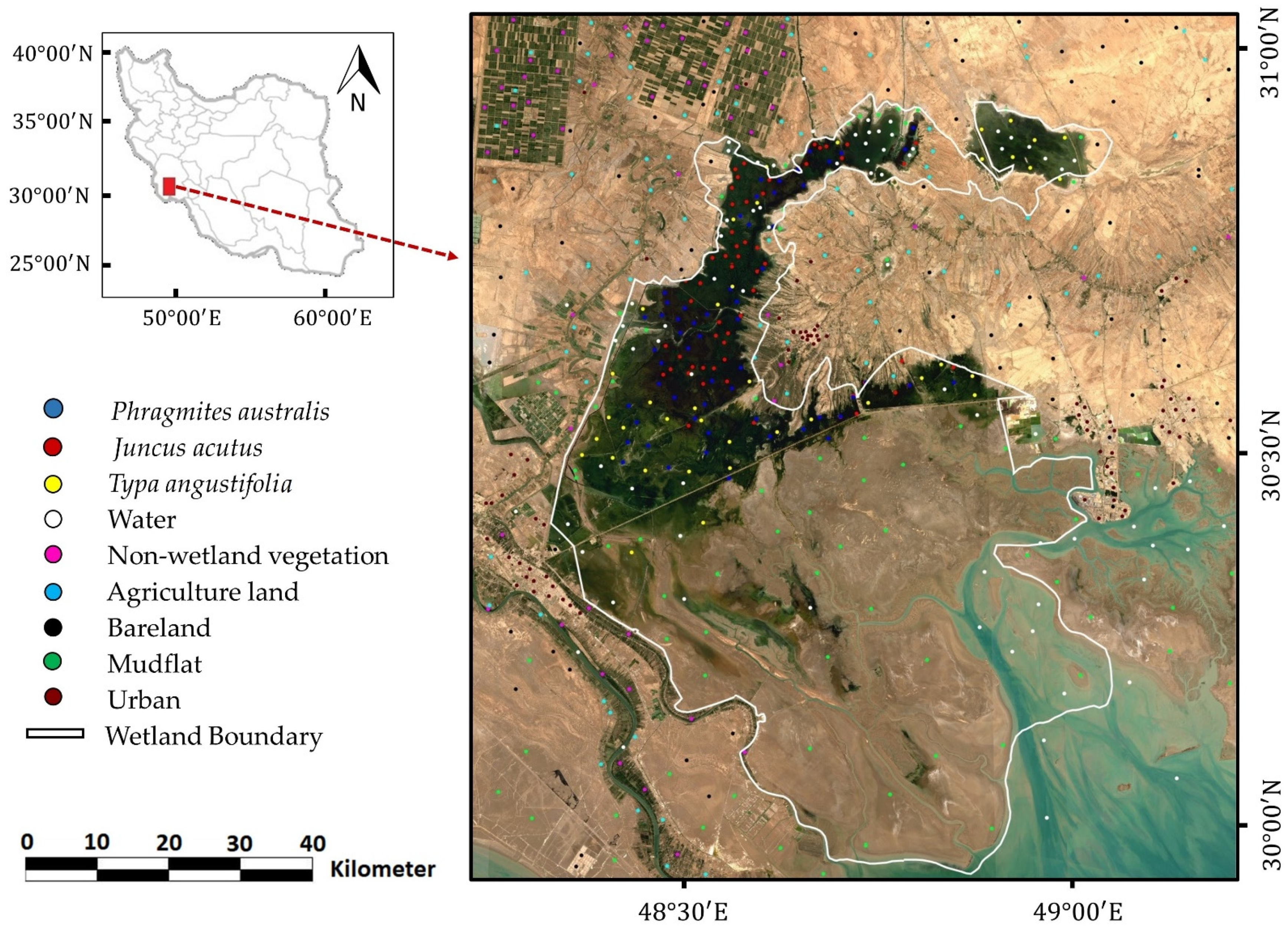
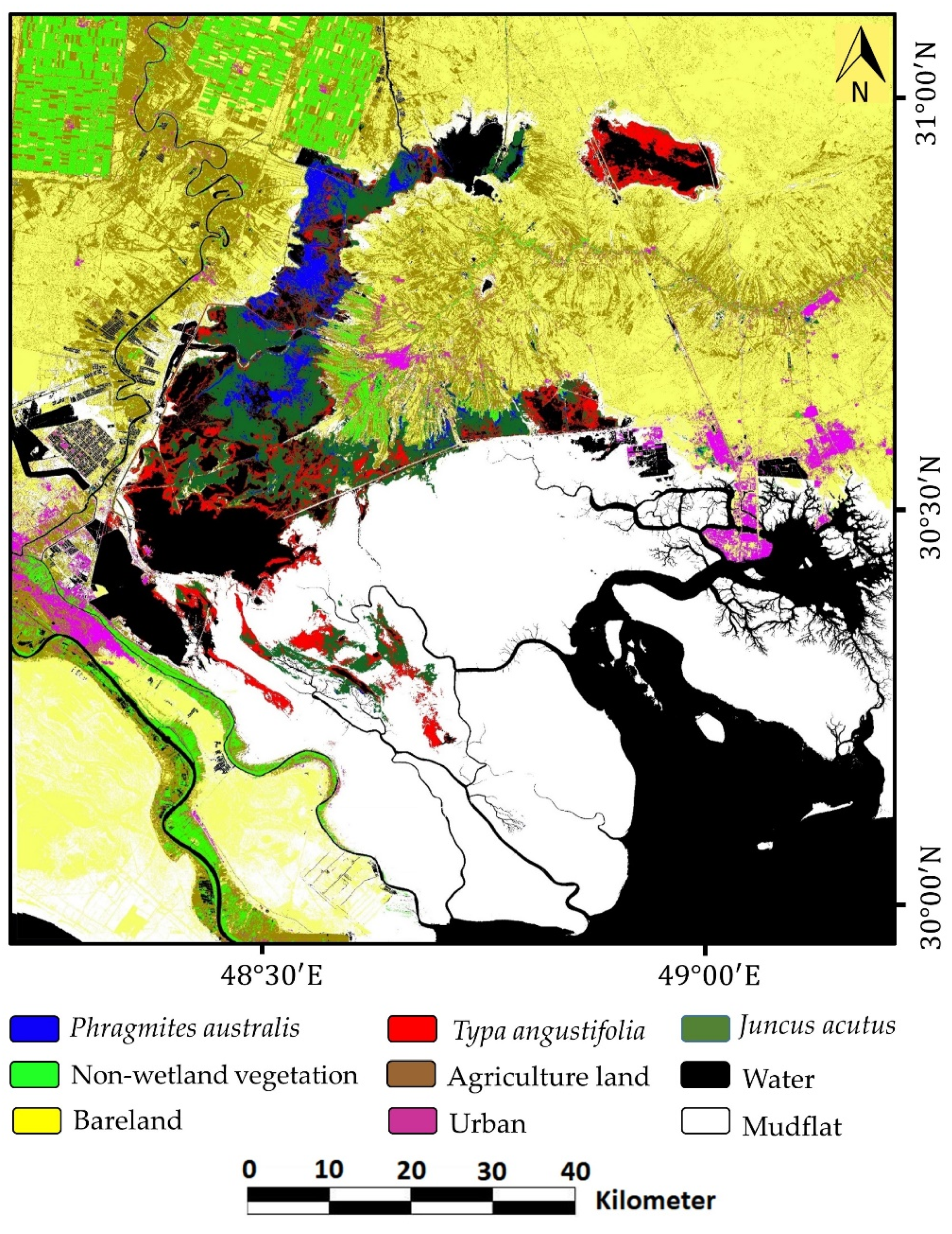
2.1. Study Area

The study area was the ISW and its surrounding regions, located in the province of Khuzestan in southwestern Iran (Figure 1). The ISW covers an approximate area of 537,700 ha (29°30′–31°00′ E and 48°20’–49°10′ N) at the north end of the Persian Gulf and is surrounded by the cities of Abadan, Shadegan, and Mahshahr [58]. It includes a mixture of reed beds, open water, mudflats, and estuaries, as well as small islands and shorelines along the Persian Gulf. It hosts rural populations near the fishery zones, various types of livestock (e.g., buffalo and cattle), and a large number of migratory birds [58]. The ISW consists of three wetlands, including Shadegan, Khor-al-Amaya, and Khor Musa, which play a key role in providing ecological, cultural, and economic opportunities for local residents and acts as a huge barrier against the entry of dust from the deserts of neighboring countries [59]. The ISW is generally divided into a large freshwater marsh, extensive intertidal flats, the Khur Musa Bay and associated islands, as well as the coastal zones of the Persian Gulf. Furthermore, it is mainly fed by both freshwater from the Jarrahi River and tidal influxes of seawater from the Persian Gulf [59], and its predominant plant species include Typa angustifolia, Juncus acutus, Hammada salicornica, and Phragmites australis.

2.2. Field and Reference Data

Visual interpretation of high-resolution images was combined with in situ field visits to collect the required field samples of different wetland classes for the reference year (2020). This was conducted during the wetland’s leaf-on season (1 April 2020–28 June 2020). For this purpose, the initial samples were collected using primary knowledge about the study area for each wetland class by visual interpretation of Google Earth high-resolution data with an appropriate distribution across the study area. Then, field visits were performed to evaluate the accuracy of the collected samples. This step consisted of validation of the visually collected samples using a handheld Garmin Oregon 550 GPS to correct mislabeled samples and to collect complementary samples for each class. A stratified random sampling method was then used to select an equal number of samples for each class to avoid a sample size effect in our classification procedures. Finally, the selected samples were independently divided into the training (70%) and test (30%) sample sets. The distribution of the training sample set across the study area is shown in Figure 1, and more details about both the training and test sample sets are provided in

Table 1. The number and area of the training and test polygons across the study area.

ID	Class Type	Class	Training Samples		Test Samples		Total
			Polygon	Area (Km2)	Polygon	Area (Km2)	Polygon	Area (Km2)
1	Wetland	Juncusacutus	44	7.65	22	3.81	66	11.46
2	Wetland	Typa angustifolia	27	6.2	12	2.4	39	8.6
3	Wetland	Phragmites australis	38	6.92	18	3.53	56	10.45
4	Non-wetland	Non-wetland vegetation	54	12.43	24	6.48	78	18.91
5	Non-wetland	Agriculture land	41	7.51	19	3.73	60	11.24
6	Non-wetland	Water	53	9.3	20	3.12	73	12.42
7	Non-wetland	Bareland	44	12.1	21	6.1	65	18.2
8	Non-wetland	Mudflat	49	11.58	27	6.9	76	18.48
9	Non-wetland	Urban	51	5.72	21	2.43	72	8.15
		Total	401	79.41	184	38.5	585	117.91

. As is clear from Figure 1 and Table 1, three wetland classes along with six non-wetland classes were considered in this study.

2.3. Satellite Dataset

In this study, the time series of Sentinel-1 and Sentinel-2 satellite imageries were employed in GEE for classification and training sample migration. Due to the different characteristics of the wetland components in the study area, including both the ISW and a portion of its surrounding area, a combination of SAR and optical images was applied to obtain accurate classification maps [13,21,22,23,24].

Table 2. The number of images and acquisition dates of Sentinel-1 and Sentinel-2 time series.

Year	Number of Images		Total	Acquisition Date
	Sentinel-1	Sentinel-2
2018 (Target)	114	119	233	1 April 2018–29 June 2018
2019 (Target)	120	110	230	1 April 2019–29 June 2019
2020 (Reference)	112	111	223	1 April 2020–29 June 2020
2021 (Target)	120	97	217	1 April 2021–29 June 2021

provides basic information about the Sentinel-1 and Sentinel-2 time series images that were used in this study. More details are provided in the following two subsections.

2.3.1. Sentinel-1 Data

The Sentinel-1 mission, launched on April 2014 by the European Space Agency (ESA), consists of the Sentinel-1A and Sentinel-1B satellites. The satellites survey the entire world with a 6-day temporal resolution. They provide dual-polarization (VV and VH) C-band Synthetic Aperture Radar (SAR) data with a 10-m spatial resolution in both ascending and descending modes [60,61].

Due to the specific characteristics of SAR images, Sentinel-1 data have been widely employed in wetland mapping [9,13,20]. In this study, four time series of Sentinel-1 imageries with a 10-m spatial resolution in both ascending and descending modes with a combination of the VV and VH polarizations were employed in GEE. These images were captured in the ISW’s growing season (1 April to 30 June) for the reference year (2020) and target years (2018, 2019, and 2021).

2.3.2. Sentinel-2 Data

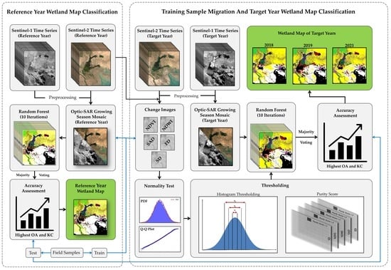
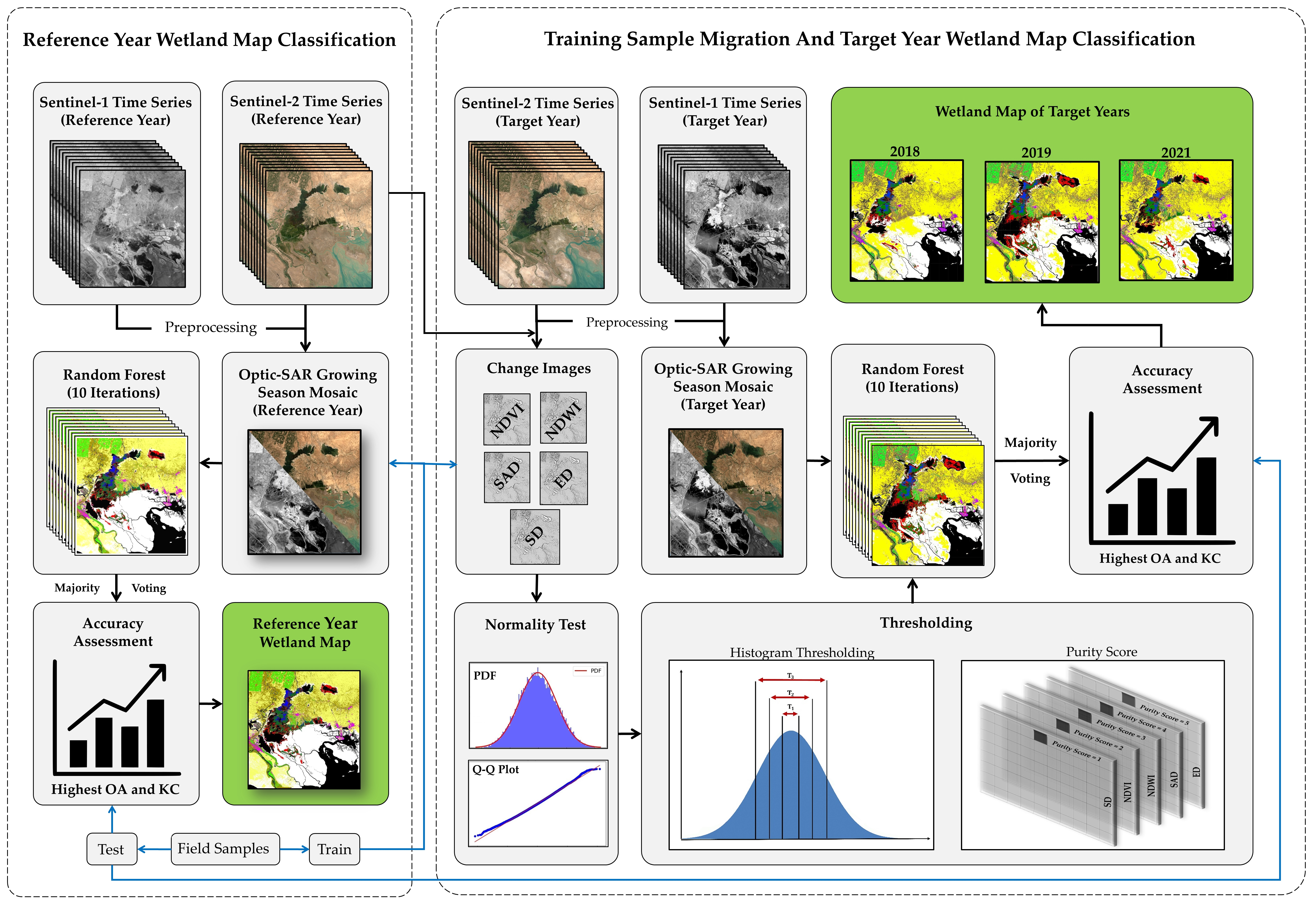
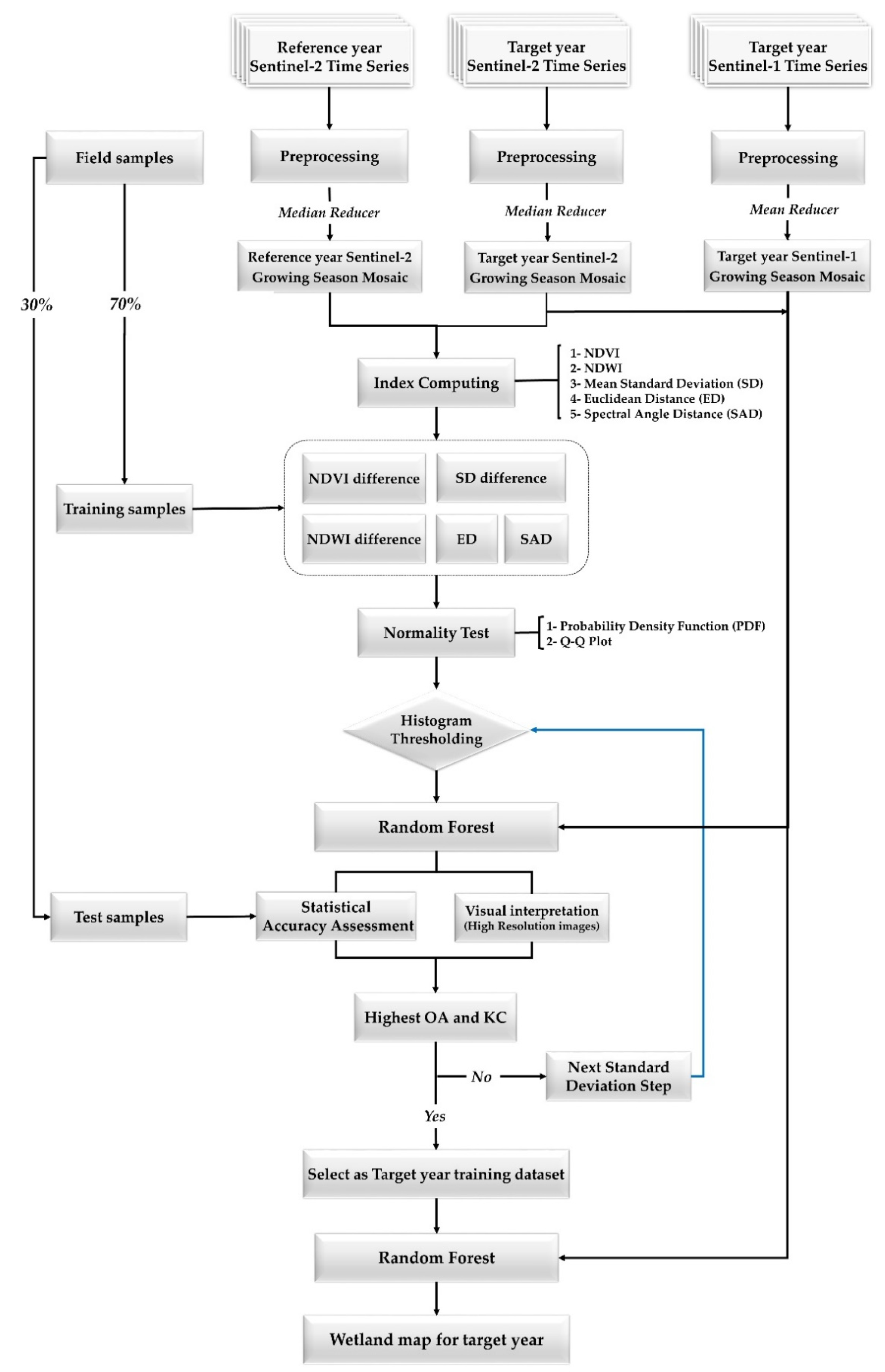
The Sentinel-2 satellites were launched by the ESA on June 2015 and March 2017, respectively. Both the Level-1C (L-1C) Top-of-Atmosphere (ToA) reflectance, and Level-2A (L-2A) Surface Reflectance (SR) are available in GEE. L-1C and L-2A data contain 13 and 12 spectral bands (e.g., visible, Near Infrared (NIR), Red Edge (RE), and Shortwave Infrared (SWIR)), respectively, with 10-, 20-, and 60-m spatial resolutions [61]. In addition to a high spatial resolution, the presence of three RE bands in Sentinel-2 data is very helpful in wetland classification [23].

In this study, due to computation efficiency, all available bands were analyzed throughout a feature selection method [62], and only 6 important bands were selected: 4 bands with a 10-m resolution (B2, B3, B4, and B8) and 2 RE and SWIR bands with a 20-m resolution. Similar to the Sentinel-1 dataset, four Sentinel-2 time series were generated for the reference year, and each of the target years using all available images in the growing season.

3. Methodology

This section describes a two-phase work flow, including (1) generating the nine-class wetland map of the reference year (2020), consisting of satellite data preprocessing, reference year wetland map classification, and accuracy assessment (Section 3.1), and (2) carrying out a novel automatic method for migrating training samples to each target year and their following classification work flow, consisting of a methodology for training sample migration and its accuracy assessment as well as the target years’ wetland map classification (Section 3.2).

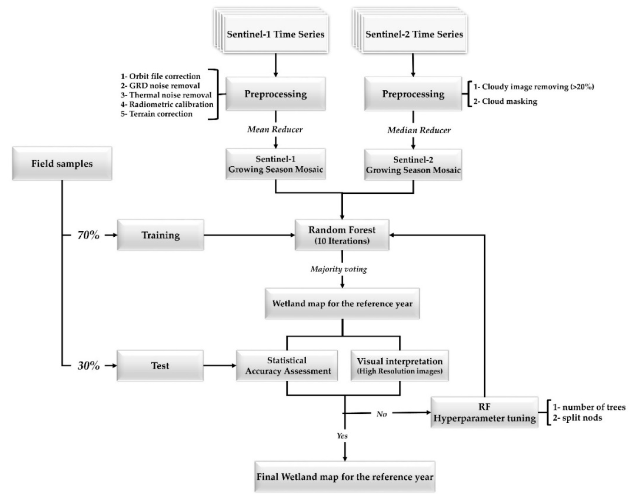
3.1. Reference Year Wetland Classification

Figure 2 demonstrates the workflow of the developed method for generating a wetland map of the ISW with a 10-m spatial resolution using Sentinel images and the Random Forest (RF) classifier within the GEE cloud computing platform. The steps shown in the flowchart are detailed in the following two subsections.

3.1.1. Satellite Data Preprocessing

GEE offers ready-to-use products, and consequently, the necessary preprocessing steps had already been applied to the Sentinel data [26,27]. GEE’s Sentinel-1 data collection provided C-band SAR data that were initially preprocessed by the five following steps: (1) applying orbit file correction, (2) GRD border noise removal, (3) thermal noise removal, (4) radiometric calibration, and (5) terrain correction [26,27]. However, despite the GEE’s initial preprocessing, the Sentinel-1 scenes included speckle noise (also known as salt and pepper noise), which has a negative impact on the classification results [15,20,63]. Thus, a mean filter with a $3\times 3$ moving window was applied to Sentinel-1 scenes to reduce the speckle noise. Finally, a mean reducer function was applied to all available scenes in each time series to generate four single growing season mosaics. In fact, each pixel was assigned to its mean value throughout the entire growing season, which resulted in a seasonal mosaic that was less affected by image acquisition conditions [24,41].

Sentinel-2 datasets also required a few preprocessing steps before being utilized in classification. In this study, the following preprocessing steps were applied to Sentinel-2 images: (1) excluding images with more than 20 percent cloud cover from each time series; (2) applying a cloud mask algorithm to all available scenes in each time series; and (3) applying a median reducer function to all available scenes in each time series, in which each pixel was assigned to its median value throughout the entire growing season. This step resulted in a cloud-free seasonal mosaic in addition to noise removal [24,41].

After preprocessing of both the Sentinel-1 and Sentinel-2 datasets, a single mosaic image that included all the multispectral and SAR mosaics was generated. This mosaic image was fed to the RF algorithm to produce the wetland map of the reference year.

3.1.2. Classification

Among the common supervised machine learning algorithms, RF has proven to be more efficient for wetland mapping [13,24,28,32]. RF is an ensemble learning model and includes a large number of decision trees that are independently built and trained by different numbers of variables and samples [24,28,32]. Each tree then individually assigns a class to each pixel, and eventually, the final decision for each pixel is conducted through a bootstrap aggregation procedure [21,24]. The most important advantages of the RF algorithm are (1) its compatibility with multi-source and multi-dimensional datasets (e.g., the synergy of multispectral and SAR datasets); (2) being less affected by noise; and (3) high performance and robustness. RF has two main hyper parameters: the number of decision trees and the number of splitting nodes [24,41].

In this study, an RF classifier was implemented in GEE to generate the wetland map of the reference year. Through a trial-and-error procedure, the optimal number of trees (500) was selected by means of an iterative accuracy assessment, where the highest classification accuracy using the test samples was obtained. The classification was iterated 10 times with different sets of test and training samples to minimize the probability of misclassified pixels, and the final classes were assigned through majority voting.

Finally, both the visual interpretation of high-resolution Google Earth images and statistical assessment by analyzing the confusion matrix of the classification were used for validation. Using the confusion matrix, the accuracy indices of the OA, KC, producer’s (PA) and user’s (UA) accuracies were calculated.

3.2. Automatic Wetland Classification for Target Years Using Migrated Samples

Inspired by studies conducted on reference sample migration [40,41,42,43], we proposed a novel method for generating wetland maps for the target years of 2018, 2019, and 2021 (see Figure 3).

The proposed method had five main steps: (1) three indices, including the NDVI, NDWI, and the mean Standard Deviation (SD) of the Sentinel-2 spectral bands were calculated for the multispectral mosaics of both the reference and target years; (2) three computed indices for the reference year were then subtracted from those of the target years, resulting in three change images for each pair of reference–target years; (3) in addition to the abovementioned indices, ED and SAD similarity measures were also calculated for each pair of reference–target years to result in five change images for each pair. These five difference images were the indicators of change between the reference and target samples in terms of the vegetation content (NDVI difference), water content (NDWI difference), texture (SD difference), magnitude of change (ED), and direction of change (SAD); (4) a histogram-based method was applied to determine the optimum threshold for unchanged pixels in each target year; and (5) a wetland map for the three target years was generated using the samples migrated from step 4. More details of the proposed migration method are provided in the following subsections.

3.2.1. Input Indices for the Migration Algorithm

Five indices were calculated and compared to migrate the high-quality unchanged training samples from the reference year to each target year. These indices are described below.

The NDVI (Equation (1)) and NDWI (Equation (2)) have been widely used for vegetation and water mapping, respectively [26,49,64,65,66,67,68]:

$$NDVI=\frac{NIR-RED}{NIR+RED}$$

(1)

$$NDWI=\frac{Green-NIR}{Green+NIR}$$

(2)

The SD (Equation (3)) defines the dispersal of data from the mean, which is used in image processing to extract first-order textural measures [69]. The mean SD of the Sentinel-2 spectral bands was used to generate texture images from multispectral growing season mosaics of the reference and target years. A $3\times 3$ moving window was applied to calculate the SD across the images. For each multispectral mosaic, this was performed for all the spectral bands, and finally, each pixel was assigned by its mean SD using a mean reducer:

$$\sigma =\sqrt{{\frac{{{\displaystyle \sum }}_{i=1}^9\left(X_i-\overline{X}\right)}{N}}^2}$$

(3)

where $\sigma$ is the Standard Deviation; $i$ is the pixel index; $X_i$ is the spectra of the ith pixel; and $\overline{X}$ is the mean of all pixel values in the defined window.

The ED (Equation (4)) and SAD (Equation (5)) were also calculated as similarity indices to present the magnitude and direction of change between the reference and target spectra [70]:

$$ED=\sqrt{{{\displaystyle \sum }}_{i=1}^N(A_{i\left(t1\right)}-B_{i\left(t2\right)}})$$

(4)

where ED is the Euclidean Distance; $A$ is the reference spectra in time $t1$; $B$ is the target spectra in time $t2$; $i$ is the index of the band; and $N$ is the number of bands. The ED values range between 0 and 1. The ED value will be 0 if both the reference and target spectra are identical:

$$\begin{gathered} \theta ={\cos }^{-1}\frac{{{\displaystyle \sum }}_{i=1}^N{A}_{i\left(t1\right)}{B}_{i\left(t2\right)}}{\sqrt{{{\displaystyle \sum }}_{i=1}^N{(A_{i\left(t1\right)})}^2{{\displaystyle \sum }}_{i=1}^N{(B_{i\left(t1\right)})}^2}} \\ SAD=\cos \left(\theta \right) \end{gathered}$$

(5)

where $\theta$ is the spectral angle; $A$ is the reference spectra in time $t1$; $B$ is the target spectra in time $t2$; $i$ is the index of the band; and $N$ is the number of bands. The SAD ranges between 0 and 1. The SAD value will be 1 if both the reference and target spectra are identical. It should be noted that although ED and SAD indicate the magnitude and direction of change, the change images in the other applied indices (i.e., NDVI, NDWI, and SD) were computed by subtracting their values in each pair of reference–target years.

In summary, five change images for each pair of reference–target years were computed using the five indices. Afterward, the corresponding pixel values of the training samples were extracted to identify their unchanged training samples through the procedure described in the following subsection.

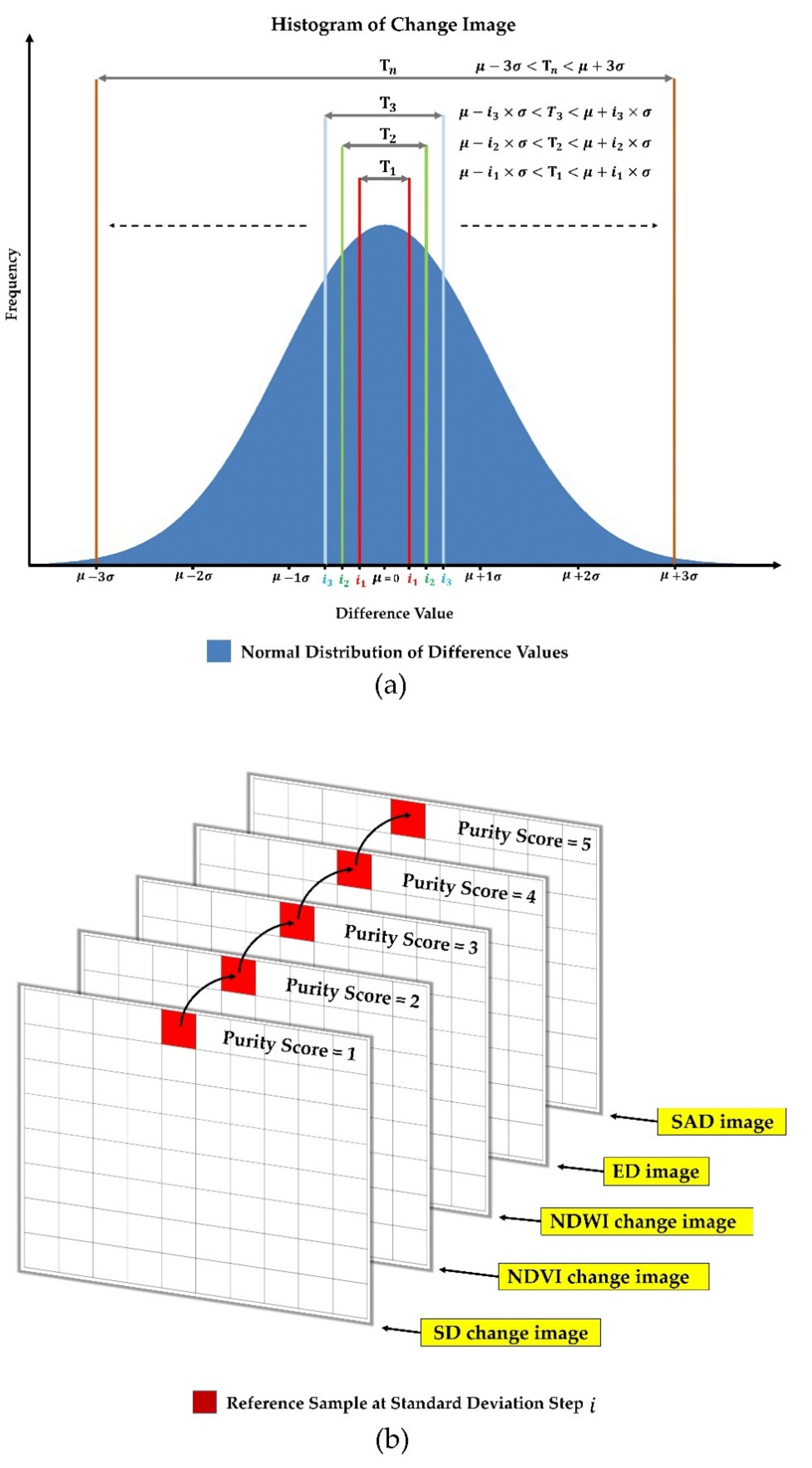
3.2.2. Determination of the Optimum Threshold for Selecting Unchanged Training Samples

In order to identify unchanged samples, an optimum threshold was determined for each target year using a histogram-based method. Selecting the optimum threshold value, one of the most important steps in change detection procedures, directly affects the results [13,53,54]. Various methods have been developed for determining the thresholds [13,53,54]. Of these methods, histogram thresholding is one of the simplest and most widely used methods [55,56,57]. However, prior knowledge about the behavior of the dataset utilized is required for this method [33]. The shape of a histogram varies depending on the distribution of data (e.g., normally distributed data with a unimodal histogram and symmetric around the mean) [55]. In unimodal histograms, different threshold determination methods are required. Image differencing is a method in which two temporal scenes are subtracted from each other, resulting in a change image in which pixel values indicate the rate of change [37,38,39]. Consequently, the most likely unchanged pixels are distributed around zero. If the change image values are normally distributed, the most likely unchanged pixels are associated with values close to zero at each side of the mean value. Identifying the most likely unchanged pixels in such histograms is challenging because they can be distributed at any SD of the mean. Moreover, it can be even more difficult when the change is investigated from different aspects (e.g., spectral and structural characteristics), in which multiple change images are simultaneously considered for change detection. In this context, one solution is to gradually select equal proportions of pixels in each change image at each side of their mean using a stepwise value and evaluate the quality of the selected unchanged pixels at each step by using statistical tests (see Figure 4a). Additionally, in order to ensure only the most likely unchanged pixels are selected at each step, they can be given a purity score based on the frequency of their presence among change images, indicating the number of their characteristics that remained unchanged. In this case, the most suitable pixels were those with the highest purity score. Therefore, they were selected at each step (Figure 4b). This process continued until no further improvement in accuracy was observed. Thus, the last step with the highest accuracy was selected as the threshold value. Since SD indicates the distance from the mean value, the ascending confidents of SD were used as the step values through Equation (6):

$$\mu -a_i\times \sigma <{\mathrm{T}}_i<\mu +a_i\times \sigma$$

(6)

where $i$ is the step index; $\mu$ is the mean value;$\sigma$ is the SD;$a_i$ is the ith step; and ${\mathrm{T}}_i$ is the threshold in the step index $i$.

In this study, the most likely unchanged training samples were selected for each target year using the abovementioned strategy. Therefore, the histogram of five change images was created for each target year, followed by the graphical normality tests. It is worth noting that the statistical normality tests were ignored, since an approximately normal distribution also satisfied the requirements of this method. The graphical normality tests included (1) plotting the Probability Density Function (PDF) curve of change images fitted to their histograms and (2) analyzing their Quantile-Quantile (Q-Q) plots. In the first graphical normality test, the PDF of the random values in each change image was plotted to determine their distribution and then fitted to their histogram to ensure they were normally distributed (a bell-shaped PDF curve). In the second graphical normality test, the Q-Q plot was applied to test the normality among change images. Here, the values related to each change image were plotted against a predefined normal dataset in a Q-Q plot. Following the above two graphical normality tests, change detection was performed for each target year as follows:

• The corresponding pixel values of the training samples in the reference year image were independently extracted from each of the five change images, resulting in five sets of pixels.
• For each set, the mean and SD were independently computed.
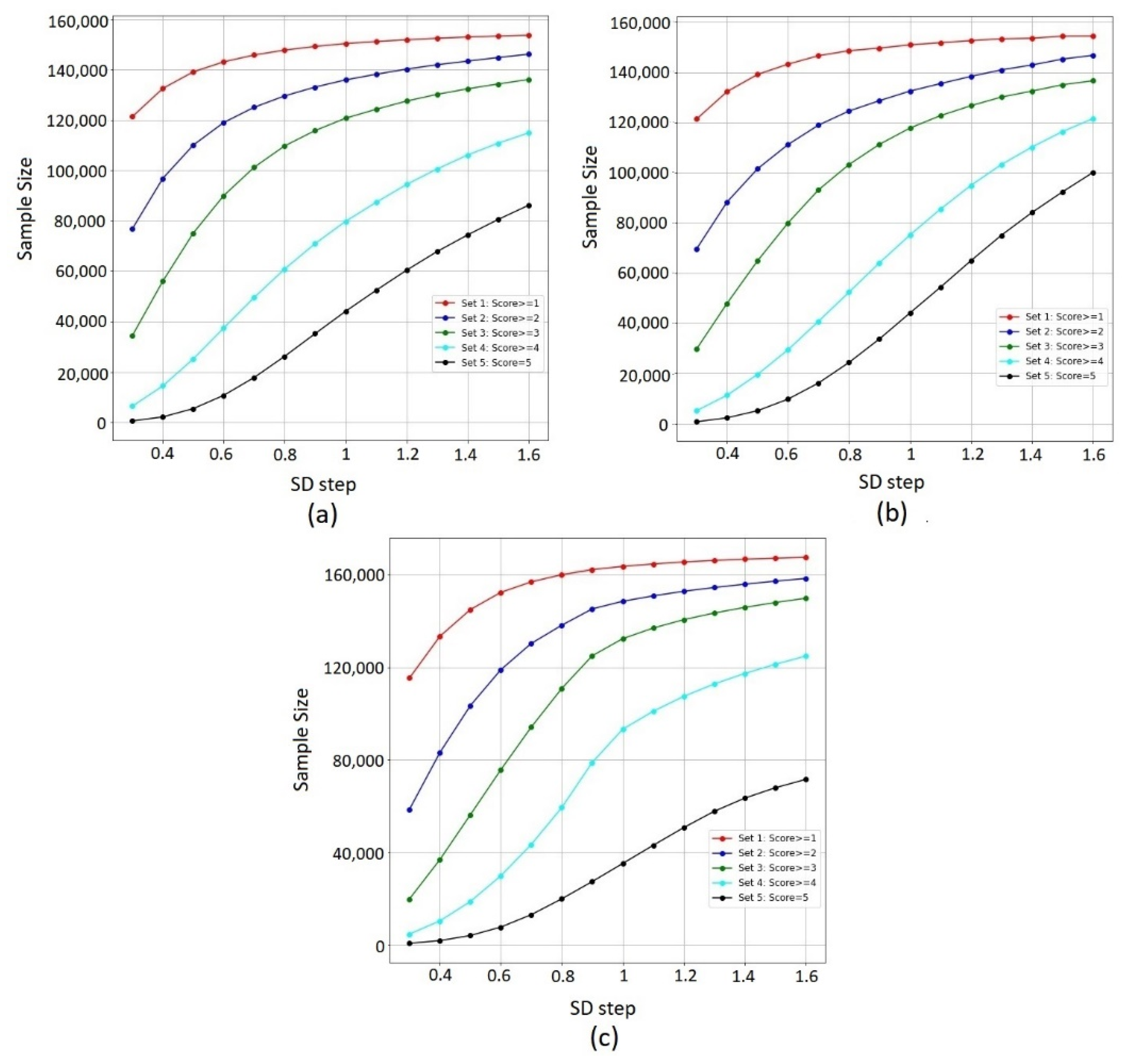
• A stepwise procedure was performed to extract the potentially unchanged pixels at each step from each set of pixels (see Figure 4a).
• At each step, pixels were given a purity score between 1 and 5 based on the frequency of their presence among five sets. A score of 1 indicated that the pixel existed only in one set (i.e., only one of the five purity conditions was satisfied, and the pixel was potentially changed), and a score of 5 indicated that the pixels existed in all five sets (i.e., all five purity conditions were satisfied, and the pixels were likely unchanged). Thus, the pixels with a score of 5 were selected at each step (see Figure 4b).
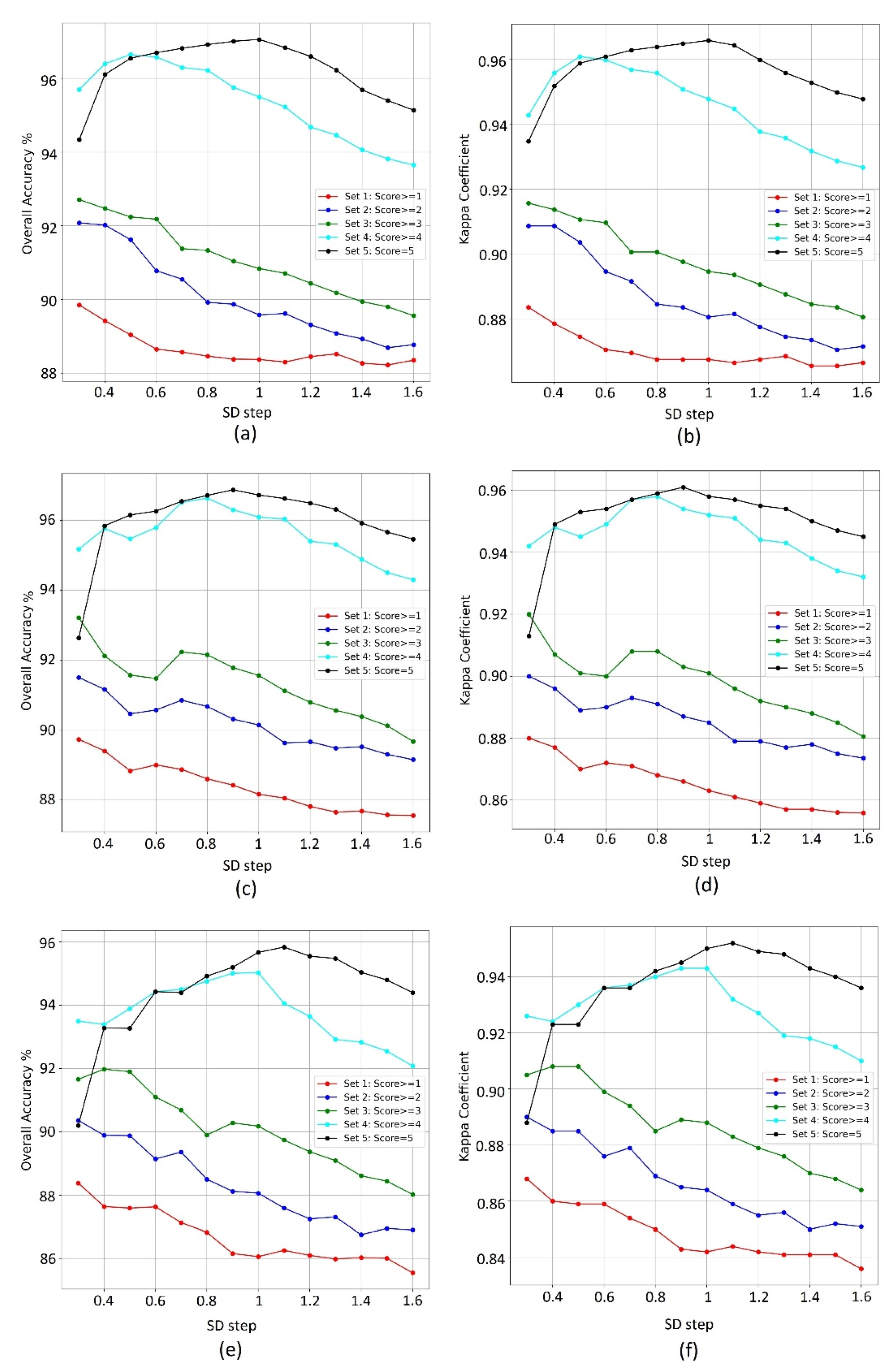
• The unchanged pixels selected at each step were then used to classify the test samples that were specified in Section 2.2, and the quality of these unchanged pixels was evaluated using the OA and KC values derived from the confusion matrix of the classification.
• Steps 4 and 5 were repeated until no further improvement in classification accuracy was achieved, and the abovementioned statistics (i.e., the OA and KC) began to decline. In this case, the step with the highest accuracy was selected as the optimal threshold value.

Steps 1–6 were performed to select unchanged samples for all the target years. After the unchanged training samples had been selected for each target year, they were applied to classify the wetland maps of the target years. More details about selecting the optimal threshold value are provided in the Results section (Section 4.2.2).

4. Results

4.1. Wetland Classification for the Reference Year

Figure 5 represents the generated wetland map of the study area for the reference year of 2020. Visual inspection of the generated map showed the high performance of the proposed method in delineating different wetland and non-wetland classes. For example, different components of the ISW ecosystem, including water bodies, three main vegetation types (i.e., Juncus acutus, Typa angustifolia, and Phragmites australis), and a significant area of mudflats, were successfully isolated from their surrounding LCs. The results also indicated high performance in the delineation of water bodies all over the study area. Another strength of the method was the successful delineation of the agriculture land class across the study area. For the non-wetland vegetation class, good performance was also observed across the study area, especially for the vegetation located in the northwestern part of the study area. However, multiple misclassifications were observed among adjacent wetland and non-wetland vegetation types, such as those among Juncus acutus, Typa angustifolia, and the non-wetland vegetation classes. Additionally, visual inspection showed reasonable performance in classifying urban areas. However, occasional misclassifications between the urban and bareland classes were observed.

The statistical accuracy assessment of the wetland map of the reference year also showed promising results for all wetland and non-wetland classes (

Table 3. Confusion matrix of the wetland map of the reference year (2020).

	Juncus acutus	Typa angustifolia	Phragmites australis	Water	Non-Wetland Vegetation	Agriculture Land	Bareland	Mudflat	Urban
Juncusacutus	7352	14	0	0	196	12	0	0	0
Typa angustifolia	43	7311	152	0	0	1	0	0	0
Phragmites australis	0	129	7221	0	16	0	0	0	0
Water	0	0	0	7605	0	0	0	11	0
Non-wetland vegetation	152	1	0	0	7420	21	0	0	0
Agriculture land	1	9	0	0	11	7473	53	0	21
Bareland	0	0	0	0	0	98	7466	9	108
Mudflat	0	0	6	13	0	3	23	7555	31
Urban	0	1	5	0	2	68	131	64	7208
PA%	97.07	97.39	98.03	99.86	97.71	98.74	97.20	99	96.38
UA%	97.4	97.94	97.79	99.83	97.06	97.36	97.3	98.9	97.83
	OA = 97.93%, KC = 0.97

). The OA and KC were very high, reaching 97.93% and 0.97, respectively. Moreover, a closer look at the confusion matrix revealed high class-specific accuracies (i.e., PA and UA), with the highest accuracy achieved for the water class. However, upon confirming visual inspection, occasional misclassifications were observed among the wetland and non-wetland classes. For example, wetland vegetations (i.e., Juncus acutus, Typa angustifolia, and Phragmites australis) were generally classified with high accuracy; however, some misclassifications occurred, mainly among Juncus acutus, Typa angustifolia, and the non-wetland vegetation class, as well as between Typa angustifolia and Phragmites australis. The bareland and urban classes also obtained high classification accuracies, yet they were slightly confused.

4.2. Migration of Training Samples

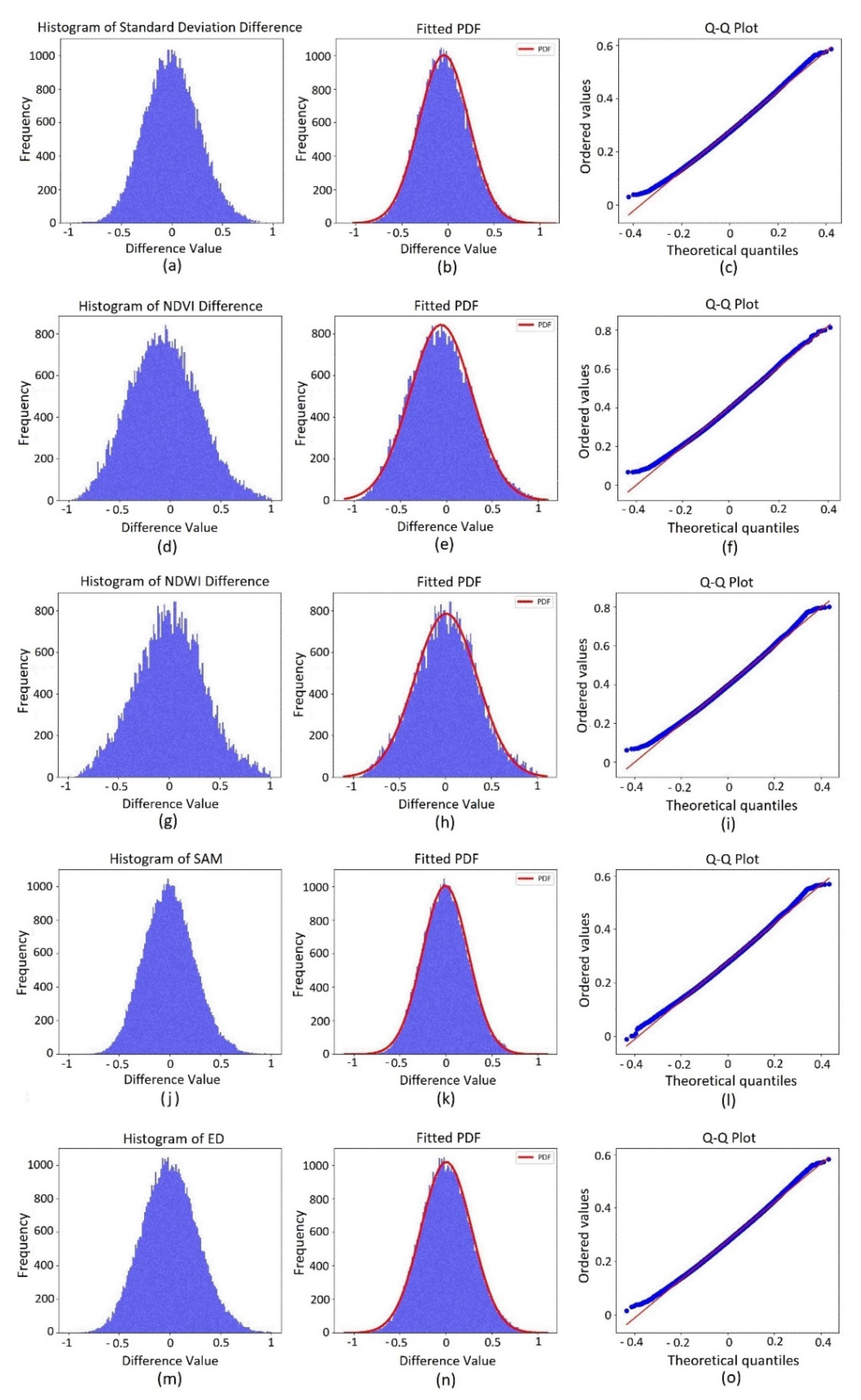
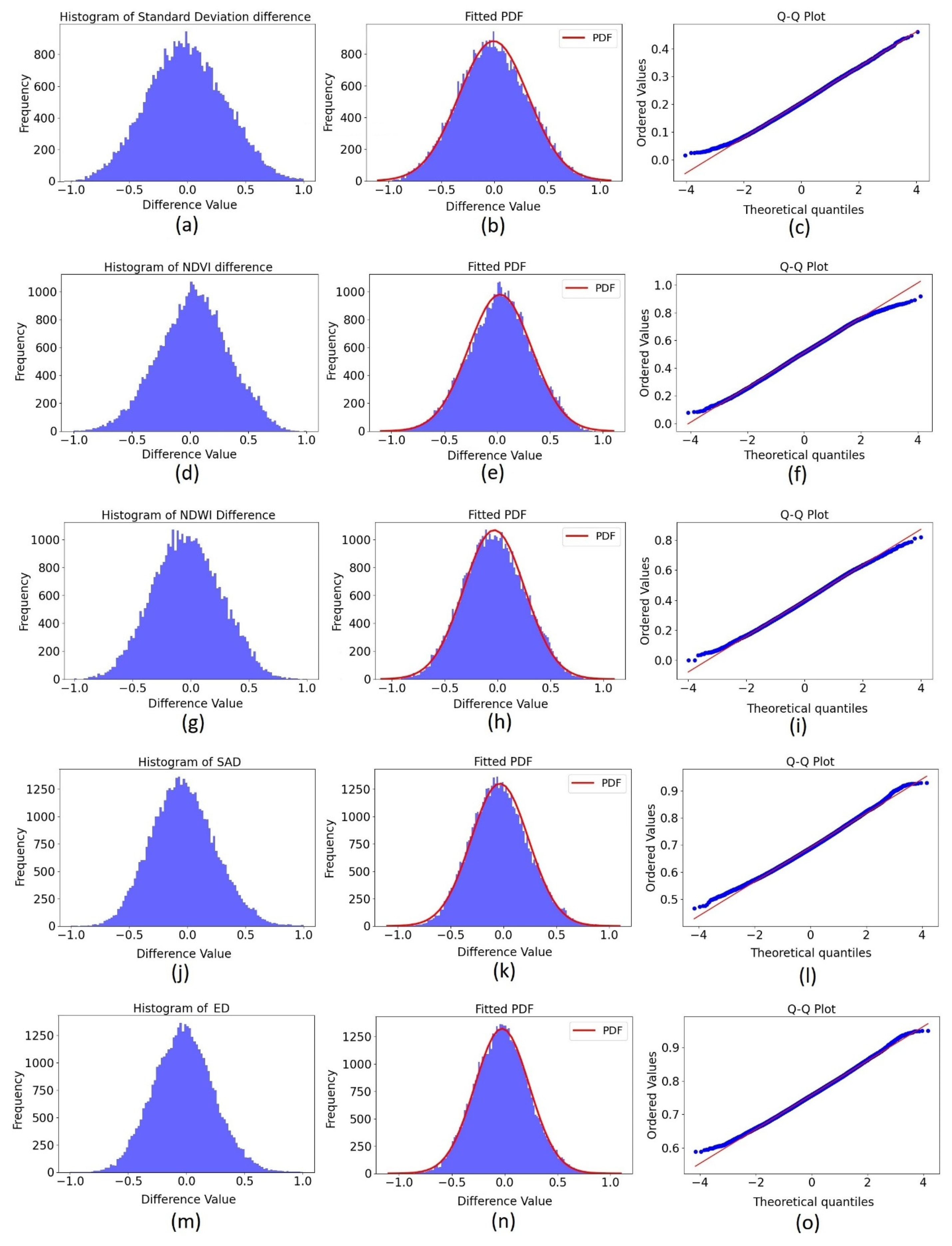
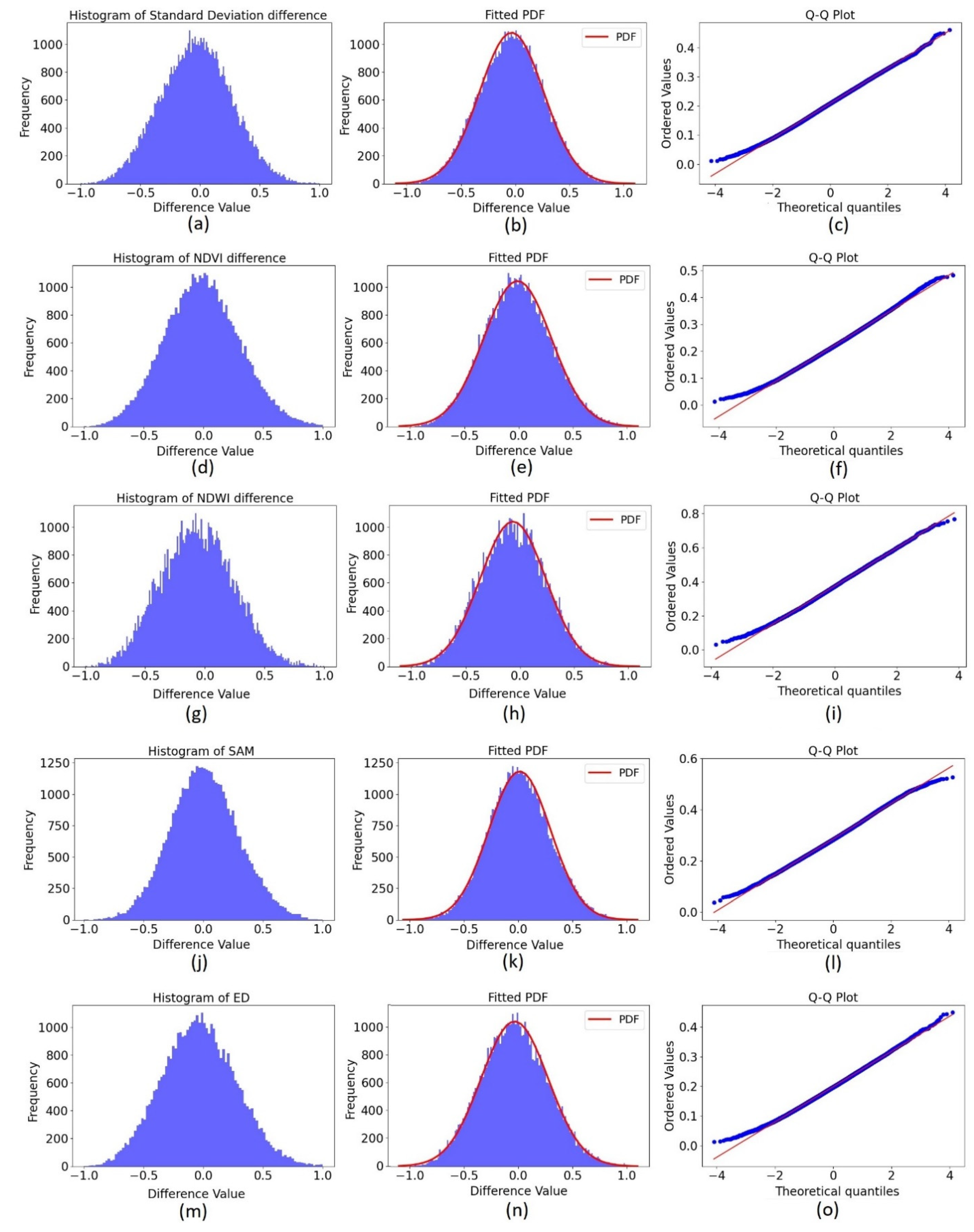
4.2.1. Normality Test

As mentioned in Section 3.2.2, before selecting the optimum threshold value for change analysis, it is important to check if the PDF of the pixel values follows a normal distribution (Figure 6).

Therefore, the PDF of random values in each change image was first investigated and then fitted to their histogram (Figure 6a,d,g,j,m), confirming their normality (a bell-shaped PDF curve). For instance, the results of the target year of 2021 are illustrated in Figure 6b,e,h,k,n (see Appendix A Figure A1 and Figure A2 for the results of the target years of 2019 and 2018). Moreover, the Q-Q plot (i.e., the second method for normality) showed an almost straight line for all change images (see Figure 6c,f,i,l,o). A slight and negligible distortion was observed for the NDVI and NDWI Q-Q plots, indicated by the slightly longer right tails observed in their histograms.

4.2.2. Optimum Threshold Determination

Figure 7 demonstrates the procedure for determining the optimum threshold value for the target years of 2021 (Figure 7a,b), 2019 (Figure 7c,d), and 2018 (Figure 7e,f) based on the steps described in Section 3.2.2.

Here, the samples were categorized into five sets based on their purity scores, including the samples purity scores ≥1, ≥2, ≥3, ≥4, and =5. The SD steps began from 0.3, since for some classes, there were no samples with purity scores of 5 at 0.1 and 0.2 SD (Figure 7). The rate of increase or decrease of the OAs and KCs at each step for five sets of samples in all target years can be observed in Figure 7. Similar behavior was observed corresponding to each target year. For example, sets 1, 2, and 3 showed a decreasing rate of OAs and KCs from the beginning as the SD steps increased, whereas sets 4 and 5 began with an increasing rate of OAs and KCs, which then gradually declined at a certain SD step (i.e., the optimum threshold value). Between sets 4 and 5, set 4 started to decline earlier, and its highest OA and KC were also lower than those of set 5. Regarding sets 1, 2, and 3, set 3 (i.e., with a purity score of 3) obtained the highest average classification accuracy in all target years. Between sets 1 and 2, set 2 achieved higher accuracies, and set 1 had the poorest performance among all sets, obtaining the lowest OA and KC values in all target years. In general, sets 1–3 showed similar performance among the target years, except for the higher average OA and KC obtained in 2021 (see Figure 7a,b), and approximately similar results were observed in the OA and KC in each target year.

In terms of sets 4 and 5, they obtained lower classification accuracy in the beginning compared with the later steps and then continued to obtain higher accuracies up to a certain step (i.e., the optimum threshold value), after which they declined. As shown in Figure 7a,b, corresponding to the target year of 2021, sets 4 and 5 reached OAs of 95.87% and 94.31% and KCs of 0.94 and 0.93 at their first SD step, respectively. Then, both continued to achieve higher accuracies until step 0.6, where both sets obtained almost similar accuracies. Afterward, the accuracy of set 4 started to decrease, while set 5 kept obtaining higher accuracies until step 1.0, where the highest OA and KC were achieved. In other words, the samples from 2021 with a purity score of 5 that were distributed at 1 SD value in all change images were capable of classifying the test samples with an OA and KC of 97.06% and 0.96, respectively. This SD step was, in fact, the optimum threshold value required to select the high potentially unchanged samples from the target year of 2021.

A similar procedure was applied for the target years of 2018 and 2019, as presented in Figure 7. For year 2018 (Figure 7e,f), the optimum threshold was determined at 1.1, by which point an OA and KC of 95.89% and 0.95 were achieved, respectively. For 2019 (Figure 7c,d), the optimum threshold value was determined at 0.9, by which point an OA and KC of 96.83% and 0.96 were obtained in classifying the test samples, respectively. These results indicated that the most likely unchanged samples were distributed almost at one SD from the mean value in the change images.

Figure 8 shows the relationship between the SD step and sample size corresponding to each of the five sets in the target years of (a) 2021, (b) 2019, and (c) 2018. They suggest a direct relationship between the SD steps and the sample size. Increases in the rate of the sample size in sets 1, 2, and 3 (and slightly in set 4) were considerably greater than those in set 5 in all target years. In fact, sets 1, 2, and 3 had a logarithmic growth rate in the sample size, while an almost exponential growth rate was observed for set 1 in all target years. For example, Figure 8a shows the increasing rate of the sample size for the target year of 2021. Regarding sets 1–3, a collection of 121,342, 78,835, and 37,439 samples was selected in the first step, respectively, while only 6437 and 710 samples were selected for sets 4 and 5 at the first SD step, respectively. Furthermore, the sample size of set 1 at the threshold value corresponding to each target year was much lower than those in the other sets (Figure 8).

4.3. Wetland Classification for the Target Years

The second aim of this study was to generate wetland maps for the target years of 2018, 2019, and 2021, for which no training samples were available, by migrating the reference year’s training samples to these years using the proposed training sample migration method. As explained in detail in Section 4.2.2, this was performed by determining the optimum threshold for unchanged samples using a histogram thresholding method with respect to the purity scores of the migrated samples.

The analyses performed for selecting the optimum threshold values for the unchanged training samples (e.g., Figure 7 and Figure 8) resulted in identifying the number of the most likely unchanged training samples as well as the accuracy levels for the target years (see

Table 4. Summary of the results in migrating reference samples to each target year using the proposed method.

Year	Optimum Threshold (SD)	Migrated Samples	OA%	KC	Purity Score
2021	1	44,078	97.06	0.96	5
2019	0.9	38,762	96.83	0.96	5
2018	1.1	43,146	95.89	0.95	5

). For example, the highest classification accuracy for the target year of 2021 was obtained during the SD step of 1 (Figure 7a,b), in which 44,078 samples (migrated samples) with a purity score of 5 were selected as unchanged samples between this year and the reference year of 2020 (Figure 8a). In terms of the target years of 2018 (Figure 7e,f) and 2019 (Figure 7c,d), 43,146 (Figure 8c) and 38,762 (Figure 8b) samples were migrated, respectively (see Table 4).

These samples were then used to generate wetland maps for the target years of 2018, 2019, and 2021 (see Appendix A, Figure A3, Figure A4 and Figure A5). To evaluate the accuracy of the samples migrated to each target year, they were applied to classify the test sample set. The confusion matrices of the target years’ wetland maps using the 2020’s test sample set are presented in

Table 5. The confusion matrices of the target years of (a) 2021, (b) 2019, and (c) 2018 using the samples migrated from reference year 2020.

	Juncus acutus	Typa angustifolia	Phragmites australis	Water	Non-Wetland Vegetation	Agriculture Land	Bareland	Mudflat	Urban
Juncus acutus	7177	109	0	0	250	38	0	0	0
Typa angustifolia	192	7146	164	0	0	3	0	2	0
Phragmites australis	0	135	7121	0	67	0	0	43	0
Water	0	0	0	7598	0	0	0	18	0
Non-wetland vegetation	153	5	41	0	7318	77	0	0	0
Agriculture land	4	34	0	0	21	7464	3	27	15
Bareland	0	0	0	0	0	2	7445	114	128
Mudflat	0	1	68	4	0	0	38	7520	0
Urban	0	0	4	0	2	69	169	11	7267
PA%	94.76	95.19	96.67	99.76	97.16	98.63	96.93	98.55	96.59
UA%	95.36	96.18	96.26	99.95	95.24	97.53	97.26	97.22	98.17
	OA = 97.06%, KC = 0.96
(a)
	Juncus acutus	Typa angustifolia	Phragmites australis	Water	Non-Wetland Vegetation	Agriculture Land	Bareland	Mudflat	Urban
Juncus acutus	7192	121	0	0	253	8	0	0	0
Typa angustifolia	196	7042	248	0	10	10	0	0	1
Phragmites australis	0	329	7007	0	0	1	0	28	1
Water	0	0	2	7609	0	0	0	5	0
Non-wetland vegetation	213	1	0	0	7327	53	0	0	0
Agriculture land	0	9	0	0	31	7477	0	5	46
Bareland	0	0	0	0	0	16	7461	41	163
Mudflat	0	1	10	2	0	10	41	7545	22
Urban	0	0	5	0	1	67	172	39	7195
PA%	94.96	93.81	95.13	99.91	96.48	98.8	97.14	98.87	96.2
UA%	94.62	93.86	96.36	99.97	96.13	97.84	97.22	98.46	96.86
	OA = 96.83%, KC = 0.96
(b)
	Juncus acutus	Typa angustifolia	Phragmites australis	Water	Non-Wetland Vegetation	Agriculture Land	Bareland	Mudflat	Urban
Juncus acutus	7127	107	0	0	314	26	0	0	0
Typa angustifolia	196	6999	282	0	29	1	0	0	0
Phragmites australis	0	222	7045	14	71	0	0	14	0
Water	0	0	2	7612	0	0	0	2	0
Non-wetland vegetation	293	42	44	0	7150	65	0	0	0
Agriculture land	0	32	0	0	82	7381	25	23	25
Bareland	0	0	0	0	0	19	7291	78	293
Mudflat	0	3	17	2	0	30	2	7531	46
Urban	0	2	12	0	4	69	257	44	7091
PA%	94.1	93.27	95.64	99.95	94.15	97.53	94.92	98.69	94.81
UA%	93.59	94.49	95.2	99.79	93.46	97.23	96.25	97.91	95.12
	OA = 95.89%, KC = 0.95
(c)

a–c. The results showed that the training samples migrated to all target years resulted in very accurate wetland maps for the target years. According to Table 5a–c, the migrated water class samples achieved a significantly high PA and UA in all target years, indicating the high performance of the proposed method in migrating water class samples. Following the water class, the mudflat and agriculture land classes also had high average classification accuracies among the target years. The proposed method also proved its high potential in migrating wetland vegetation samples (i.e., Juncus acutus, Typa angustifolia, and Phragmites australis) in all target years (e.g., high PAs and UAs). However, some misclassifications were observed among the wetland and non-wetland vegetation classes, such as those among Juncus acutus and Typa angustifolia, and the non-wetland vegetation classes, as well as between Typa angustifolia and Phragmites australis in the findings previously observed using the original training samples. The migrated samples of the urban and bareland classes also resulted in high classification accuracies in all target years, yet they were slightly confused.

Although the migrated samples for all target years obtained results comparable with those obtained by the reference year’s training samples, 2021′s migrated samples achieved the highest accuracies among the target years and experienced less misclassification among the wetland and non-wetland classes.

Additionally, a visual inspection of the generated wetland maps for the target years was performed. The optical growing season mosaic and wetland map of the target years of 2018, 2019, and 2021 are presented in Appendix A, Figure A3, Figure A4 and Figure A5, respectively. The results showed that both the wetland and non-wetland classes were classified with promising accuracy in all target years. Similar to the wetland map of the reference year, the water class was successfully classified in all target years with high accuracy for the entire study area, including the ISW and estuary water bodies as well as several rivers. Agriculture land and mudflat were two other classes with considerable classification accuracy in all target years. In terms of the ISW, water bodies, three main vegetation types (i.e., Juncus acutus, Typa angustifolia, and Phragmites australis), and the mudflats in the southeastern wetlands, they were successfully delineated with promising accuracy in all three target years. However, similar to the reference year’s wetland map, some misclassifications were observed among Juncus acutus, Typa angustifolia, and their adjacent non-wetland vegetation, as well as occasional misclassifications between Typa angustifolia and Phragmites australis. Moreover, the urban and bareland areas were classified with relatively high accuracy all over the study area in all target years; however, some misclassification was observed between the urban and bareland classes as well as between the bareland and mudflat classes. In terms of the non-wetland vegetation, considerable accuracy was also observed all over the study area. However, as mentioned above, they experienced occasional misclassifications with wetland vegetations (i.e., Juncus acutus, Typa angustifolia, and Phragmites australis), mainly in the ISW’s adjacent areas.

Overall, the migrated samples showed high performance in generating wetland maps for the target years of 2018, 2019, and 2021.

Furthermore, the high dynamic of the ISW during the study time can clearly be observed by comparing the wetland map of the reference year and target years. For example, in 2018 (Figure A3), a noticeable drought was observed in the ISW surface water bodies in comparison with 2020, in which a significant part of a water body in the southeastern ISW almost dried up and converted into either a mudflat or bareland, which was correctly classified in the wetland map of 2018. Moreover, the water drought effect, also observed in a noticeable part of the southern ISW, resulted in water body loss and its conversion into barelands and mudflats. Additionally, the mudflats were also affected by dry-out and partially converted into barelands in the southern ISW. In terms of the wetland vegetation types, the major changes were observed in Typa angustifolia and Juncus acutus, in that a portion of them were lost in the northeastern and southern ISW, respectively.

Unlike in 2018, in 2019, the ISW experienced its best conditions among all the years studied in terms of the hydrology, as in some parts, the surface water exceeded the ISW’s official boundary and even reached adjacent lands. There was water overflow into the croplands in the northwest as well as water body expansion in the northeastern and northern ISW, both correctly classified in the 2019 wetland map (Figure A4). In terms of the wetland vegetation, partial expansion of Typa angustifolia was observed in the ISW in its northwestern as well as its southern areas. Additionally, the mudflats experienced partial droughts in the southern ISW.

Finally, for the target year of 2021, major changes were observed in the south and southeastern ISW, where a significant part of the mudflats was converted into barelands. Drought also affected the southern parts of the ISW, leading to conversion into barelands, as can be observed in the 2021 wetland map (Figure A5).

Overall, visual inspection showed promising accuracy in the wetland maps, corresponding to each target year.

5. Discussion

5.1. Generated Wetland Map for the Reference Year

The ISW provides vital ecosystem services. However, this Ramsar site is listed among the endangered wetlands in Iran due to natural and anthropogenic activities, such as climate change, low water intake due to dam construction in the uplands, and unmanaged water withdrawal for agricultural usage, which caused a significant drop in the water level of this wetland area and consequently endangered many of its animal and plant species [59,60]. Therefore, developing geospatial tools for the timely management and monitoring of this wetland is essential [11,13]. To the best of our knowledge, previous studies conducted on this wetland site were limited to in situ studies applied to water and sediment assessments [71,72], fish species [73,74], and wildlife studies [75,76]. No study to date had particularly focused on wetland mapping. To address this gap, this study aimed to first generate a wetland map of the ISW and its surrounding area with a spatial resolution of 10 m in 2020 (the reference year). The generated map will be helpful for wetland managers and decision makers needing to plan for conservation and restoration of this valuable wetland region [6,58,59].

5.2. The Proposed Sample Migration Method

We proposed an automatic training sample migration method as a potential solution when there are insufficient training samples in multi-temporal wetland studies [25,40,41,42,43]. Inspired by previous studies in the context of training sample migration, which applied spectral information such as similarity measures [70] as the basis of change detection to calculate the magnitude and direction of changes between the reference and target spectra [40,41,42,43], we aimed to select the most likely unchanged samples in three target years using a novel training sample migration method. Our method not only considered the spectral characteristics of change but also investigated the change from a spatial perspective by applying texture information [44,45,46,47] as well as employing spectral indices [48,49,50,51,52] to measure the status of change in different contents. Using this method, we migrated the high-quality unchanged training samples from the reference year to each target year and achieved very high classification accuracies for these years. We subsequently generated wetland maps for the target years with relatively high accuracy (Table 4 and Table 5 and Figure A3, Figure A4 and Figure A5).

Despite the high classification accuracy of the wetland maps of the reference and target years, they experienced occasional misclassifications in certain classes. For instance, according to Table 3 and Table 5a–c, corresponding to the confusion matrix of the reference and target year classifications, three wetland vegetation classes (i.e., Juncus acutus, Typa angustifolia, and Phragmites australis) were occasionally confused with each other and with non-wetland vegetation class. Additionally, there were also confusions between the bareland and urban classes. The reason for these spectral confusions can be explained as a result of the similar spectral signatures of these classes and the limited number of multispectral bands which were used in this study [13,14,15,25] (see Figure A6a–d,g,i and Section 2.3.2). Accordingly, the highest accuracy was obtained by the water class because of its unique spectral behavior (see Figure A6e). Combining SAR and multispectral images was very helpful to reduce the shortcomings of the spectral bands in classifying certain wetland classes. For example, water contains surface scattering; however, inundated wetland vegetation contains volume scattering. Therefore, the former appears as dark areas, and the latter appears as very bright areas in SAR imagery [13,20].

Unlike multispectral imageries, hyperspectral imageries offer hundreds of spectral bands that can distinguish slight differences in the spectral responses of wetland types [13,77]. They have proven themselves to be efficient in wetland mapping and monitoring, especially those with dense and complex vegetation communities with similar spectral responses [9,77,78]. However, despite the benefits of hyperspectral images in wetland mapping, they are not as common as multispectral imageries due to their expensive costs [9,13]. Depending on the number or types of classes, applying hyperspectral images could affect the results of the proposed method in this study. For example, in addition to significantly higher computation costs, they may have a negative impact on the results of our method if their dimensionality issues are not efficiently addressed [13,77], especially when machine learning algorithms are used. Therefore, applying hyperspectral imageries along with a suitable feature selection and reduction method may possibly be beneficial to improve the results of the proposed method, particularly in complex wetlands [62,77,78].

We are aware that evaluating a given form of multi-temporal change detection ideally requires reference field-sampled data for the entire period of the study to ensure the accuracy of change detection through its own dataset, mainly due to factors causing changes in a natural ecosystem over time [13,37,54]. However, the purpose of employing a reference test dataset as a basis of accuracy assessment for all target years was only to evaluate the performance of the proposed method in migrating the training samples from a specific time to other times. Hence, we deliberately ignored existing internal and external change factors and their impact on our method, such as illumination difference, temporal variations, spatial resolution, and the change detection approach [25,32,53,67,69].

Although this method achieved promising results in migrating training samples to all target years in the midterm, one may note that only a few simple indices were employed to detect the unchanged samples. For example, we applied two simple but well-known indices of the NDVI [64,65,66,67] and NDWI [26,49,68] to detect the change in vegetation and water contents.

The NDVI may saturate in densely vegetated regions, such as our study area, and therefore can have a negative impact on both the classification and training sample migration method [65]. Thus, applying other modified (broadband) spectral indices, such as EVI and LAI, might possibly better represent the status of vegetation contents in wetlands [79,80]. Therefore, we suggest adding further or replacing some broadband indices to potentially improve the change detection results. It should be noted that new features should be wisely selected to represent a distinct characteristic [22,79] and to not have correlation with others [14,62]. Additionally, it should be considered that adding too many features may cause complex relationships among different features. Therefore, it will require more advanced change detection techniques than the simple image differencing approach that was applied in our method [53,62]. In terms of texture, a simple first-order texture object by calculating the mean SD of the spectral bands was extracted using a 3 × 3 pixel moving window due to the heterogeneity of our study area and to avoid missing details [69]. However, as there are more advanced texture extraction methods that provide more informative texture objects. For instance, second-order texture objects with better spatial information could be tested in future studies, with an example being the Gray Level Co-occurrence Matrix (GLCM) that returns five different spatial components for textural analysis [81,82]. However, other texture indices might also contribute to the improvement of the results and should therefore be tested in future studies.

Regardless of all available spectral indices that can be extracted from optical imagery, using different satellite sensors could also potentially improve the final results [13,21,22,23]. For example, the backscatter information of different wetland classes derived from SAR data can be additionally or alternatively considered as a change factor [63,83]. However, this will remain challenging due to the presence of speckle noise in SAR imageries [9,13,20]. Regarding this problem, we will explore more change factors in our approach in future studies to further refine our workflow for migrating reference samples.

6. Conclusions

The ISW is the largest and among the most important wetlands in Iran and offers plenty of important services to nature and local residents. However, the various natural and anthropogenic activities that threaten this valuable natural resource make it essential to map and monitor it using advanced remote sensing methods. In this study, first, we generated a wetland map of this area for the year of 2020 (i.e., our reference year) with a 10-m spatial resolution using a combination of the Sentinel-1 and Sentinel-2 datasets and the RF classifier within the GEE cloud computing platform. Using the proposed method, the wetland map of 2020 yielded OA and KC values of 97.98% and 0.97, respectively, indicating the high efficiency of the proposed method in mapping the complex ecosystem of the ISW. Moreover, we proposed a novel automatic training sample migration method as a potential solution when a shortage of training samples existed for wetland monitoring applications. We migrated the training samples of 2020 to three target years of 2018, 2019, and 2021 by investigating the changes between each pair of reference–target years from both the spectral and textural perspectives. Using a histogram thresholding method, the optimum threshold for the unchanged samples was derived for each target year based on the highest purity score as well as the highest accuracy they achieved in classifying the test samples. The results indicate the high capability of the proposed method in migrating samples of different classes. This method is very beneficial because it can reduce the time and cost of intensive field data collection.

References

1. Lees, K.J.; Quaife, T.; Artz, R.R.E.; Khomik, M.; Clark, J.M. Potential for using remote sensing to estimate carbon fluxes across northern peatlands—A review. Sci. Total Environ. 2018, 615, 857–874. [Google Scholar] [CrossRef]
2. Grings, F.; Salvia, M.; Karszenbaum, H.; Ferrazzoli, P.; Kandus, P.; Perna, P. Exploring the capacity of radar remote sensing to estimate wetland marshes water storage. Environ. Manag. 2009, 90, 2189–2198. [Google Scholar] [CrossRef]
3. Wang, X.; Zhang, F.; Kung, H.; Johnson, V.C. New methods for improving the remote sensing estimation of soil organic matter content (SOMC) in the Ebinur Lake Wetland National Nature Reserve (ELWNNR) in northwest China. Remote Sens. Environ. 2018, 218, 104–118. [Google Scholar] [CrossRef]
4. Frappart, F.; Seyler, F.; Martinez, J.M.; Leon, J.G.; Cazenave, A. Floodplain water storage in the Negro River basin estimated from microwave remote sensing of inundation area and water levels. Remote Sens. Environ. 2005, 99, 387–399. [Google Scholar] [CrossRef] [Green Version]
5. Bolca, M.; Turkyilmaz, B.; Kurucu, Y.; Altinbas, U.; Esetlili, M.T. Determination of impact of urbanization on agricultural land and wetland land use in balcovas’ delta by remote sensing and GIS technique. Environ. Monit. Assess. 2007, 131, 409–419. [Google Scholar] [CrossRef] [PubMed]
6. Jiang, P.; Cheng, L.; Li, M.; Zhao, R.; Huang, Q. Analysis of landscape fragmentation processes and driving forces in wetlands in arid areas: A case study of the middle reaches of the Heihe River, China. Ecol. Indic. 2014, 46, 240–252. [Google Scholar] [CrossRef]
7. Hu, S.; Niu, Z.; Chen, Y.; Li, L.; Zhang, H. Global wetlands: Potential distribution, wetland loss, and status. Sci. Total Environ. 2017, 586, 319–327. [Google Scholar] [CrossRef]
8. Amani, M.; Salehi, B.; Mahdavi, S.; Granger, J.; Brisco, B. Wetland classification in Newfoundland and Labrador using multi-source SAR and optical data integration. Gisci. Remote Sens. 2017, 54, 779–796. [Google Scholar] [CrossRef]
9. Mahdavi, S.; Salehi, B.; Granger, J.; Amani, M.; Brisco, B.; Huang, W. Remote sensing for wetland classification: A comprehensive review. Gisci Remote Sens. 2018, 55, 623–658. [Google Scholar] [CrossRef]
10. Kaplan, G.; Avdan, U. Monthly Analysis of Wetlands Dynamics Using Remote Sensing Data. ISPRS Int. J. Geo-Inf. 2018, 7, 411. [Google Scholar] [CrossRef] [Green Version]
11. Adam, E.; Mutanga, O. Spectral discrimination of papyrus vegetation (Cyperus papyrus L.) in swamp wetlands using field spectrometry. ISPRS J. Photogramm. 2009, 64, 612–620. [Google Scholar] [CrossRef]
12. Amani, M.; Brisco, B.; Mahdavi, S.; Ghorbanian, A.; Moghimi, A.; DeLancey, E.R.; Merchant, M.; Jahncke, R.; Fedorchuk, L.; Mui, A.; et al. Evaluation of the Landsat-Based Canadian Wetland Inventory Map Using Multiple Sources: Challenges of Large-Scale Wetland Classification Using Remote Sensing. IEEE J. Sel. Top. Appl. Earth Obs. Remote Sens. 2021, 14, 32–52. [Google Scholar] [CrossRef]
13. Guo, M.; Li, J.; Sheng, C.; Xu, J.; Wu, L. A Review of Wetland Remote Sensing. Sensors 2017, 17, 777. [Google Scholar] [CrossRef] [PubMed] [Green Version]
14. Amani, M.; Salehi, B.; Mahdavi, S.; Granger, J.; Brisco, B. Spectral analysis of wetlands using multi-source optical satellite imagery. ISPRS J. Photogramm. 2018, 144, 119–136. [Google Scholar] [CrossRef]
15. Amani, M.; Salehi, B.; Mahdavi, S.; Brisco, B.; Shehata, M. A Multiple Classifier System to improve mapping complex land covers: A case study of wetland classification using SAR data in Newfoundland, Canada. Int. J. Remote Sens. 2018, 39, 7370–7383. [Google Scholar] [CrossRef]
16. Lane, C.R.; D’Amico, E. Calculating the Ecosystem Service of Water Storage in Isolated Wetlands using LiDAR in North Central Florida, USA. Wetlands 2010, 30, 967–977. [Google Scholar] [CrossRef]
17. Amani, M.; Mahdavi, S.; Berard, O. Supervised wetland classification using high spatial resolution optical, SAR, and LiDAR imagery. J. Appl. Remote Sens. 2020, 14, 024502. [Google Scholar] [CrossRef]
18. Gilmore, M.S.; Wilson, E.H.; Barrett, N.; Civco, D.; Prisloe, S.; Hurd, J.D.; Chadwick, C. Integrating multi-temporal spectral and structural information to map wetland vegetation in a lower Connecticut River tidal marsh. Remote Sens. Environ. 2008, 112, 4048–4060. [Google Scholar] [CrossRef]
19. Ex18Rapinel, S.; Mony, C.; Lecoq, L.; Clement, B.; Thomas, A.; Hubert-Moy, L. Evaluation of Sentinel-2 time-series for mapping floodplain grassland plant communities. Remote Sens. Environ. 2019, 223, 115–129. [Google Scholar]
20. Adeli, S.; Salehi, B.; Mahdianpari, M.; Quackenbush, L.J.; Brisco, B.; Tamiminia, H.; Shaw, S. Wetland Monitoring Using SAR Data: A Meta-Analysis and Comprehensive Review. Remote Sens. 2020, 12, 2190. [Google Scholar] [CrossRef]
21. Mahdianpari, M.; Salehi, B.; Mohammadimanesh, F.; Homayouni, S.; Gill, E. The First Wetland Inventory Map of Newfoundland at a Spatial Resolution of 10 m Using Sentinel-1 and Sentinel-2 Data on the Google Earth Engine Cloud Computing Platform. Remote Sens. 2019, 11, 43. [Google Scholar] [CrossRef] [Green Version]
22. Slagter, B.; Tsendbazar, N.; Vollrath, A.; Reiche, J. Mapping wetland characteristics using temporally dense Sentinel-1 and Sentinel-2 data: A case study in the St. Lucia wetlands, South Africa. Int. J. Appl. Earth Obs. 2020, 86, 102009. [Google Scholar] [CrossRef]
23. Kaplan, G.; Avdan, U. Evaluating the utilization of the red edge and radar bands from Sentinel sensors for wetland classification. Catena 2019, 178, 109–119. [Google Scholar] [CrossRef]
24. Ghorbanian, A.; Zaghian, S.; Mohammadi Asiyabi, R.; Amani, M.; Mohammadzadeh, A.; Jamali, S. Mangrove Ecosystem Mapping Using Sentinel-1 and Sentinel-2 Satellite Images and Random Forest Algorithm in Google Earth Engine. Remote Sens. 2011, 13, 2565. [Google Scholar] [CrossRef]
25. Gallant, A.L. The Challenges of Remote Monitoring of Wetlands. Remote Sens. 2015, 7, 10938–10950. [Google Scholar] [CrossRef] [Green Version]
26. Gorelick, N.; Hancher, M.; Dixon, M.; Ilyushchenko, S.; Thau, D.; Moore, R. Google Earth Engine: Planetary-scale geospatial analysis for everyone. Remote Sens. Environ. 2017, 202, 18–27. [Google Scholar] [CrossRef]
27. Amani, M.; Ghorbanian, A.; Ahmadi, S.A.; Kakooei, M.; Moghimi, A.; Mirmazloumi, S.M.; Moghaddam, S.H.A.; Mahdavi, S.; Ghahremanloo, M.; Parsian, S.; et al. Google Earth Engine Cloud Computing Platform for Remote Sensing Big Data Applications: A Comprehensive Review. IEEE J. Sel. Top. Appl. Earth Obs. Remote Sens. 2020, 13, 5326–5350. [Google Scholar] [CrossRef]
28. Amani, M.; Brisco, B.; Afshar, M.; Mirmazloumi, S.M.; Mahdavi, S.; Ghahremanloo, M.; Mirzadeh, S.M.J.; Huang, W.; Granger, J. A generalized supervised classification scheme to produce provincial wetland inventory maps: An application of Google Earth Engine for big geo data processing. Big Earth Data 2019, 3, 378–394. [Google Scholar] [CrossRef]
29. Hird, J.; DeLancey, E.; McDermid, G.; Kariyeva, J. Google Earth Engine, Open-Access Satellite Data, and Machine Learning in Support of Large-Area Probabilistic Wetland Mapping. Remote Sens. 2017, 9, 1315. [Google Scholar] [CrossRef] [Green Version]
30. Amani, M.; Salehi, B.; Mahdavi, S.; Granger, J.E.; Brisco, B.; Hanson, A. Wetland Classification Using Multi-Source and Multi-Temporal Optical Remote Sensing Data in Newfoundland and Labrador, Canada. Can. J. Remote Sens. 2017, 43, 360–373. [Google Scholar] [CrossRef]
31. Chatziantoniou, A.; Petropoulos, G.; Psomiadis, E. Co-Orbital Sentinel 1 and 2 for LULC Mapping with Emphasis on Wetlands in a Mediterranean Setting Based on Machine Learning. Remote Sens. 2017, 9, 1259. [Google Scholar] [CrossRef] [Green Version]
32. Berhane, T.; Lane, C.R.; Wu, Q.; Autrey, B.C.; Anenkhonov, O.; Chepinoga, V.V.; Liu, H. Decision-Tree, Rule-Based, and Random Forest Classification of High-Resolution Multispectral Imagery for Wetland Mapping and Inventory. Remote Sens. 2018, 10, 580. [Google Scholar] [CrossRef] [PubMed] [Green Version]
33. Demir, B.; Bovolo, F.; Bruzzone, L. Updating Land-Cover Maps by Classification of Image Time Series: A Novel Change-Detection-Driven Transfer Learning Approach. IEEE Trans. Geosci. Remote Sens. 2013, 51, 300–312. [Google Scholar] [CrossRef]
34. Huang, X.; Weng, C.; Lu, Q.; Feng, T.; Zhang, L. Automatic Labelling and Selection of Training Samples for High-Resolution Remote Sensing Image Classification over Urban Areas. Remote Sens. 2015, 7, 16024–16044. [Google Scholar] [CrossRef] [Green Version]
35. Michishita, R.; Jiang, Z.; Gong, P.; Xu, B. Bi-scale analysis of multitemporal land cover fractions for wetland vegetation mapping. ISPRS J. Photogramm. 2012, 72, 1–15. [Google Scholar] [CrossRef]
36. Li, X.; Ling, F.; Foody, G.M.; Du, Y. A Superresolution Land-Cover Change Detection Method Using Remotely Sensed Images with Different Spatial Resolutions. IEEE Trans. Geosci. Remote Sens. 2016, 54, 3822–3841. [Google Scholar] [CrossRef]
37. Lu, D.; Mausel, P.; Brondizio, E.; Moran, E. Change detection techniques. Int. J. Remote Sens. 2004, 25, 2365–2407. [Google Scholar] [CrossRef]
38. Munyati, C. Wetland change detection on the Kafue Flats, Zambia, by classification of a multitemporal remote sensing image dataset. Int. J. Remote Sens. 2000, 21, 1787–1806. [Google Scholar] [CrossRef]
39. Seydi, S.T.; Akhoondzadeh, M.; Amani, M.; Mahdavi, S. Wildfire Damage Assessment over Australia Using Sentinel-2 Imagery and MODIS Land Cover Product within the Google Earth Engine Cloud Platform. Remote Sens. 2021, 13, 220. [Google Scholar] [CrossRef]
40. Huang, H.; Wang, J.; Liu, C.; Liang, L.; Li, C.; Gong, P. The migration of training samples towards dynamic global land cover mapping. ISPRS J. Photogramm. 2020, 161, 27–36. [Google Scholar] [CrossRef]
41. Ghorbanian, A.; Kakooei, M.; Amani, M.; Mahdavi, S.; Mohammadzadeh, A.; Hasanlou, M. Improved land cover map of Iran using Sentinel imagery within Google Earth Engine and a novel automatic workflow for land cover classification using migrated training samples. ISPRS J. Photogramm. 2020, 167, 276–288. [Google Scholar] [CrossRef]
42. Zhu, Q.; Wang, Y.; Liu, J.; Li, X.; Pan, H.; Jia, M. Tracking Historical Wetland Changes in the China Side of the Amur River Basin Based on Landsat Imagery and Training Samples Migration. Remote Sens. 2021, 13, 2161. [Google Scholar] [CrossRef]
43. Phan, D.C.; Trung, T.H.; Truong, V.T.; Sasagawa, T.; Vu, T.P.T.; Bui, D.T.; Hayashi, M.; Tadono, T.; Nasahara, K.N. First comprehensive quantification of annual land use/cover from 1990 to 2020 across mainland Vietnam. Sci. Rep. 2021, 11, 9979. [Google Scholar] [CrossRef]
44. Szantoi, Z.; Escobedo, F.; Abd-Elrahman, A.; Pearlstine, L.; Dewitt, B.; Smith, S. Classifying spatially heterogeneous wetland communities using machine learning algorithms and spectral and textural features. Environ. Monit. Assess. 2015, 187, 262. [Google Scholar] [CrossRef]
45. Mui, A.; He, Y.; Weng, Q. An object-based approach to delineate wetlands across landscapes of varied disturbance with high spatial resolution satellite imagery. ISPRS J. Photogramm. 2015, 109, 30–46. [Google Scholar] [CrossRef] [Green Version]
46. Lane, C.; Liu, H.; Autrey, B.; Anenkhonov, O.; Chepinoga, V.; Wu, Q. Improved Wetland Classification Using Eight-Band High Resolution Satellite Imagery and a Hybrid Approach. Remote Sens. 2014, 6, 12187–12216. [Google Scholar] [CrossRef] [Green Version]
47. Mahdavi, S.; Salehi, B.; Amani, M.; Granger, J.; Brisco, B.; Huang, W.; Hanson, A. Object-Based Classification of Wetlands in Newfoundland and Labrador Using Multi-Temporal PolSAR Data. Can. J. Remote Sens. 2017, 43, 432–450. [Google Scholar] [CrossRef]
48. Hu, T.; Smith, R.B. The Impact of Hurricane Maria on the Vegetation of Dominica and Puerto Rico Using Multispectral Remote Sensing. Remote Sens. 2018, 10, 827. [Google Scholar] [CrossRef] [Green Version]
49. Rokni, K.; Ahmad, A.; Selamat, A.; Hazini, S. Water Feature Extraction and Change Detection Using Multitemporal Landsat Imagery. Remote Sens. 2014, 6, 4173–4189. [Google Scholar] [CrossRef] [Green Version]
50. Dronova, I.; Gong, P.; Wang, L. Object-based analysis and change detection of major wetland cover types and their classification uncertainty during the low water period at Poyang Lake, China. Remote Sens. Environ. 2011, 115, 3220–3236. [Google Scholar] [CrossRef]
51. Hakdaoui, S.; Emran, A.; Pradhan, B.; Lee, C.; Fils, S.C.N. A Collaborative Change Detection Approach on Multi-Sensor Spatial Imagery for Desert Wetland Monitoring after a Flash Flood in Southern Morocco. Remote Sens. 2019, 9, 1042. [Google Scholar] [CrossRef] [Green Version]
52. Klemas, V. Remote Sensing of Coastal Wetland Biomass: An Overview. J. Coast. Res. 2013, 29, 1016–1028. [Google Scholar] [CrossRef]
53. Zhu, Z. Change detection using landsat time series: A review of frequencies, preprocessing, algorithms, and applications. ISPRS J. Photogramm. 2017, 130, 370–384. [Google Scholar] [CrossRef]
54. Coppin, P.; Jonckheere, I.; Nackaerts, K.; Muys, B.; Lambin, E. Digital change detection methods in ecosystem monitoring: A review. Int. J. Remote Sens. 2004, 25, 1565–1596. [Google Scholar] [CrossRef]
55. Patra, S.; Ghosh, S.; Ghosh, A. Histogram thresholding for unsupervised change detection of remote sensing images. Int. J. Remote Sens. 2011, 32, 6071–6089. [Google Scholar] [CrossRef]
56. Behnamian, A.; Banks, S.; White, L.; Brisco, B.; Millard, K.; Pasher, J.; Chen, Z.; Duffe, J.; Bourgeau-Chavez, L.; Battaglia, M. Semi-Automated Surface Water Detection with Synthetic Aperture Radar Data: A Wetland Case Study. Remote Sens. 2017, 9, 1209. [Google Scholar] [CrossRef] [Green Version]
57. Ozturk, D.; Beyazit, I.; Kilic, F. Spatiotemporal Analysis of Shoreline Changes of the Kizilirmak Delta. J. Coast. Res. 2015, 31, 1389–1402. [Google Scholar] [CrossRef]
58. Lotfi, A. Shadegan Wetland (Islamic Republic of Iran). In The Wetland Book; Springer: Dordrecht, The Netherlands, 2016; pp. 1675–1683. Available online: https://link.springer.com/content/pdf/bfm%3A978-94-007-4001-3%2F1.pdf (accessed on 14 September 2021).
59. Almasi, H.; Takdastan, A.; Jaafarzadeh, N.; Babaei, A.A.; Birgani, Y.T.; Cheraghian, B.; Saki, A.; Jorfi, S. Spatial distribution, ecological and health risk assessment and source identification of atrazine in Shadegan international wetland, Iran. Mar. Pollut. Bull. 2020, 160, 111569. [Google Scholar] [CrossRef]
60. Malenovský, Z.; Rott, H.; Cihlar, J.; Schaepman, M.E.; García-Santos, G.; Fernandes, R.; Berger, M. Sentinels for science: Potential of Sentinel-1, -2, and -3 missions for scientific observations of ocean, cryosphere, and land. Remote Sens. Environ. 2012, 120, 91–101. [Google Scholar] [CrossRef]
61. Torres, R.; Snoeij, P.; Geudtner, D.; Bibby, D.; Davidson, M.; Attema, E.; Potin, P.; Rommen, B.; Floury, N.; Brown, M.; et al. GMES Sentinel-1 mission. Remote Sens. Environ. 2012, 120, 9–24. [Google Scholar] [CrossRef]
62. Stromann, O.; Nascetti, A.; Yousif, O.; Ban, Y. Dimensionality Reduction and Feature Selection for Object-Based Land Cover Classification based on Sentinel-1 and Sentinel-2 Time Series Using Google Earth Engine. Remote Sens. 2020, 12, 76. [Google Scholar] [CrossRef] [Green Version]
63. Brisco, B.; Schmitt, A.; Murnaghan, K.; Kaya, S.; Roth, A. SAR polarimetric change detection for flooded vegetation. Int. J. Remote Sens. 2020, 6, 103–114. [Google Scholar] [CrossRef]
64. Mutanga, O.; Adam, E.; Cho, M. High density biomass estimation for wetland vegetation using WorldView-2 imagery and random forest regression algorithm. Int. J. Appl. Earth Obs. 2012, 18, 399–406. [Google Scholar] [CrossRef]
65. Valderrama-Landeros, L.; Flores-de-Santiago, F.; Kovacs, J.M.; Flores-Verdugo, F. An assessment of commonly employed satellite-based remote sensors for mapping mangrove species in Mexico using an NDVI-based classification scheme. Environ. Monit. Assess. 2018, 190, 23. [Google Scholar] [CrossRef] [PubMed]
66. Bhatnagar, S.; Gill, L.; Regan, S.; Naughton, O.; Johnston, P.; Waldren, S.; Ghosh, B. Mapping vegetation communities inside wetlands using Sentinel-2 imagery in ireland. Int. J. Appl. Earth Obs. 2020, 88, 102083. [Google Scholar] [CrossRef]
67. Petus, C.; Lewis, M.; White, D. Monitoring temporal dynamics of Great Artesian Basin wetland vegetation, Australia, using MODIS NDVI. Ecol. Indic. 2013, 34, 41–52. [Google Scholar] [CrossRef]
68. Malinowski, R.; Groom, G.; Schwanghart, W.; Heckrath, G. Detection and Delineation of Localized Flooding from World View-2 Multispectral Data. Remote Sens. 2015, 7, 14853–14875. [Google Scholar] [CrossRef] [Green Version]
69. Dronova, I.; Gong, P.; Wang, L.; Zhong, L. Mapping dynamic cover types in a large seasonally flooded wetland using extended principal component analysis and object-based classification. Remote Sens. Environ. 2015, 158, 193–206. [Google Scholar] [CrossRef]
70. Ji, L.; Geng, X.; Sun, K.; Zhao, Y.; Gong, P. Target Detection Method for Water Mapping Using Landsat 8 OLI/TIRS Imagery. Water 2015, 7, 794–817. [Google Scholar] [CrossRef] [Green Version]
71. Ashayeri, N.Y.; Keshavarzi, B.; Moore, F.; Kersten, M.; Yazdi, M.; Lahijanzadeh, A.R. Presence of polycyclic aromatic hydrocarbons in sediments and surface water from Shadegan wetland—Iran: A focus on source apportionment, human and ecological risk assessment and Sediment-Water Exchange. Ecotoxicology 2018, 148, 1054–1066. [Google Scholar]
72. Nasirian, H.; Irvine, K.N.; Sadeghi, S.M.T.; Mahvi, A.H.; Nazmara, S. Assessment of bed sediment metal contamination in the Shadegan and Hawr Al Azim wetlands, Iran. Environ. Monit. Assess. 2016, 188, 107. [Google Scholar] [CrossRef]
73. Davodi, M.; Esmaili-Sari, A.; Bahramifarr, N. Concentration of polychlorinated biphenyls and organochlorine pesticides in some edible fish species from the Shadegan Marshes (Iran). Ecotoxicology 2011, 74, 294–300. [Google Scholar] [CrossRef]
74. Hashemi, S.A.R.; Stara, A.; Faggio, C. Biological Characteristics, Growth Parameters and Mortality Rate of Carassius auratus in the Shadegan Wetland (Iran). Int. J. Environ. 2019, 13, 457–464. [Google Scholar] [CrossRef]
75. Zamani-Ahmadmahmoodi, R.; Esmaili-Sari, A.; Savabieasfahani, M.; Ghasempouri, S.M.; Bahramifar, N. Mercury Pollution in Three Species of Waders from Shadegan Wetlands at the Head of the Persian Gulf. Bull. Environ. Contam. Toxicol. 2010, 84, 326–330. [Google Scholar] [CrossRef]
76. Zamani-Ahmadmahmoodi, R.; Esmaili-Sari, A.; Ghasempouri, S.M.; Savabieasfahani, M. Mercury levels in selected tissues of three kingfisher species; Ceryle rudis, Alcedo atthis, and Halcyon smyrnensi, from Shadegan Marshes of Iran. Ecotoxicology 2009, 18, 319–324. [Google Scholar] [CrossRef] [PubMed]
77. Schmidt, K.; Skidmore, A. Spectral discrimination of vegetation types in a coastal wetland. Remote Sens. Environ. 2003, 85, 92–108. [Google Scholar] [CrossRef]
78. Zomer, R.; Trabucco, A.; Ustin, S. Building spectral libraries for wetlands land cover classification and hyperspectral remote sensing. J. Environ. Manag. 2009, 90, 2170–2177. [Google Scholar] [CrossRef] [PubMed]
79. Ma, S.; Zhou, Y.; Gowda, P.H.; Dong, J.; Zhang, G.; Kakani, V.G.; Wagle, P.; Chen, L.; Flynn, K.C.; Jiang, W. Application of the water-related spectral reflectance indices: A review. Ecol. Indic. 2019, 98, 68–79. [Google Scholar] [CrossRef]
80. Xue, J.; Su, B. Significant Remote Sensing Vegetation Indices: A Review of Developments and Applications. J. Sens. 2017, 2017, 1353691. [Google Scholar] [CrossRef] [Green Version]
81. Szantoi, Z.; Escobedo, F.; Abd-Elrahman, A.; Smith, S.; Pearlstine, L. Analyzing fine-scale wetland composition using high resolution imagery and texture features. Int. J. Appl. Earth Obs. Geoinf. 2013, 23, 204–212. [Google Scholar] [CrossRef]
82. Wang, M.; Fei, X.; Zhang, Y.; Chen, Z.; Wang, X.; Tsou, J.Y.; Liu, D.; Lu, X. Assessing Texture Features to Classify Coastal Wetland Vegetation from High Spatial Resolution Imagery Using Completed Local Binary Patterns (CLBP). Remote Sens. 2018, 10, 778. [Google Scholar] [CrossRef] [Green Version]
83. Schmitt, A.; Brisco, B. Wetland Monitoring Using the Curvelet-Based Change Detection Method on Polarimetric SAR Imagery. Water 2013, 5, 1036–1051. [Google Scholar] [CrossRef]
Figure 1. The geographical extent of the International Shadegan Wetland (ISW) and its surrounding areas, located in southwestern Iran, along with the distribution of the training samples across the study area, and the wetland boundary, outlined in white.
Remotesensing 13 04169 g001
Figure 2. Workflow for wetland classification of the reference year (2020), using a combination of Sentinel-1 and Sentinel-2 images and the pixel-based Random Forest (RF) classifier within GEE.
Remotesensing 13 04169 g002
Figure 3. Framework of the method proposed for training sample migration from the reference year to the target years.
Remotesensing 13 04169 g003
Figure 4. The workflow of the optimum threshold determination. (a) The histogram thresholding using stepwise values of the SD. (b) The selection of the samples with the highest purity score (i.e., the most likely unchanged samples).
Remotesensing 13 04169 g004
Figure 5. Wetland map generated for the reference year (2020) using a combination of Sentinel-1 and Sentinel-2 images and the RF classifier in GEE.
Remotesensing 13 04169 g005
Figure 6. Normality test for the change image of the target year of 2021. (a,d,g,j,m) The histogram of the change images. (b,e,h,k,n) The fitted PDF. (c,f,i,l,o) The Q-Q plot of the change images.
Remotesensing 13 04169 g006
Figure 7. The results of the proposed method for selecting unchanged training samples by determining the optimum threshold value based on the highest OA and KC in the classification of the test samples. (af) The results for the target years of 2021, 2019, and 2018, respectively.
Remotesensing 13 04169 g007
Figure 8. The growth rate of the sample size for each set in the target years: (a) 2021, (b) 2019, and (c) 2018.
Remotesensing 13 04169 g008