
An Improved Adaptive Subsurface Phytoplankton Layer Detection Method for Ocean Lidar Data


Abstract
:
1. Introduction
2. Materials and Methods
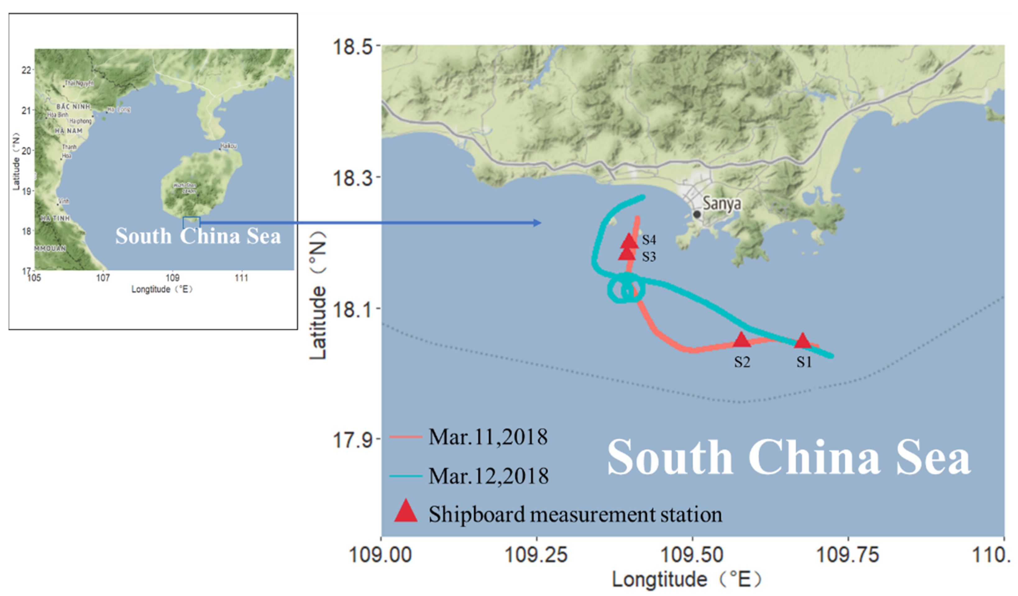
2.1. Study Area
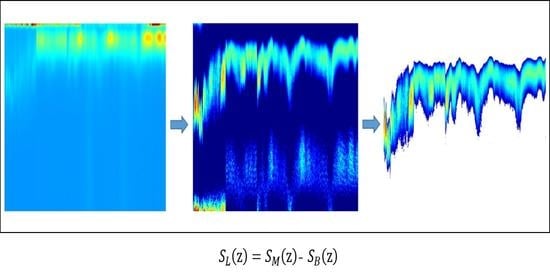
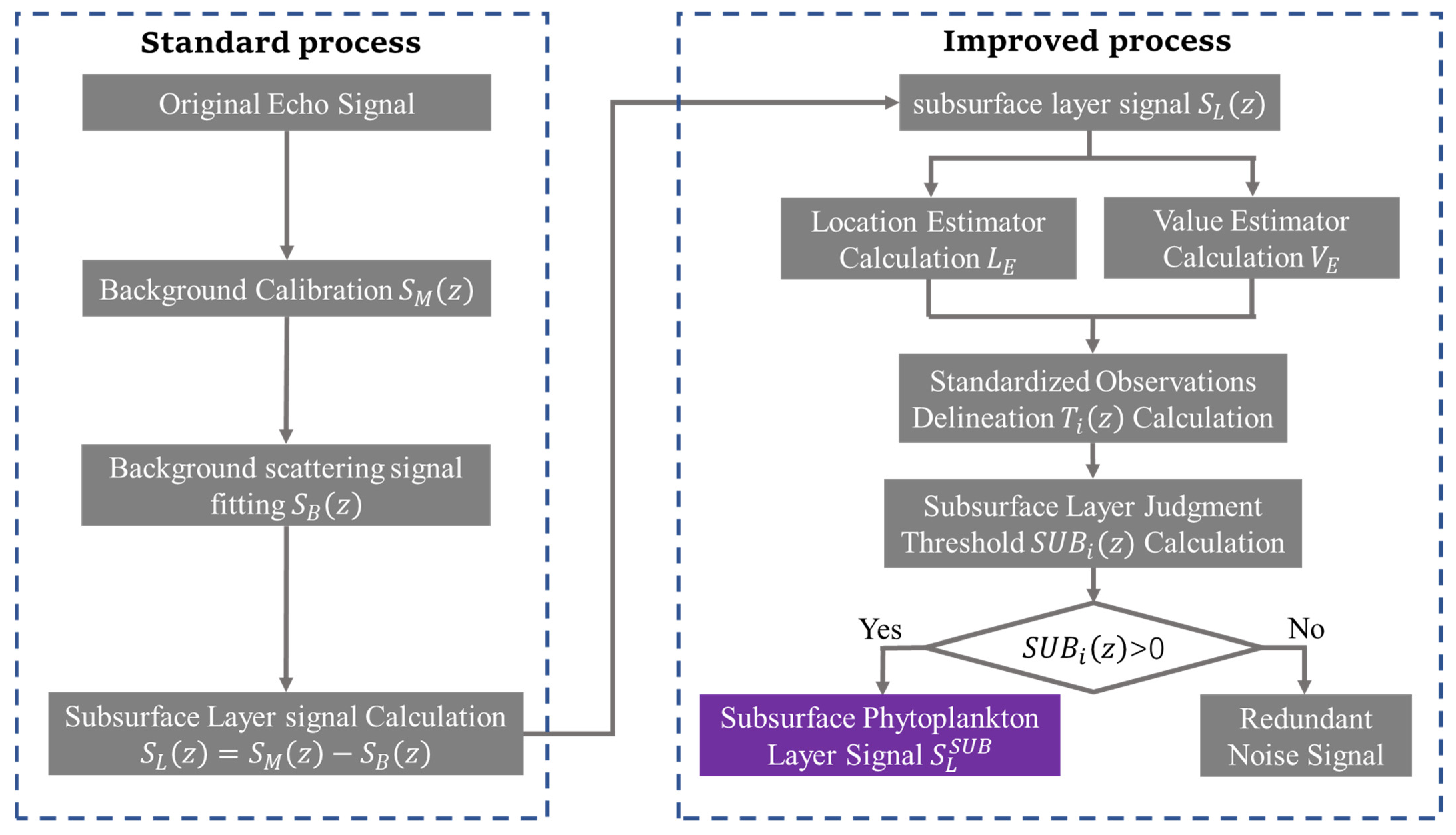
2.2. IASPLDM
3. Result
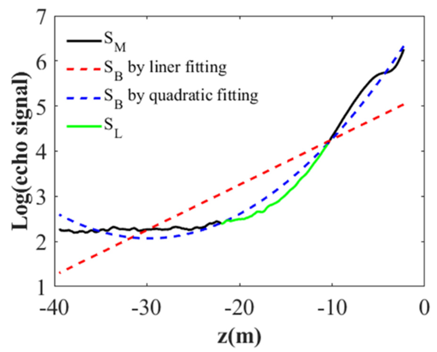
3.1. Example Results for Step-By-Step Process of IASPLDM
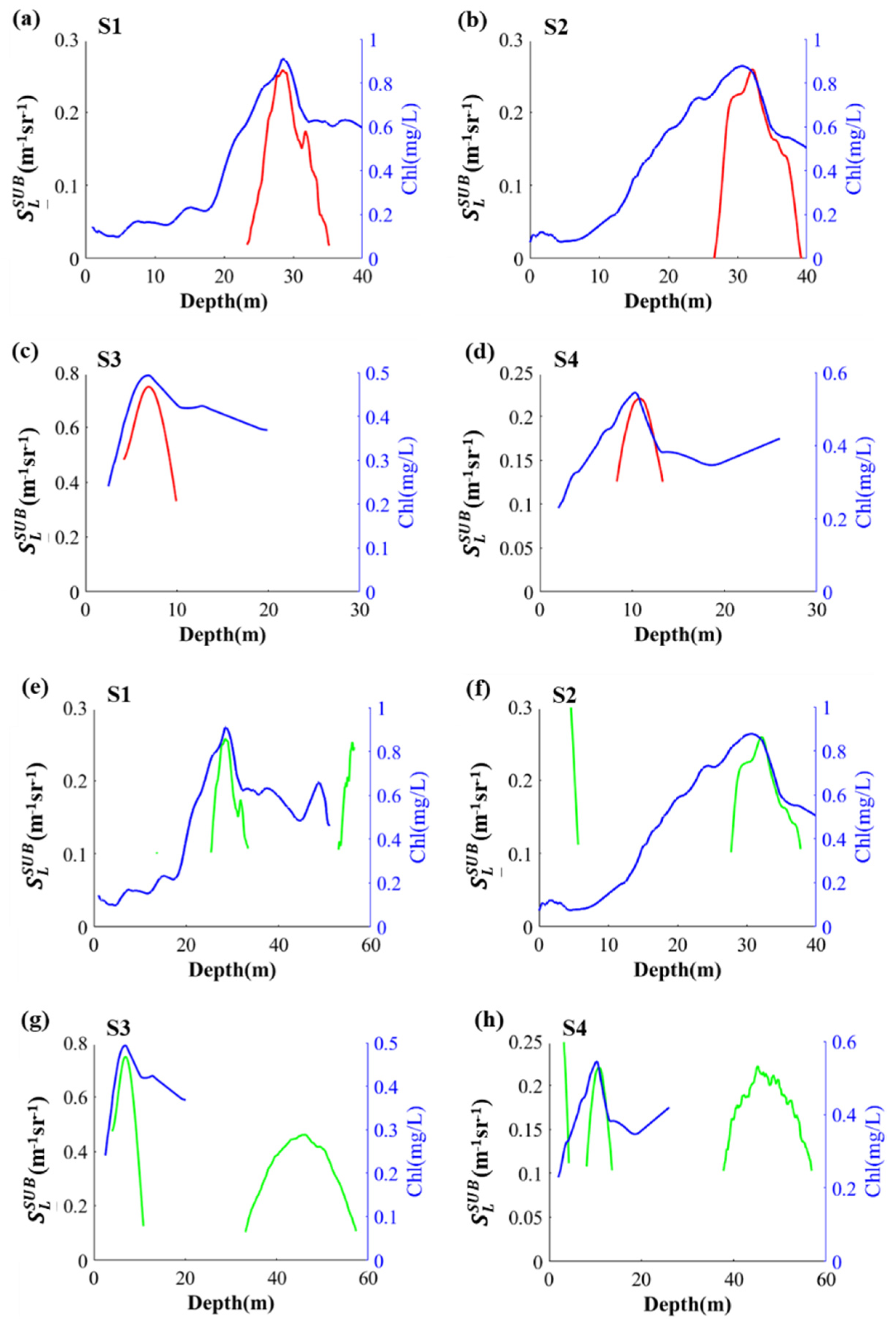
3.2. Retrieval Comparisons between the Standard and the Improved Method
3.3. Algorithm Verification
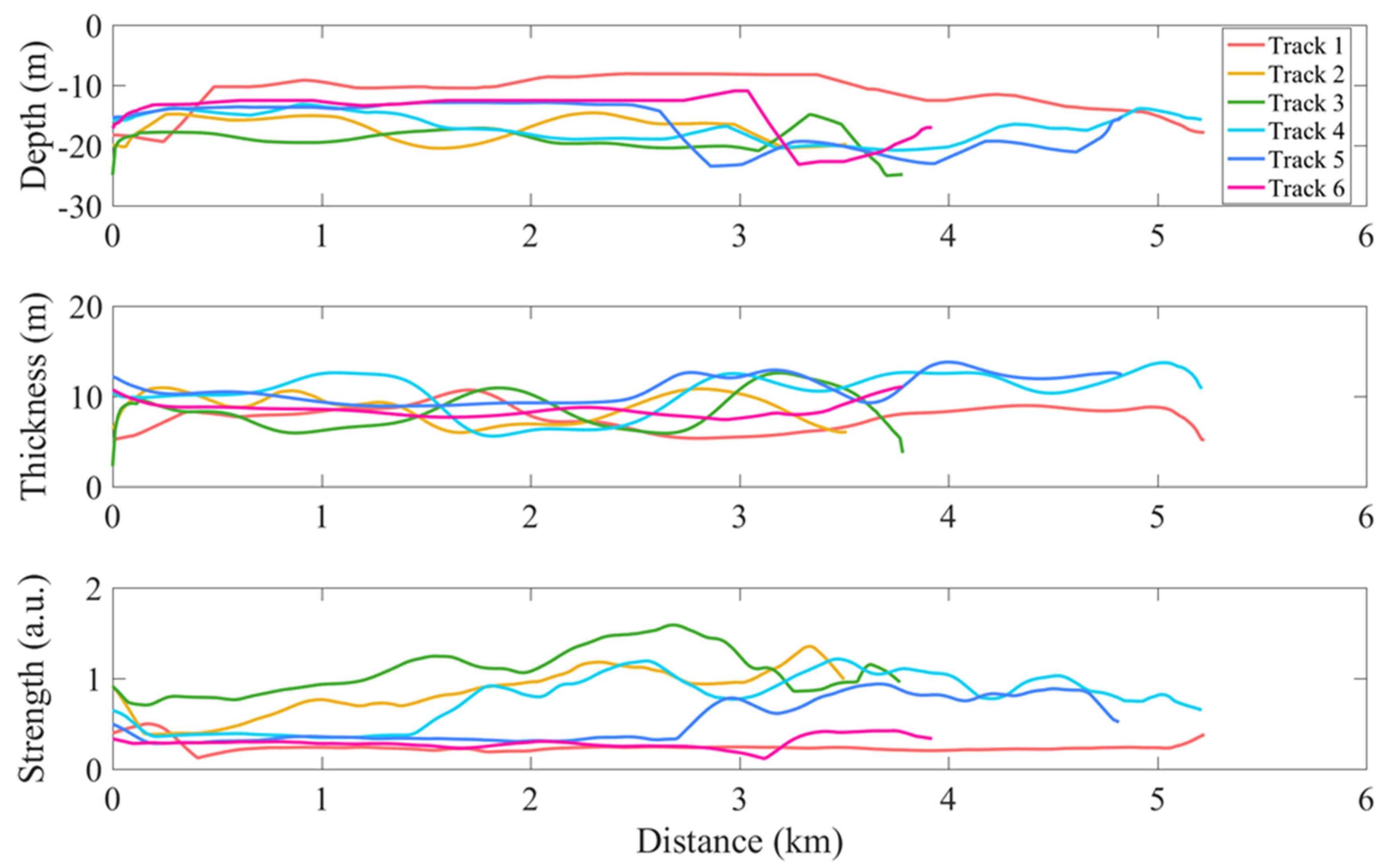
3.4. Application in Lidar Track Data in the Seawater near Wuzhizhou Island
4. Discussion
5. Conclusions
Author Contributions
Funding
Data Availability Statement
Acknowledgments
Conflicts of Interest
References
- Hostetler, C.; Behrenfeld, M.J.; Hu, Y.; Hair, J.W.; Schulien, J.A. Spaceborne Lidar in the Study of Marine Systems. Annu. Rev. Mar. Sci. 2018, 10, 121–147. [Google Scholar] [CrossRef] [Green Version]
- Daniel, G.B.; Marlon, R.L.; Boris, W. Global phytoplankton decline over the past century. Nature 2011, 466, 591–596. [Google Scholar]
- Yue, C.; Zhibin, J.; Lu, S.; Genhai, Z.; Zhifu, W.; Yibo, L.; Yuexin, G. Distribution of net-collected phytoplankton and influence environmental factors in spring and autumn in the adjacent waters near Qinshan Nuclear Power Plant. Mar. Sci. Bull. 2018, 37, 31–39. [Google Scholar]
- Hongzhen, T.; Qinping, L.; Goes, J.I.; Gomes, H.D.R.; Mengmeng, Y. Temporal and spatial changes in chlorophyll a concentrations in the Bohai Sea in the past two decades. Hai Yang Xue Bao 2019, 41, 131–140. [Google Scholar]
- Dekshenieks, M.M.; Donaghay, P.L.; Sullivan, J.M.; Rines, J.E.B.; Osborn, T.R.; Twardowski, M.S. Temporal and spatial occurrence of thin phytoplankton layers in relation to physical processes. Mar. Ecol. Prog. 2001, 223, 61–71. [Google Scholar] [CrossRef]
- Chumside, J.H.; Donaghay, P.L. Thin scattering layers observed by airborne lidar. ICES J. Mar. Sci. 2009, 66, 778–789. [Google Scholar] [CrossRef]
- Sullivan, J.M.; Donaghay, P.L.; Rines, J.J.C.S.R. Coastal thin layer dynamics: Consequences to biology and optics. Cont. Shelf. Res. 2010, 30, 50–65. [Google Scholar] [CrossRef]
- Schulien, J.A.; Penna, A.D.; Gaube, P.; Chase, A.; Behrenfeld, M.J. Shifts in Phytoplankton Community Structure Across an Anticyclonic Eddy Revealed from High Spectral Resolution Lidar Scattering Measurements. Front. Mar. Sci. 2020, 7, 349. [Google Scholar] [CrossRef]
- Kostadinov, T.S.; Siegel, D.A.; Maritorena, S. Global variability of phytoplankton functional types from space: Assessment via the particle size distribution. Biogeosciences 2010, 7, 3239–3257. [Google Scholar] [CrossRef] [Green Version]
- Werdell, P.J.; Roesler, C.S.; Goes, J.I. Discrimination of Phytoplankton Functional Groups Using an Ocean Reflectance Inversion Model. Appl. Opt. 2014, 53, 4833–4849. [Google Scholar] [CrossRef]
- Uitz, J.; Stramski, D.; Reynolds, R.A.; Dubranna, J. Assessing phytoplankton community composition from hyperspectral measurements of phytoplankton absorption coefficient and remote-sensing reflectance in open-ocean environments. Remote Sens. Environ. 2015, 171, 58–74. [Google Scholar] [CrossRef]
- Mouw, C.B.; Hardman-Mountford, N.J.; Alvain, S.; Bracher, A.; Brewin, R.J.W.; Bricaud, A.; Ciotti, A.M.; Devred, E.; Fujiwara, A.; Hirata, T.; et al. A Consumer’s Guide to Satellite Remote Sensing of Multiple Phytoplankton Groups in the Global Ocean. Front. Mar. Sci. 2017, 4, 41. [Google Scholar] [CrossRef] [Green Version]
- Chen, P.; Pan, D. Ocean Optical Profiling in South China Sea Using Airborne LiDAR. Remote Sens. 2019, 11, 1826. [Google Scholar] [CrossRef] [Green Version]
- Peng, C.; Pan, D.; Mao, Z.; Hang, L. A Feasible Calibration Method for Type 1 Open Ocean Water LiDAR Data Based on Bio-Optical Models. Remote Sens. 2019, 11, 172. [Google Scholar]
- Xiao-long, L.; Chaofang, Z. Application and development of Lidar to detect the vertical distribution of marine materials. Infrared Laser Eng. 2020, 49, 24–32. [Google Scholar]
- Chen, P.; Jamet, C.; Mao, Z.; Pan, D. OLE: A Novel Oceanic Lidar Emulator. IEEE Trans. Geosci. Remote Sens. 2020, 99, 1–15. [Google Scholar] [CrossRef]
- Churnside, J.H.; Ostrovsky, L.A. Lidar observation of a strongly nonlinear internal wave train in the Gulf of Alaska. Int. J. Remote Sens. 2005, 26, 167–177. [Google Scholar] [CrossRef]
- Churnside, J.H.; Marchbanks, R.D.; Lee, J.H.; Shaw, J.A.; Weidemann, A.; Donaghay, P.L. Airborne lidar detection and characterization of internal waves in a shallow fjord. J. Appl. Remote Sens. 2012, 6, 063611. [Google Scholar] [CrossRef] [Green Version]
- Chen, P.; Pan, D.; Mao, Z.; Liu, H. Semi-Analytic Monte Carlo Model for Oceanographic Lidar Systems: Lookup Table Method Used for Randomly Choosing Scattering Angles. Appl. Sci. 2019, 9, 48. [Google Scholar] [CrossRef] [Green Version]
- Liu, H.; Chen, P.; Mao, Z.; Pan, D. Iterative retrieval method for ocean attenuation profiles measured by airborne lidar. Appl. Opt. 2020, 59, C42–C51. [Google Scholar] [CrossRef]
- Chen, P.; Pan, D.; Mao, Z.; Liu, H. Semi-analytic Monte Carlo radiative transfer model of laser propagation in inhomogeneous sea water within subsurface plankton layer. Opt. Laser Technol. 2019, 111, 1–5. [Google Scholar] [CrossRef]
- Chen, P.; Jamet, C.; Zhang, Z.; He, Y.; Mao, Z.; Pan, D.; Wang, T.; Liu, D.; Yuan, D. Vertical distribution of subsurface phytoplankton layer in South China Sea using airborne lidar. Remote Sens. Environ. 2021, 263, 112567. [Google Scholar] [CrossRef]
- Chen, P.; Mao, Z.; Zhang, Z.; Liu, H.; Pan, D. Detecting subsurface phytoplankton layer in Qiandao Lake using shipborne lidar. Opt. Express 2020, 28, 558–569. [Google Scholar] [CrossRef]
- Liu, H.; Chen, P.; Mao, Z.; Pan, D.; He, Y. Subsurface plankton layers observed from airborne lidar in Sanya Bay, South China Sea. Opt. Express 2018, 26, 29134–29147. [Google Scholar] [CrossRef]
- Goldin, Y.A.; Vasilev, A.N.; Lisovskiy, A.S.; Chernook, V.I. Results of Barents Sea airborne lidar survey. In Current Research on Remote Sensing, Laser Probing, & Imagery in Natural Waters; International Society for Optics and Photonics: Bellingham, WA, USA, 2007. [Google Scholar]
- Zimmerman, R.C. Estimates of primary production by remote sensing in the Arctic Ocean: Assessment of accuracy with passive and active sensors. Deep Sea Res. Part I Oceanogr. Res. Pap. 2010, 57, 1243–1254. [Google Scholar]
- Churnside, J.H.; Marchbanks, R.D. Subsurface plankton layers in the Arctic Ocean. Geophys. Res. Lett. 2015, 42, 4896–4902. [Google Scholar] [CrossRef]
- Churnside, J.H.; Marchbanks, R.D.; Vagle, S.; Bell, S.W.; Stabeno, P.J. Stratification, plankton layers, and mixing measured by airborne lidar in the Chukchi and Beaufort seas. Deep Sea Res. Part II Top. Stud. Oceanogr. 2020, 177, 4742. [Google Scholar] [CrossRef]
- Behrenfeld, M.J.; Hu, Y.; O’Malley, R.T.; Boss, E.S.; Hostetler, C.A.; Siegel, D.A.; Sarmiento, J.L.; Schulien, J.; Hair, J.W.; Lu, X.; et al. Annual boom–bust cycles of polar phytoplankton biomass revealed by space-based lidar. Nat. Geosci. 2016, 10, 118–122. [Google Scholar] [CrossRef]
- Churnside, J.H.; Tenningen, E.; Wilson, J.J. Comparison of data-processing algorithms for the lidar detection of mackerel in the Norwegian Sea. ICES J. Mar. Sci. 2009, 66, 1023–1028. [Google Scholar] [CrossRef]
- Rousseeuw, P. Robust Estimation and Identifying Outliers. In Handbook of Statistical Methods for Engineers and Scientists; McGraw-Hill: New York, NY, USA, 1998; pp. 16.2–16.4. [Google Scholar]
- Zhong, C.; Yin, F.; Zhang, J.; Zhang, S.; Kitazawa, D. Optimized Algorithm for Processing Outlier of Water Current Data Measured by Acoustic Doppler Velocimeter. J. Mar. Sci. Eng. 2020, 8, 655. [Google Scholar] [CrossRef]


| Source | SS | df | MS | F | p Value |
|---|---|---|---|---|---|
| Groups | 0.485 | 1 | 0.485 | 0 | 0.9571 |
| Error | 925.548 | 6 | 154.258 | ||
| Total | 926.033 | 7 |
| Source | SS | df | MS | F | p Value |
|---|---|---|---|---|---|
| Groups | 6.2965 | 1 | 6.29651 | 1.05 | 0.3456 |
| Error | 36.0771 | 6 | 6.01286 | ||
| Total | 42.3737 | 7 |
Publisher’s Note: MDPI stays neutral with regard to jurisdictional claims in published maps and institutional affiliations. |
© 2021 by the authors. Licensee MDPI, Basel, Switzerland. This article is an open access article distributed under the terms and conditions of the Creative Commons Attribution (CC BY) license (https://creativecommons.org/licenses/by/4.0/).
Share and Cite
Zhong, C.; Chen, P.; Pan, D. An Improved Adaptive Subsurface Phytoplankton Layer Detection Method for Ocean Lidar Data. Remote Sens. 2021, 13, 3875. https://doi.org/10.3390/rs13193875
Zhong C, Chen P, Pan D. An Improved Adaptive Subsurface Phytoplankton Layer Detection Method for Ocean Lidar Data. Remote Sensing. 2021; 13(19):3875. https://doi.org/10.3390/rs13193875
Chicago/Turabian StyleZhong, Chunyi, Peng Chen, and Delu Pan. 2021. "An Improved Adaptive Subsurface Phytoplankton Layer Detection Method for Ocean Lidar Data" Remote Sensing 13, no. 19: 3875. https://doi.org/10.3390/rs13193875