Article

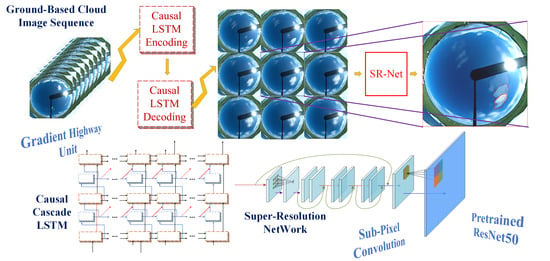
A Method of Ground-Based Cloud Motion Predict: CCLSTM + SR-Net

1
School of Electrical and Information Engineering, Tianjin University, Tianjin 300072, China
2
School of Information Science and Engineering, Shandong Normal University, Jinan 250014, China
*
Author to whom correspondence should be addressed.
Remote Sens. 2021, 13(19), 3876; https://doi.org/10.3390/rs13193876
Submission received: 30 July 2021 / Revised: 22 September 2021 / Accepted: 24 September 2021 / Published: 28 September 2021

Abstract

:
Ground-based cloud images can provide information on weather and cloud conditions, which play an important role in cloud cover monitoring and photovoltaic power generation forecasting. However, the cloud motion prediction of ground-based cloud images still lacks advanced and complete methods, and traditional technologies based on image processing and motion vector calculation are difficult to predict cloud morphological changes. In this paper, we propose a cloud motion prediction method based on Cascade Causal Long Short-Term Memory (CCLSTM) and Super-Resolution Network (SR-Net). Firstly, CCLSTM is used to estimate the shape and speed of cloud motion. Secondly, the Super-Resolution Network is built based on perceptual losses to reconstruct the result of CCLSTM and, finally, make it clearer. We tested our method on Atmospheric Radiation Measurement (ARM) Climate Research Facility TSI (total sky imager) images. The experiments showed that the method is able to predict the sky cloud changes in the next few steps.

Graphical Abstract

1. Introduction

Cloud observations are mainly divided into space-based satellites, air-based radiosondes and ground-based remote sensing observations. Air-based radiosonde observation has advantages in detecting the vertical structure of the cloud, but it is difficult to meet the requirements of actual cloud detection due to its high cost and low detection frequency [1]. Space-based satellite observations cannot provide enough temporal and spatial resolution for local and short-term cloud analyses in specific areas [2]. The deficiency of air-based radiosonde and space-based satellite remote sensing observation leads to the popularization of ground-based remote sensing observations, especially cloud image observations, which can provide strong support for satellite and radiosonde observation. These images are low-cost and high-resolution, which can provide accurate local sky cloud information [1].
Ground-based cloud images have a wide range of applications in many fields, such as weather condition monitoring [3], cloud cover monitoring [4], photovoltaic power generation system [5], remote sensing and atmospheric research, air pollution and prevention [6], etc. Compared with satellite cloud images, ground-based cloud images have a smaller observation range and coverage, which can only show sky cloud conditions within a radius of tens of kilometers of the observation site. However, it includes many cloud details, which can better reflect the cloud thickness, height, volume and category [7].
Forecast data for the next few moments is often hoped for timely observation research, so that some targeted operations can be carried out. For example, for photovoltaic power generation systems, the photovoltaic output slope events caused by the motion of clouds and the occlusion of the sun require manual intervention by photovoltaic power stations to compensate. Predicting the occurrence of such events is conducive to improving the operation and management efficiency of photovoltaic power stations [8]. Therefore, research on cloud motion and short-term cloud tracking emerged. At present, many research methods for predicting cloud motion have been proposed. Dissawa et al. [8] proposed a short-term cloud tracking method based on cross-correlation and the Lukas-Kanade optical flow algorithm. El Jaouhari et al. [9] proposed a ground-based cloud image omnidirectional optical flow tracking method. Dissawa et al. [10] proposed cloud motion estimation based on cross-correlation to predict short-term solar irradiance. In Jamaly’s research [11], quality control was added to the cross-correlation method and cross-spectral analysis, and the cloud motion was estimated by analyzing the spatiotemporal correlation of the irradiance data. The common point of these methods is that they cannot obtain the future cloud state visually, and the future cloud state is often described by other variables, such as the cloud motion vector.
Neural network and deep learning are also used in the research of ground-based cloud images, but in most cases, they are used for cloud recognition and cloud classification [12,13,14,15,16]. In fact, the prediction of cloud motion in a ground-based cloud image can also be directly obtained from the images generated by the neural network. Since the location of the sky imager that collected the ground-based cloud images is fixed for a long time, the other elements of the obtained cloud images remain basically unchanged, except the cloud motion. Therefore, a deep learning generation model can be established, taking real cloud images at several historical moments as the input to generate simulated cloud images at several future moments. In this way, cloud motion prediction is transformed into image sequence prediction.
In recent years, a variety of algorithms have been proposed for image sequence prediction. For example, ConvLSTM [17], PredRNN and its enhanced version [18,19], Cubic LSTM [20], GAN + LSTM [21], DRNet [22], etc. Most of these models have been tested on the Moving MNIST and KTH datasets and have achieved inspiring results.
However, compared with the Moving MNIST and KTH datasets, cloud motion is more complex and changeable, whose shape, contour and movement patterns are more difficult to predict. In addition, ground-based cloud images have a higher resolution than images such as handwritten numbers, which will cause an unbearable consumption of training resources. Therefore, it is difficult for a conventional prediction model to complete the cloud image sequence prediction task separately. In the research of Su et al. [23], a convolutional network Multi-GRU-RCN was used to predict satellite cloud images. However, their research only completed the prediction of the next frame of the grayscale image sequence.
Video-related image sequence predictions often have shorter time intervals between frames [24,25], and the sampling frequency is tens of times per second. The whole sky imager usually would not set such a high sampling frequency, which would result in excessive storage requirements. Moreover, the predictions for the subsequent dozens of moments still stay within the same second, which is too short for other subsequent studies. The sampling interval of ground-based cloud images is usually set to 30 s [26]. This leads to a large difference between each frame of the cloud image sequence, which brings greater difficulties to the prediction.
In this paper, we propose a cloud motion prediction method based on a two-stage framework shown in Figure 1. We perform a low-resolution cloud motion prediction in the first stage and retrieve high-frequency components in the second stage. In the first stage, Cascade Causal Long Short-Term Memory (CCLSTM) is used as the basic prediction model. It is responsible for the preliminary cloud motion prediction and contour change prediction at a low resolution. A custom image generation network and pretrained ResNet50 are used as the super-resolution model in the second stage. They are responsible for reconstructing the prediction results of low resolution into high resolution and improving the image quality.
Due to the unpredictability of cloud motion and the pre-downsampling (see Section 2.2), the result obtained by the CCLSTM can only give a rough contour boundary of the cloud, which is not conducive to the subsequent feature extraction and prediction work. Therefore, the super-resolution model is used for fine reconstruction of the prediction results, in which a loss function is used to supplement the high-frequency components. The details are provided in Section 3. Compared with the traditional methods based on digital image processing and cloud motion vector estimation [8,9,10,11], the advantages of this method are summarized as follows:
  • Traditional methods mostly use single-channel grayscale images or binary images after cloud recognition. The prediction results of this method can obtain RGB three-channel color images, which can be extracted with features such as the red–blue ratio;
  • Traditional methods can only predict the direction of cloud motion. This method can predict the cloud contour changes while predicting the cloud motion trajectory;
  • Traditional methods have to perform distortion correction, shading belt filtering and other preprocessing. In contrast, this method directly obtains the prediction results without any preprocessing. This is helpful for extracting more features, such as the reflection intensity of the shading belt to sunlight (the shading belt is not pure black reflected in the figure) and so on;
  • This method can continuously give cloud motion prediction results at multiple moments, and they all have high reliability.
The paper is organized as follows: Section 2 introduces the necessary preparations made before the whole model training. Section 3 introduces the construction of the CCLSTM and its temporary results. Section 4 introduces the super-resolution model and its effects. Section 5, Section 6 and Section 7 are the results, discussion and conclusion, respectively.

2. Training Preparation

2.1. Training Image Dataset

The training data was collected by TSI-880 equipment provided by the Atmospheric Radiation Measurement (ARM) Climate Research Facility. The images were taken at 39.0916°N, 28.0257°W: Eastern North Atlantic (ENA) Graciosa Island, Azores, Portugal.
From February 17, 2016 to April 29, 2016, a total of 37,540 ground-based cloud images were selected as a dataset to cover as much as possible the sunny, cloudy, overcast, etc. images in various time periods from 6 a.m. to 18:00 p.m. at the local time. The number of images used by each model is shown in Table 1.

2.2. Image Preprocessing

Before training, it is necessary to preprocess the original images, as shown in Figure 2.
First, clip the unnecessary information around, and only keep the smallest circumscribed rectangle containing the spherical mirror. Secondly, downsample the clipped images. The size of the image was clipped from 640 × 480 to 440 × 440. Due to the complexity of image sequence regression and the need to take up large computing resources, we used pre-downsampling to reduce the scale of the model parameters and the number of calculations to release a certain degree of GPU memory space. This is conducive to set more reasonable training parameters, such as the batch size. We tried to downsample the cloud images to 64 × 64, 96 × 96 and 128 × 128 by bicubic linear interpolation and, finally, chose a moderate scheme of 96 × 96, which can keep more original image information as much as possible on the premise of reducing the training cost.

2.3. Experimental Equipment

The model was trained with Intel i7 9700 CPU, RTX 2080 super 8G GPU and 32GB RAM. The running environment was Windows 10, Python 3.7.7, tensorflow 1.14.0 (A symbolic mathematics system based on data flow programming), CUDA 10.2 (A computing platform launched by NVIDIA), cudnn 7.6.5 (A GPU acceleration library for deep neural networks) and keras 2.3.1 (An open-source neural network library).

3. Prediction Model

3.1. Cascade Causal LSTM

The key of the image sequence prediction is the combination of temporal information and spatial information. LSTM can transmit temporal information but cannot transmit spatial information. The Convolutional Neural Network (CNN) can transmit spatial information effectively, but it is difficult to transmit temporal information. The proposal of ConvLSTM [17] solved the problem of the combined transmission of temporal and spatial information to a certain extent. However, its short-term dynamic modeling ability is insufficient to get better prediction results for complex problems. Therefore, it is necessary to strengthen the model in terms of short-term dynamic modeling and spatial correlation.
The basic structure of CCLSTM is derived from PredRNN++ [19]. We named it by free translation. The input information of the CCLSTM is a historical cloud image sequence, and the sequence length can be determined according to the situation (here, it is 10). It will output a sequence of future cloud images with a preset length (here, also 10). The causal LSTM is a cascade structure; it is composed of two structures that process temporal and spatial information in a series and merge them before transmit to the next cell. Its basic cell includes a long-term temporal state C t k , a spatial state M t k and a current hidden state H t k . X t is the input information. The subscript t is the time stamp, and the superscript k is the corresponding number of layers in the network. The unit temporal state C t k is jointly controlled by the forget gate f t , input gate i t and modulation gate g t . The cell is shown in Figure 3. A concentric circle represents the splicing of the multi-dimensional array on the last dimension, σ is the sigmoid function and the × and + in the circle represent the multiplication and addition of the corresponding elements of the array.
We use a double-layer 3 × 3 convolution filter to replace the single-layer 5 × 5 convolution filter in PredRNN++. The one point in the red circle in Figure 3 is our double-layer convolution filter, which contains the convolution layer, batch normalization layer and Rectified Linear Unit (ReLU) layer, and its structure is shown in Figure 4. The first convolution layer of the double-layer convolution filter contains nonlinear ReLU activation, and the second layer does not, because the nonlinear functions “tanh” and “sigmoid” in the LSTM will be connected later. The benefits of this are:
  • Reduce the parameters of the model with the same receptive field;
  • Increase the network depth within a unit and enhance the unit’s fitting ability.
The equations of the Causal LSTM can be presented as follows:
g t = tanh d o u b l e c o n v [ X t , H t 1 k , C t 1 k ]
i t = σ d o u b l e c o n v [ X t , H t 1 k , C t 1 k ]
f t = σ d o u b l e c o n v [ X t , H t 1 k , C t 1 k ]
C t k = f t × C t 1 k + i t × g t
g t = tanh d o u b l e c o n v [ X t , M t k 1 , C t k ]
i t = σ d o u b l e c o n v [ X t , M t k 1 , C t k ]
f t = σ d o u b l e c o n v [ X t , M t k 1 , C t k ]
M t k = f t × tanh ( d o u b l e c o n v [ M t k 1 ] ) + i t × g t
o t = tanh ( d o u b l e c o n v [ X t , C t k , M t k , H t 1 k ] )
H t k = o t × tanh ( d o u b l e c o n v [ C t k , M t k ] )
In the above equations, × means the multiplication of the corresponding elements in the multidimensional array, and in A B means that function A acts on array B .
While deepening the network, the gradient communication channels also need to be strengthened. In order to provide a gradient path for the abstract expression of vertical spatial information, we used a spaced LSTM vertical layer and inserted a gradient highway unit (GHU) layer between each layer of causal LSTM cells. At the same time, in order to make the horizontal temporal sequence unit L t k receive the gradient of the previous unit L t 1 k 1 in the previous layer timelier, we added a jumper between the input and output of the lower layer GHU. In this way, the useful part of the gradient information can be passed into L t k through only one GHU instead of two. The combination of jumpers is array splicing and convolution. CCLSTM is an interval structure with a total of 5 layers, and the number of convolution channels in each layer is set to 64, 64, 32, 32 and 32, as shown in Figure 5. The dotted line indicates that it is connected to the next-order unit not shown.
The GHU is shown in Figure 6. One point in the circle represents the convolution and batch normalization. Double-layer convolution filters are not used in the GHU, because increasing the unit depth is contrary to the original intention of the gradient highway. σ is the sigmoid function, and the × and + in the circle represent the multiplication and addition of the elements at the corresponding positions in the array, respectively.
The equations of the GHU can be presented as follows:
S t = σ ( c o n v [ Z t 1 ] + c o n v [ H t ] )
P t = tanh ( c o n v [ Z t 1 ] + c o n v [ H t ] )
Z t = P t × S t + Z t 1 × ( 1 S t )
Equations of the CCLSTM can be presented as follows:
Z t k = G H U ( H t k 1 , Z t 1 k )
when k is equal to 1:
H t 1 , C t 1 , M t 1 = C a u s a l L S T M 1 ( X t , H t 1 1 , C t 1 1 , M t 1 L )
when k is not equal to 1:
H t k , C t k , M t k = C a u s a l L S T M k ( c o n v [ Z t 1 , Z t ] , H t 1 k , C t 1 k , M t k 1 )
In the above equations, while a variable does not exist, it is regarded as 0, such as X 11 . L is the total number of vertical layers. In Equation (15), L is taken as 5.

3.2. Prediction Results of CCLSTM

Figure 7 shows the prediction results of the CCLSTM under various conditions, such as sunny, partly cloudy, cloudy and overcast. The length of the input sequence and output sequence are both set to 10. It means that, after inputting historical cloud images with a total length of 5 min, 10 predicted cloud images with an interval of 30 s in the next 5 min will be obtained. The batch size and learning rate are set to 8 and 0.002, respectively.
Figure 8 shows the changes in the validation set evaluation of CCLSTM and the original PredRNN++ during the training process. The calculation method of the Mean Squared Error (MSE) is shown in Equation (17), where n is the total number of pictures in the verification set, m is the number of pixels in each image and φ represents the value of pixels normalized to “0 to 1”.
M S E = 1 n n i = 1 m ( φ i φ ^ i ) 2
Except for the structural adjustment described in Section 3.1, the two models are consistent in other hyperparameters and dataset distributions. It can be seen that both the two schemes reach the optimal point at about 50,000 training iterations. Compared with the original version, CCLSTM has a certain improvement in the decline speed in the early stage and the optimal results in the later stage. In fact, when the training iterations reach 20,000, the MSE value of CCLSTM on the validation set is already lower than the global minimum value of the original scheme.

3.3. Ablation Study

We conducted many training attempts for different structures of the model, and the model with the best overall effect is described in Section 3.1. The remaining models are:
  • The original PredRNN++;
  • The original PredRNN++ with a double number of filters in the convolution layers;
  • CCLSTM with no ReLU activation function between the double-layer convolution filter compared with the final version;
  • CCLSTM, which does not contain a double-layer convolution filter and jumpers compared with the final version;
  • A 7-layer structure with 4 layers of Causal LSTM cells interleaved with 3 layers of GHUs;
  • The original PredRNN++ with the vertical depth increased by one layer.
Taking the Peak Signal-to-Noise Ratio (PSNR [27]) and Structural Similarity (SSIM [28]) commonly used in image comparison and evaluation metrics, the test results of these models in the test set of 480 various weather conditions are shown in Table 2.
It can be seen that, for PSNR, our final scheme (5 layers) obtained the best results at sequences 1, 3, 4, 6 and 7. The sequences 2 and 5 were slightly weaker than the double-layer convolution fliter without ReLU, but the gap was not large. This did not rule out accidental phenomena caused by factors such as model initialization. The prediction results of images 8, 9 and 10 were weaker than the 7-layer interval scheme. This shows that vertically deepening the network layer and setting the GHU layer in time could help to better carry out gradient propagation. Of course, it would also increase the consumption of the training resources accordingly. For SSIM, our scheme had the best performance in the first 9 images, only slightly weaker than the 7-layer interval structure in the last image. It fully proved the effectiveness of our gradient enhancement scheme.

4. Super-Resolution Reconstruction of Predicted Images

In order to reduce the resource requirements for training and the number of model parameters, the original images were downsampled to 96 × 96 pixels. However, the prediction results utilizing small size images cannot meet the subsequent research needs. Therefore, we established a super-resolution reconstruction model to restore the predicted images to a certain extent.
Although CCLSTM can predict the subsequent displacement and contour of the cloud to a certain extent, it cannot give a result with a clear cloud boundary (as shown in Section 3.2). Since the ground-based cloud image is a two-dimensional image displayed from the ground perspective and does not contain three-dimensional information, it is impossible to obtain all the data about cloud changes from the image. Therefore, the blur contained in the output images is actually expected. In addition, the prediction model used L2 loss to get a better PSNR, which would cause the result to become smooth and increase the fuzziness of the output images. Therefore, an enhanced model is needed to further process the prediction results, supplement the detailed information lost due to downsampling, clarify the cloud boundary and facilitate subsequent researches, such as feature extraction for direct normal irradiance prediction and photovoltaic power regression [29].
In recent years, some progress has been made in the methods of making various kinds of fuzzy images clearer. For example, a generative adversarial network is used to approximate the super-resolution result of the image [30]. Balakrishnan et al. [31] mentioned that, through convolution and deconvolution operations, the fuzzy situation caused by camera shaking can be recovered from the perspective of probability. In the research of Ye et al. [32], a CNN-based architecture is reported to detect unsharp masking (USM). Lai et al. [33] proposed a fast and accurate super-resolution based on a deep Laplacian pyramid network, etc.
Considering the limited computing resources, the super-resolution model in our research does not have to be too complicated. A model that can complete the established task is sufficient.

4.1. Super-Resolution Network

For image clarification processing, an image generation model is first required. The generation model has a total of 10 layers of convolution, of which the first and second layers use dilated convolution [34]. This is made to expand the receptive field in the convolution layer closest to the low-dimensional features of the original images. The size of the convolution kernel is 3 × 3, and the number of convolution filters is 64. The 3rd–8th layers are conventional convolution, in which the size of the convolution kernel is 3 × 3, and the number of filters is 64. The ninth layer utilizes sub-pixel convolution [35] to expand the 96 × 96 feature map to 192 × 192, in which the number of convolution filters is 128, and it will become 32 channels after convolution. The last layer is also a sub-pixel convolution, in which the number of filters is 12. After convolution, it will become 3 channels, and the image size will become 384 × 384. Since image generation is a regression problem, no activation is set in the last layer. In addition, all the previous layers use LeakyReLU as a nonlinear activation function. Compared with ReLU, it can solve the problem of CNN node death in the transformation process. The slope of LeakyReLU on the negative semi-axis is set to 0.03. The structure of the super-resolution generation model is shown in Figure 9.

4.2. Perceptual Losses

We tried to use the super-resolution generation network and pixel-level MSE for resolution restoration, but the results were unsatisfactory, because it would make the generated images over-smooth. It was proved that using the MSE or Mean Absolute Error (MAE) as the loss function cannot fundamentally solve the problem of the lack of high-frequency components of the image. Perceptual loss [36] has been proven to have a good effect on this issue. Perceptual loss utilizes the feature extraction ability of the pretrained model to adjust the training direction and retain more detailed features, which realizes error back propagation by calculating the difference of the feature map between the generated image and the real image. The deep convolutional network VGG [37] is commonly used as the pretrained model while training image transfer networks deal with perceptual loss [36,38,39,40,41]. However, from the training results of the ImageNet dataset, the feature extraction ability of ResNet is stronger than VGG. Considering the complexity of the model and the number of parameters, we chose ResNet50, which is smaller among the various ResNets, as shown in Figure 10.
The inputs in Figure 10 are the outputs of CCLSTM, which have low resolution. After the Super-resolution Network, they are passed along with the Ground Truths to the pretrained ResNet50. Then, some feature map errors are added into the model loss to help train the Super-resolution Network.
For the selection of the perceptual loss feature layer, we used the superimposed layer after the last layer of residual blocks at each scale of the feature map. This was to make the features of each scale as high-dimensional as possible. Since L2 loss is more susceptible to differences in the sample distribution, we used the 1-norm as the error distance evaluation standard for each perceptual layer. Suppose that the layer name of the selected feature map block is i , φ represents the elements in the feature map block whose Channels, Height and Width are C , H and W respectively. Then, the perceptual losses can be expressed as:
P L o s s i ( y ^ , y ) = 1 C × H × W b l o c k i φ c , h , w p r e d φ c , h , w t r u e
The total loss can be expressed as:
L o s s ( y ^ , y ) = i m g y t r u e y p r e d 2 2 + i r i × P L o s s i ( y ^ , y )
where r i is the weight of each perceptual layer.
We set the learning rate to manually drop to make the model training converge. The rate of decrease is half of the previous one every 10 epochs.
The error of the output sequence of the prediction model increases gradually from t + 1 to t + 10. For super-resolution reconstruction, there is no correspondence between the input low-resolution image and its ground truth, and the error increases with time. Furthermore, the super-resolution reconstruction model has no inferential ability (or very weak), and artificially adding some inferential concepts would disturb the fitting direction of the model. Therefore, we take all the outputs of the optimal prediction model obtained from the validation set as the training set of the super-resolution reconstruction model. The prediction outputs obtained in this way have correct cloud contours and blurring caused by the pixel-level L2 loss, which meets the requirements.

4.3. Ablation Study of Loss Function

The training data is the 3800 prediction model results containing various cloud conditions and their corresponding real cloud images selected from the super-resolution reconstruction model training set mentioned in Section 4.2. The input size is 96 × 96, and the output is 384 × 384. The ground truths are also rescaled to 384 × 384.
We have made several attempts on the super-resolution model. The tests are as follows:
  • Use the pixel-level MSE as the loss, no dilated convolution and no perceptual loss;
  • Use the L2 perceptual loss, no dilated convolution and all r are taken as 0.05;
  • Use the L1 perceptual loss; no dilated convolution and the values of r 2 , r 3 , r 4 and r 5 are 0.08, 0.04, 0.02 and 0.01. r 1 = 0 ;
  • Use the L1 perceptual loss; no dilated convolution and the values of r 1 , r 2 , r 3 , r 4 and r 5 are 0.04, 0.02, 0.01, 0.01 and 0.05;
  • Use the L1 perceptual loss; no dilated convolution and the values of r 1 , r 2 , r 3 , r 4 and r 5 are 0.002, 0.005, 0.01, 0.02 and 0.04;
  • Use the pixel-level MAE as the loss, with dilated convolution and no perceptual loss;
  • Use the L1 perceptual loss, with dilated convolution and the values of r 1 , r 2 , r 3 , r 4 and r 5 are 0.04, 0.02, 0.01, 0.01 and 0.005.
The results of these tests are shown in order in Figure 11.
It can be seen from the comparison of Figure 11:
  • Comparing (a) with (f), for the carefully selected dataset, the difference between the MSE loss and the MAE loss is not big, and the addition of the dilated convolution makes the result slightly improved;
  • Compare (a)/(f) with other results with added perceptual losses; a pure pixel-level loss will cause the result to be too smooth;
  • Comparing (d) with (g), using dilated convolution to increase the receptive field helps to improve the image quality in some subtleties;
  • Compared with (d) and (e), the increasing and decreasing of the perceptual layers’ weights will bring different degrees of the grid effect. The greater the weight used by the deeper layers in the perceptual model (ResNet50 here), the more serious the grid effect. The severity of the grid effect in the figure is (e) > (b) > (c) > (d) > (g), which is consistent with the selection of r in each plan.
The final choice of r is: r 1 = 0.04, r 2 = 0.02, r 3 = 0.01, r 4 = 0.01 and r 5 = 0.005. It was based on a comprehensive assessment of perception and experience. It should be noted that, for other different datasets or input and output images of different sizes, the above selection of r may not be optimal.

4.4. Super-Resolution Results

Figure 12 is a schematic diagram of the results of the super-resolution model. In order to facilitate the arrangement, images of the different sizes were linearly scaled.
It can be seen from the figure that the original prediction results can restore detailed information to a certain extent after being enhanced by the super-resolution model. At the same time, compared to before the super-resolution, the clouds in the subsequent images are more solid, the edges are clearer and the surrounding scenes such as the shading belt can also be better restored. This is beneficial to other follow-up studies, such as cloud cover monitoring and calculation of the influence of cloud location on solar scattering radiation, etc. It also proves that the final output of the model cannot be affected by the surrounding scenery (no matter what the scenery is); it has a certain degree of robustness.

5. Results

The final results are obtained after super-resolution reconstruction of all the prediction results in Section 3. The time step in the sequence is 30 s. Figure 13 shows the predictable situations and one kind of unpredictable situation of cloud motion.
As shown in Figure 13, t is the current moment, and the green dashed circle indicates that the prediction results are basically correct in response to the real cloud motion. On the contrary, the red dashed circle shows that the cloud motion was not successfully predicted. The PSNR and SSIM of every image in the sequence are shown in Table 3.

6. Discussion

In Figure 13, the cloud moving through the shading belt is difficult to be well-predicted (as shown at t + 5 and thereafter). This is because the shading belt has caused great interference to the actual expression of cloud motion, which is equivalent to a forced gradient disappearance. Cloud formation and extinction occurs frequently during cloud movement, which is particularly serious for small, thin clouds. Therefore, the model cannot determine the state of the clouds when they pass through the shading belt. Experiments show that the model tends to determine the cloud has disappeared.
In addition, under certain circumstances, the input cloud images with similar states may have different fitting targets, resulting in uncertainty of the prediction results. This situation is one of the difficulties in cloud motion prediction and will have a negative impact on the prediction accuracy.
Besides, the wind speed levels can also affect the prediction accuracy. The higher the wind speed, the smaller the number of predicted sequence images that can guarantee a certain accuracy.
In short, in the case of a low wind speed, our model can give relatively correct motion trajectories and contour changes for most clouds that are not affected by factors such as the shading belt.

7. Conclusions

In this paper, we proposed a cloud motion prediction model based on deep learning. To solve the problem of excessive consumption of training resources, we proposed a solution by down-sampling prediction and super-resolution reconstruction. We optimized the model structure of the prediction part and added the loss functions of the reconstruction part.
Compared with the methods of calculating cloud motion vector on binary image, we realized the color cloud image extrapolation without ground scenes removal and distortion correction, obtained continuous sequence images and got relatively accurate results.
Although we improved the over-smoothing problem caused by the pixel-level MSE loss during super-resolution reconstruction, aiming to obtain more high-frequency information, there is still a gap between the final reconstructed result and the real image. Further research is needed to compensate for the lack of image high-frequency components. We also tried to use Generative Adversarial Networks (GAN) to compensate for the high-frequency components of the prediction results, but the current results achieved are not satisfactory. Meanwhile, the GAN methods also bring up some disputes, such as whether the high-frequency information generated by GAN is credible and whether it is beneficial to other subsequent research on predicted cloud images, etc.
In brief, it is still a very difficult task to accurately predict the motion of sky clouds relying on ground-based cloud images. To achieve more accurate predictions, more comprehensive information is needed, such as a high-altitude real-time wind field, upper air temperature variation data and 3D fine modeling of sky clouds. In future research, we will try to introduce new atmospheric physical quantities and add new model structures to get better results.

Author Contributions

Conceptualization, Z.L. and Z.W.; methodology, Z.L.; investigation, Z.L. and Z.W.; software, Z.W.; validation, Z.L., Z.W. and X.L.; formal analysis, Z.W.; data curation, X.L.; writing—original draft preparation, Z.W.; writing—review and editing, Z.L. and J.Z.; project administration, J.Z. and funding acquisition, Z.L. All authors have read and agreed to the published version of the manuscript.

Funding

This research was funded by National Natural Science Foundation of China. Registered number of project approval: 51677123.

Institutional Review Board Statement

Not applicable.

Informed Consent Statement

Not applicable.

Data Availability Statement

For this study, we used an open-source and governmental dataset from the address: Ground-based cloud images from Atmospheric Radiation Measurement (ARM) Climate Research Facility (https://www.arm.gov, accessed on 15 May 2016).

Acknowledgments

The experiment in Section 3 referred to the source code provided by the author of PredRNN++ [19].

Conflicts of Interest

The authors declare no conflict of interest.

References

  1. Wang, Y.; Wang, C.; Shi, C.; Xiao, B. A Selection Criterion for the Optimal Resolution of Ground-Based Remote Sensing Cloud Images for Cloud Classification. IEEE Trans. Geosci. Remote Sens. 2019, 57, 1358–1367. [Google Scholar] [CrossRef]
  2. Dev, S.; Wen, B.; Lee, Y.H.; Winkler, S. Ground-based image analysis: A tutorial on machine-learning techniques and applications. IEEE Geosci. Remote Sens. Mag. 2016, 4, 79–93. [Google Scholar] [CrossRef]
  3. Leveque, L.; Dev, S.; Hossari, M.; Lee, Y.H.; Winkler, S. Subjective Quality Assessment of Ground-based Camera Images. In Proceedings of the 2019 Photonics & Electromagnetics Research Symposium-Fall (PIERS-FALL), Xiamen, China, 17–20 December 2019; IEEE: Piscataway, NJ, USA, 2019; pp. 3168–3174. [Google Scholar]
  4. Silva, A.A.; Echer, M.P.D. Ground-based measurements of local cloud cover. Meteorol. Atmos. Phys. 2013, 120, 201–212. [Google Scholar] [CrossRef]
  5. Sun, Y.C.; Venugopal, V.; Brandt, A.R. Short-term solar power forecast with deep learning: Exploring optimal input and output configuration. Sol. Energy 2019, 188, 730–741. [Google Scholar] [CrossRef]
  6. Liu, B.M.; Ma, Y.Y.; Gong, W.; Zhang, M.; Yang, J. Study of continuous air pollution in winter over Wuhan based on ground-based and satellite observations. Atmos. Pollut. Res. 2018, 9, 156–165. [Google Scholar] [CrossRef]
  7. Long, C.N.; Sabburg, J.M.; Calbo, J.; Pages, D. Retrieving cloud characteristics from ground-based daytime color all-sky images. J. Atmos. Ocean. Technol. 2006, 23, 633–652. [Google Scholar] [CrossRef] [Green Version]
  8. Dissawa, D.M.L.H.; Ekanayake, M.P.B.; Godaliyadda, G.M.R.I.; Ekanayake, J.B.; Agalgaonkar, A.P. Cloud motion tracking for short-term on-site cloud coverage prediction. In Proceedings of the Seventeenth International Conference on Advances in ICT for Emerging Regions, Colombo, Sri Lanka, 6–9 September 2017; IEEE: Piscataway, NJ, USA, 2017; pp. 1–6. [Google Scholar]
  9. El Jaouhari, Z.; Zaz, Y.; Masmoudi, L. Cloud tracking from whole-sky ground-based images. In Proceedings of the 3rd International Renewable and Sustainable Energy Conference, Marrakech, Morocco, 10–13 December 2015; pp. 1–5. [Google Scholar]
  10. Dissawa, D.M.L.H.; Godaliyadda, G.M.R.I.; Ekanayake, M.P.B.; Ekanayake, J.B.; Agalgaonkar, A.P. Cross-correlation based cloud motion estimation for short-term solar irradiation predictions. In Proceedings of the IEEE International Conference on Industrial and Information Systems, Peradeniya, Sri Lanka, 15–16 December 2017; pp. 1–6. [Google Scholar]
  11. Jamaly, M.; Kleissl, J. Robust cloud motion estimation by spatio-temporal correlation analysis of irradiance data. Sol. Energy 2018, 159, 306–317. [Google Scholar] [CrossRef]
  12. Ye, L.; Cao, Z.; Xiao, Y.; Yang, Z. Supervised Fine-Grained Cloud Detection and Recognition in Whole-Sky Images. IEEE Trans. Geosci. Remote Sens. 2019, 57, 7972–7985. [Google Scholar] [CrossRef]
  13. Shi, C.; Wang, C.; Wang, Y.; Xiao, B. Deep convolutional activations-based features for ground-based cloud classification. IEEE Geosci. Remote Sens. Lett. 2017, 14, 816–820. [Google Scholar] [CrossRef]
  14. Liu, S.; Li, M.; Zhang, Z.; Xiao, B.; Cao, X. Multimodal ground-based cloud classification using joint fusion convolutional neural network. Remote Sens. 2018, 10, 822. [Google Scholar] [CrossRef] [Green Version]
  15. Liu, S.; Duan, L.; Zhang, Z.; Cao, X. Hierarchical multimodal fusion for ground-based cloud classification in weather station networks. IEEE Access 2019, 7, 85688–85695. [Google Scholar] [CrossRef]
  16. Liu, S.; Duan, L.; Zhang, Z.; Cao, X.; Durrani, T.S. Multimodal Ground-Based Remote Sensing Cloud Classification via Learning Heterogeneous Deep Features. IEEE Trans. Geosci. Remote Sens. 2020, 58, 7790–7800. [Google Scholar] [CrossRef]
  17. Shi, X.; Chen, Z.; Wang, H.; Yeung, D.; Wong, W.; Woo, W. Convolutional LSTM Network: A Machine Learning Approach for Precipitation Nowcasting. In Proceedings of the 29th Annual Conference on Neural Information Processing Systems, Montreal, QC, Canada, 7–12 December 2015; Volume 28. [Google Scholar]
  18. Wang, Y.; Long, M.; Wang, J.; Gao, Z.; Yu, P.S. PredRNN: Recurrent Neural Networks for Predictive Learning using Spatiotemporal LSTMs. In Proceedings of the 31st Annual Conference on Neural Information Processing Systems, Long Beach, CA, USA, 4–9 December 2017; Volume 30. [Google Scholar]
  19. Wang, Y.; Gao, Z.; Long, M.; Wang, J.; Yu, P.S. PredRNN++: Towards A Resolution of the Deep-in-Time Dilemma in Spatiotemporal Predictive Learning. In Proceedings of the 35th International Conference on Machine Learning, Stockholmsmässan, Stockholm, Sweden, 10–15 July 2018; Volume 80, pp. 5123–5132. [Google Scholar]
  20. Fan, H.; Zhu, L.; Yang, Y. Cubic LSTMs for Video Prediction. In Proceedings of the AAAI Conference on Artificial Intelligence, Honolulu, HI, USA, 27 January–1 February 2019; ASSOC Advancement Artificial Intelligence: Palo Alto, CA, USA, 2019; pp. 8263–8270. [Google Scholar]
  21. Xu, Z.; Du, J.; Wang, J.; Jiang, C.; Ren, Y. Satellite Image Prediction Relying on GAN and LSTM Neural Networks. In Proceedings of the ICC 2019–2019 IEEE International Conference on Communications, Shanghai, China, 20–24 May 2019; pp. 1–6. [Google Scholar]
  22. Denton, E.; Birodkar, V. Unsupervised Learning of Disentangled Representations from Video. In Proceedings of the 31st Annual Conference on Neural Information Processing Systems, Long Beach, CA, USA, 4–9 December 2017; Volume 30. [Google Scholar]
  23. Su, X.; Li, T.; An, C.; Wang, G. Prediction of Short-Time Cloud Motion Using a Deep-Learning Model. Atmosphere 2020, 11, 1151. [Google Scholar] [CrossRef]
  24. Wang, X.; Gao, L.; Song, J.; Shen, H. Beyond Frame-level CNN: Saliency-Aware 3-D CNN With LSTM for Video Action Recognition. IEEE Signal Process. Lett. 2017, 24, 510–514. [Google Scholar] [CrossRef]
  25. Wu, H.; Lu, Z.; Zhang, J.; Ren, T. Facial Expression Recognition Based on Multi-Features Cooperative Deep Convolutional Network. Appl. Sci. 2021, 11, 1428. [Google Scholar] [CrossRef]
  26. Chow, C.; Urquhart, B.; Lave, M.; Dominguez, A.; Kleissl, J.; Shields, J.; Washom, B. Intra-hour forecasting with a total sky imager at the UC San Diego solar energy testbed. Sol. Energy 2011, 85, 2881–2893. [Google Scholar] [CrossRef] [Green Version]
  27. Huynh-Thu, Q.; Ghanbari, M. Scope of validity of PSNR in image/video quality assessment. Electron. Lett. 2008, 44, 800–801. [Google Scholar] [CrossRef]
  28. Wang, Z.; Bovik, A.C.; Sheikh, H.R.; Simoncelli, E.P. Image quality assessment: From error visibility to structural similarity. IEEE Trans. Image Process. 2004, 13, 600–612. [Google Scholar] [CrossRef] [Green Version]
  29. Zhao, X.; Wei, H.K.; Wang, H.; Zhu, T.T.; Zhang, K.J. 3D-CNN-based feature extraction of ground-based cloud images for direct normal irradiance prediction. Sol. Energy 2019, 181, 510–518. [Google Scholar] [CrossRef]
  30. Ledig, C.; Theis, L.; Huszár, F.; Caballero, J.; Cunningham, A.; Acosta, A.; Aitken, A.; Tejani, A.; Totz, J.; Wang, Z.; et al. Photo-Realistic Single Image Super-Resolution Using a Generative Adversarial Network. In Proceedings of the IEEE Conference on Computer Vision and Pattern Recognition, Honolulu, HI, USA, 21–26 July 2017; IEEE: Piscataway, NJ, USA, 2017; pp. 105–114. [Google Scholar]
  31. Balakrishnan, G.; Dalca, A.; Zhao, A.; Guttag, J.; Durand, F.; Freeman, W. Visual Deprojection: Probabilistic Recovery of Collapsed Dimensions. In Proceedings of the 2019 IEEE/CVF International Conference on Computer Vision, Seoul, Korea, 27 October–2 November 2019; IEEE: Piscataway, NJ, USA, 2019; pp. 171–180. [Google Scholar]
  32. Ye, J.; Shen, Z.; Behrani, P.; Ding, F.; Shi, Y. Detecting USM image sharpening by using CNN. Signal Process. Image Commun. 2018, 68, 258–264. [Google Scholar] [CrossRef]
  33. Lai, W.; Huang, J.; Ahuja, N.; Yang, M. Fast and Accurate Image Super-Resolution with Deep Laplacian Pyramid Networks. IEEE Trans. Pattern Anal. Mach. Intell. 2019, 41, 2599–2613. [Google Scholar] [CrossRef] [PubMed] [Green Version]
  34. Yu, F.; Koltun, V. Multi-Scale Context Aggregation by Dilated Convolutions. arXiv 2016, arXiv:1511.07122. [Google Scholar]
  35. Shi, W.; Caballero, J.; Huszár, F.; Totz, J.; Aitken, A.; Bishop, R.; Rueckert, D.; Wang, Z. Real-Time Single Image and Video Super-Resolution Using an Efficient Sub-Pixel Convolutional Neural Network. In Proceedings of the IEEE Conference on Computer Vision and Pattern Recognition, Las Vegas, NV, USA, 27–30 June 2016; IEEE: Piscataway, NJ, USA, 2016; pp. 1874–1883. [Google Scholar]
  36. Johnson, J.; Alahi, A.; Li, F. Perceptual Losses for Real-Time Style Transfer and Super-Resolution. In Proceedings of the 14th European Conference on Computer Vision, Amsterdam, The Netherlands, 8–16 October 2016; Springer: Berlin/Heidelberg, Germany, 2016; Volume 9906, pp. 694–711. [Google Scholar]
  37. He, K.; Zhang, X.; Ren, S.; Sun, J. Deep Residual Learning for Image Recognition. In Proceedings of the IEEE Conference on Computer Vision and Pattern Recognition, Las Vegas, NV, USA, 27–30 June 2016; IEEE: Piscataway, NJ, USA, 2016; pp. 770–778. [Google Scholar]
  38. Sangkloy, P.; Lu, J.; Fang, C.; Yu, F.; Hays, J. Scribbler: Controlling deep image synthesis with sketch and color. In Proceedings of the IEEE Conference on Computer Vision and Pattern Recognition, Honolulu, HI, USA, 21–26 July 2017; IEEE: Piscataway, NJ, USA, 2017; pp. 6836–6845. [Google Scholar]
  39. Yang, C.; Lu, X.; Lin, Z.; Shechtman, E.; Wang, O.; Li, H. High-Resolution Image Inpainting Using Multi-scale Neural Patch Synthesis. In Proceedings of the IEEE Conference on Computer Vision and Pattern Recognition, Honolulu, HI, USA, 21–26 July 2017; IEEE: Piscataway, NJ, USA, 2017; pp. 4076–4084. [Google Scholar]
  40. Li, M.; Hsu, W.; Xie, X.; Cong, J.; Gao, W. SACNN: Self-Attention Convolutional Neural Network for Low-Dose CT Denoising with Self-Supervised Perceptual Loss Network. IEEE Trans. Med. Imaging. 2020, 39, 2289–2301. [Google Scholar] [CrossRef] [PubMed]
  41. Xu, X.; Xie, M.; Miao, P.; Qu, W.; Xiao, W.; Zhang, H.; Liu, X.; Wong, T. Perceptual-Aware Sketch Simplification Based on Integrated VGG Layers. IEEE Trans. Vis. Comput. Graph. 2019, 27, 178–189. [Google Scholar] [CrossRef] [PubMed]
Figure 1. Schematic diagram of the overall structure of the model. The left side is the prediction model, and the right side is the super-resolution reconstruction model.
Remotesensing 13 03876 g001
Figure 2. Region of interest (ROI) extraction and downsampling. This is an image taken by TSI-880, including spherical mirror sky imaging, shading belt and camera bracket, as well as ground scenery. The content in the red rectangle is what we need (the region left by clipping, 440 × 440). After clipping, it is downsampled.
Remotesensing 13 03876 g002
Figure 3. Causal LSTM cell.
Remotesensing 13 03876 g003
Figure 4. “Double-layer convolution filter” (The black point in the red circle in Figure 3). It contains 5 operations in a series, which are Conv3 × 3, BN, ReLU, Conv3 × 3 and BN.
Remotesensing 13 03876 g004
Figure 5. Schematic diagram of the CCLSTM structure. It contains a total of 20 longitudinal structure groups. (If the sequence length is changed, the number of structure groups will change accordingly). The input is at the bottom of the first 10 groups, and the output is at the top of the last 10 groups. Groups 1, 10, 11 and 20 are shown here.
Remotesensing 13 03876 g005
Figure 6. GHU structure.
Remotesensing 13 03876 g006
Figure 7. CCLSTM prediction results under downsampling. The total length of the sequence is 20 (input 10 and output 10), and only the 5th–15th are shown here. Let the current time be t. The left side of the first row of each sample is the historical cloud images from t-4 to t. The right side is the real cloud images from t + 1 to t + 5, and the corresponding position of the second row is the prediction results of the model from t + 1 to t + 5.
Remotesensing 13 03876 g007
Figure 8. The MSE drop of the validation set during the training process of the PredRNN++ and our CCLSTM.
Remotesensing 13 03876 g008
Figure 9. Super-Resolution generation model. The light blue square in the figure indicates a certain type of convolutional layer, batch normalization layer and activation layer. The purple arrow indicates that the convolution type of the corresponding layer is a dilated convolution, and the blue arrow indicates a sub-pixel convolution; the green arc arrow indicates the residual shortcut. The last dark color layer has no activation.
Remotesensing 13 03876 g009
Figure 10. Schematic diagram of perceptual losses. The stacked multi-layer network in the red dashed box is the ResNet50 pretrained on ImageNet. We selected BN1, Add-3, Add-7, Add-13 and Add-16 as the perception layers.
Remotesensing 13 03876 g010
Figure 11. The results of the above several attempts and their partial enlargement: (a) test 1; (b) test 2; (c) test 3; (d) test 4; (e) test 5; (f) test 6; (g) test 7.
Remotesensing 13 03876 g011
Figure 12. The results of the reconstruction model. (a) The real cloud image at time t; (b) the real cloud image at time t + 1; (c) the ground truth of the prediction model’s input after downsampling at time t + 1; (d) the prediction results at time t + 1 before super-resolution; (e) the prediction results at time t + 1 after super-resolution.
Remotesensing 13 03876 g012
Figure 13. An example of the cloud motion prediction results. The first row is the ground truths, and the second row is the corresponding prediction results. For ease of presentation, some moments have been omitted. The prediction is started at step t.
Remotesensing 13 03876 g013
Table 1. Number of images of each model dataset. The datasets of SR-Net were selected from the results of the CCLSTM.
DistributionCCLSTMSR-Net
Training set18,0203800
Val. set680900
Test and analysis7401800
Run for SR-Net18,200-
Table 2. The first six rows in the PSNR (dB) and SSIM columns in the table correspond to the above six models, respectively, and the seventh row is the final scheme. “D” means double-layer convolution filter. “J” means jumpers. The bold numbers in the table indicates the maximum value of the column.
Sequencet + 1t + 2t + 3t + 4t + 5t + 6t + 7t + 8t + 9t + 10
PSNROriginal PredRNN++27.03525.13124.18123.49123.06922.62822.45122.23322.03821.854
Original double filters27.32225.21224.18523.53123.1222.93322.75422.46322.24822.058
CCLSTM no ReLU in D27.23625.8424.64523.99423.44422.95622.62522.30921.98221.775
CCLSTM no D&J 26.47325.18323.85423.30122.82522.54922.42422.46222.15722.148
Interleaved 7-layers26.68524.97823.5922.71522.06322.63722.4622.48922.39622.425
PredRNN++ add a layer27.15825.80924.46223.69222.84422.54422.32821.90521.58821.423
Final CCLSTM27.37725.61424.66424.10223.38123.1822.8122.35722.02321.671
SSIMOriginal PredRNN++0.840.7950.7630.740.7250.7140.7080.7010.6960.694
Original double filters0.8470.7970.760.7380.7220.710.7020.6970.6960.694
CCLSTM no ReLU in D0.8480.8040.770.7460.7310.7170.7070.7010.6970.695
CCLSTM no D&J 0.8190.7770.7440.7260.710.6980.6940.6920.690.691
Interleaved 7-layers0.8210.7750.7420.7180.7060.7030.7010.7020.7040.705
PredRNN++ add a layer0.8430.8010.7650.740.7220.7080.7010.6950.6890.686
Final CCLSTM0.8520.8090.7750.7510.7380.7290.7220.7120.7080.703
Table 3. PSNR (dB) and SSIM of the results in the test set.
Sequencet + 1t + 2t + 3t + 4t + 5t + 6t + 7t + 8t + 9t + 10
PSNR (dB)27.43625.68724.8423.98523.44222.92822.84822.31622.03421.763
SSIM0.8370.8070.7850.7440.740.7320.7240.7070.7020.7
Publisher’s Note: MDPI stays neutral with regard to jurisdictional claims in published maps and institutional affiliations.

