A Novel Fast Multiple-Scattering Approximate Model for Oceanographic Lidar

Abstract

An effective lidar simulator is vital for its system design and processing algorithms. However, laser transmission is a complex process due to the effects of sea surface and various interactions in seawater such as absorption, scattering, and so on. It is sophisticated and difficult for multiple scattering to accurately simulate. In this study, a multiple-scattering lidar model based on multiple-forward-scattering-single-backscattering approximation for oceanic lidar was proposed. Compared with previous analytic models, this model can work without assuming a homogeneous water and fixed scattering phase function. Besides, it takes consideration of lidar system and environmental parameters including receiver field of view, different scattering phase functions, particulate sizes, stratified water, and rough sea surface. One should note that because the scattering phase function is difficult to determine accurately, the simulation accuracy may be reduced in a complex oceanic environment. The Cox–Munk model used in our method simulates capillarity waves but ignores gravity waves, and the pulse stretching is not included. The wide-angle scattering occurs in the dense subsurface phytoplankton, which sometimes makes it hard to use this model. In this study, we firstly derived this method based on an analytical solution by convolving Gaussians of the forward-scattering contribution of layer dr and the energy density at R in the small-angle-scattering approximation. Then, the effects of multiple scattering and water optical properties were analyzed using the model. Meanwhile, the validation with Monte Carlo model was implemented. Their coefficient of determination is beyond 0.9, the RMSE is within 0.02, the MAD is within 0.02, and the MAPD is within 8%, which indicates that our model is efficient for oceanographic lidar simulation. Finally, we studied the effects of FOV, SPF, rough sea surface, stratified water, and particle size. These results can provide reference for the design of the oceanic lidar system and contribute to the processing of lidar echo signals.

1. Introduction

Ocean optical properties are significant indicators of the marine ecological environment [1] and their detection is vital for upper-ocean research [2]. There are several commonly used detection methods, but each has its advantages and disadvantages. There is no doubt that in situ measurements have the highest accuracy and are essential for calibration and validation of remote sensing [1], but they are limited by poor efficiency [3]. Passive ocean color remote sensing can obtain global-scale optical data efficiently, but most of the ocean color signals emanate from the first optical depths of the upper ocean [4]. Sonars can profile the vertical structure of seawater, but they have to be deployed underwater due to the nearly total reflection of the air–water interface [5]. Oceanic lidar could address these limitations due to its depth-resolved capacity, and has been widely used for plankton layer detection [6,7,8,9], ocean optical profiling [10,11,12], etc. Presently, there is an increasing demand for the development of oceanic lidar techniques to meet the needs of ocean detection [13].

An effective and accurate lidar simulation is necessary for the development of the oceanographic lidar system. The widely used single scattering lidar equation ignores the effect of multiple scattering, while it brings great errors and difficulties to signal processing [14]. Fortunately, several methods have been proposed to deal with multiple scattering. Most of them are based on standard Monte Carlo (MC) simulations [15,16], semi-analytic MC simulations [17,18,19,20], and quasi-single small-angle approximation (QSAA) analytic methods [21,22,23,24,25]. MC simulations provide a quite accurate and flexible result by using a statistical approach that consumes considerable computing power and time because of random error noise [17]. Besides, MC simulations contribute little to the solution of inversion problems [14]. Previous QSAA methods run fast and offer a robust result but are only suitable for several specific cases, such as ignoring wide-angle scattering caused by dense subsurface phytoplankton [17] and using fixed phase function [22].

Overall, an accurate model with fast speed and wider applicability is needed. In this paper, we introduce a novel, fast multiple-scattering approximate model for ocean lidar based on Gaussian laser beam. Compared with previous analytic models, our model can deal with stratified water, and it applies to any water scattering phase function (SPF). The model is in good agreement with MC simulation results, which demonstrates its efficiency. Then, the effects of multiple scattering, SPF, and stratified water were analyzed. These results can provide reference to the design of the oceanographic lidar system and contribute to the processing of lidar echo signals.

The structure of this article is as follows. In Section 2, we derive this method based on an analytical solution by convolving Gaussians of the forward-scattering contribution of layer dr and the energy density at R in the small-angle-scattering approximation. In Section 3, we present a study of the effects of multiple scattering and water optical properties. The simulation results are subsequently compared with MC simulation and measurement. In Section 4, we discuss the impacts of FOV, SPF, stratified water, wind-driven rough sea surface, and particulate size. In Section 5, we summarize our findings.

2. Materials and Methods

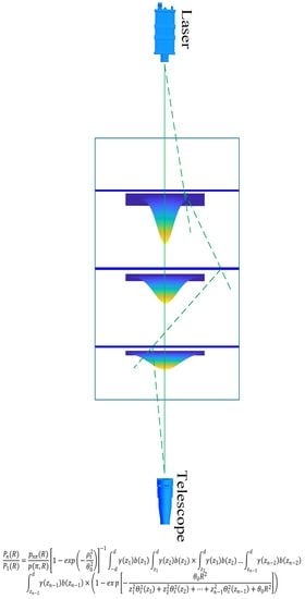
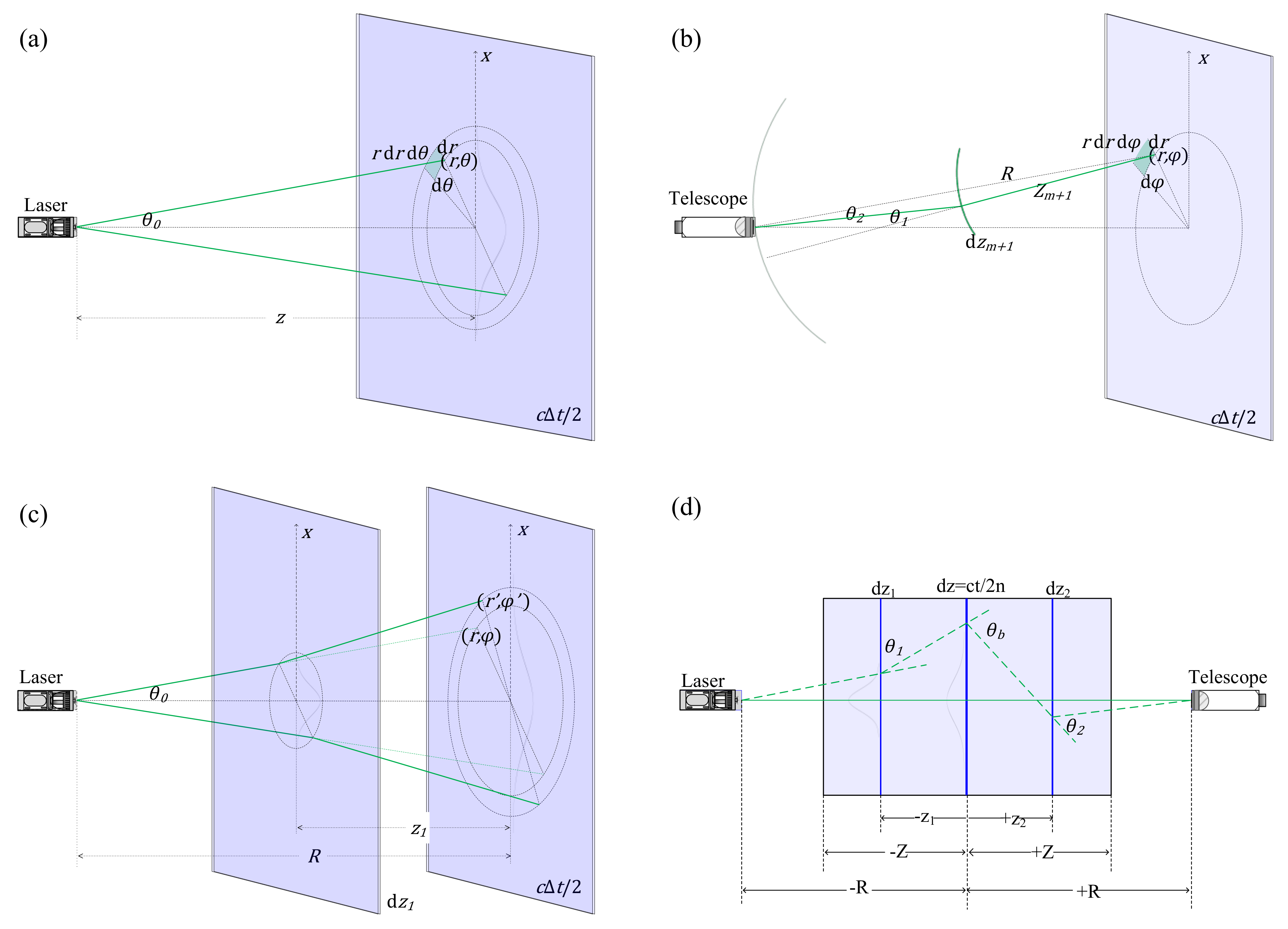
2.1. Multiple-Scattering Solution Based on QSAA

As depicted in Figure 1, a laser beam is received by a detector after multiple scattering in the water, where scattering at small angles ${\theta }_i$ is dominant. Under the framework of the quasi-single-scattering small-angle approximation (QSAA) [26], the received power is mainly composed of the multiple forward scatterings at small angles and a single backscattering at a large angle of nearly 180°.

For a source located at a point with a radius vector $R_0$, the laser beam first propagates to a position $R$ towards the direction $\mathit{n}$ by multiple forward scattering. Then, the laser beam travels to a position $R^{\prime }$ in the direction $-{\mathit{n}}^{\prime }$ after one large-angle backscattering at the position $\mathit{R}$ in the direction $-n_b$. Finally, the return signals are collected by the receiver at the position ${\mathit{R}}^{\prime }$. The echo signals are given by [27]:

$$\begin{gathered} P\left(R\right)=\int d{n}_b\int dnb\left(R\right)p_b\left(R;-n_b,n\right)\times \int d{R}_0\int d{\mathit{n}}_0{S}_{src}\left(R_0,n_0\right)G\left(R,n;R_0,n_0\right) \\ \times \int d{R}^{\prime }\int d{n}^{\prime }{S}_{rec}\left(R^{\prime },-n^{\prime }\right)G\left(R^{\prime },-n^{\prime };R,-n_b\right) \end{gathered}$$

(1)

where $S_{src}\left(R_0,n_0\right)$ is the normalized source radiance distribution with $\int d{R}_0\int d{n}_0{S}_{src}\left(R_0,n_0\right)=E_0$, $G\left(R,n;R_0,n_0\right)$ is the Green function for the radiative transfer equation, $b\left(\mathit{R}\right)$ is the scattering coefficient, $p_b\left(\mathit{R};-{\mathit{n}}_{\mathit{b}},\mathit{n}\right)$ is the scattering phase function (SPF) for the large backscattering angle ($-{\mathit{n}}_{\mathit{b}},\mathit{n}$) between vectors $\mathit{n}$ and $-{\mathit{n}}_{\mathit{b}}$, and $S_{rec}$ is receiver angular-spatial pattern of sensitivity.

Using the reciprocity principle that states $G\left(R^{\prime },-n^{\prime };R,-n_b\right)=G\left(R,n_b;R^{\prime },n^{\prime }\right)$ and defining the source and receiver-source radiances that describe the multiply scattered radiance at the point due to the true source $S_{src}$ and receiver-source $S_{src}^{rec}$, respectively,

$$I_{src}\left(R, n\right)=\int d{R}_0\int d{\mathit{n}}_0{S}_{src}\left(R_0,n_0\right)G\left(R,n;R_0,n_0\right)$$

(2)

$$I_{src}^{rec}\left(R, n\right)=\int d{R}_0\int d{\mathit{n}}_0{S}_{src}^{rec}\left(R_0,n_0\right)G\left(R,n;R_0,n_0\right)$$

(3)

where $S_{src}^{rec}\left(R^{\prime },n^{\prime }\right)=S_{rec}\left(R^{\prime },-n^{\prime }\right)$ is defined as a “receiver-source” which can be referred to as a radiance distribution of a fictitious source that is equivalent to the real receiver.

Then, we can obtain the echo signal power scattered at position $R$ of the form:

$$P\left(\mathit{R}\right)=\int d{n}_b\int dnb\left(R\right)p_b\left(R;-n_b,n\right)I_{src}\left(R, n\right)I_{src}^{rec}\left(R, n_b\right)$$

(4)

Equation (4) simplifies the complex lidar problem to two simple problems of light propagation that are connected by a single backscattering event.

For the light propagation problem in the conditions of QSAA, the solutions in the Fourier space are [28]:

$$\begin{gathered} {\tilde{I}}_{src}\left(z,\mathit{q},\mathit{p}\right)={\tilde{S}}_{src}\left(\mathit{q},\mathit{p}+\mathit{q}\mathit{z}\right)\tilde{G}\left(z,\mathit{q},\mathit{p}\right) \\ {\tilde{I}}_{src}^{rec}\left(z,\mathit{q},\mathit{p}\right)={\tilde{S}}_{src}^{rec}\left(\mathit{q},\mathit{p}+\mathit{q}\mathit{z}\right)\tilde{G}\left(z,\mathit{q},\mathit{p}\right) \\ \tilde{G}\left(z,\mathit{q},\mathit{p}\right)=\mathit{exp}\left({\int }_0^z-[c\left(z-\zeta \right)-b\left(z-\zeta \right)\tilde{p}\left(z-\zeta ,\mathit{p}+\mathit{q}\zeta \right)d\zeta \right) \end{gathered}$$

(5)

where the Fourier transforms have forms:

$$\begin{gathered} \tilde{I}\left(z,\mathit{q},\mathit{p}\right)={\int }_{-\infty }^{\infty }dr{\int }_{-\infty }^{\infty }d{n}_{\perp }I\left(z,\mathit{r},{\mathit{n}}_{\perp }\right)e^{\left(-i\mathit{q}\mathit{r}-ip{n}_{\perp }\right)} \\ {\tilde{S}}_{src}\left(\mathit{q},\mathit{p}\right)={\int }_{-\infty }^{\infty }dr{\int }_{-\infty }^{\infty }d{n}_{\perp }{S}_{src}\left(0,\mathit{r},{\mathit{n}}_{\perp }\right)e^{\left(-iqr-ip{n}_{\perp }\right)} \\ \tilde{p}\left(z,\mathit{p}\right)={\int }_{-\infty }^{\infty }d{n}_{\perp }p\left(z,{\mathit{n}}_{\perp }\right)e^{\left(-ip{n}_{\perp }\right)} \end{gathered}$$

(6)

where $\mathit{r}$ and $n_{\perp }$ are the projections of vectors $R$ and $n$ onto the plane z = constant, respectively. For the nearly backward scattering, the phase function $p_b\left(R;-n_b,n\right)$ depends on the difference $|n_{\perp }-n_{\perp b}|$ because of small angles of $n_{\perp }$ and $n_{\perp b}$. Here $p_b\left(z;-n_b,n\right)\approx p_b(z;\pi -|n_{\perp b}-n_{\perp }|)$. Substituting $n_{\perp }^{\prime }=n_{\perp b}-n_{\perp }$, Equation (4) can be rewritten as follows using SAA variables:

$$P\left(\mathit{z},r\right)=\int d{n}_{\perp }^{\prime }\int d{n}_{\perp }b\left(z\right)p_b\left(z;\pi -n_{\perp }^{\prime }\right)I_{src}\left(z,r,n_{\perp }\right)I_{src}^{rec}\left(z,r, n_{\perp }^{\prime }+n_{\perp }\right)$$

(7)

Integrating Equation (7) over $r$ in the plane $z$, the lidar return from depth $z$ is approximated as follows:

$$P\left(z\right)=\int dr\int d{n}_{\perp }\int d{n}_{\perp }^{\prime }b\left(\mathit{z}\right)p_b(z;\pi -|n_{\perp }^{\prime }|)I_{src}\left(\mathit{z},r,n_{\perp }\right)I_{src}^{rec}\left(\mathit{z},r, n_{\perp }^{\prime }+n_{\perp }\right)$$

(8)

Then, the integral from Equation (8) can be transformed into:

$$P\left(z\right)=\int d\mathit{r}\int d{\mathit{n}}_{\perp }^{\prime }\int d{\mathit{n}}_{\perp }b\left(z\right)p_b\left(z;\pi -\left|{\mathit{n}}_{\perp }^{\prime }\right|\right)S\left(z,r,n_{\perp }+n_{\perp d}\right)I^e\left(z,\mathit{r},{\mathit{n}}_{\perp }\right)$$

(9)

where $S\left(z,\mathit{r},{\mathit{n}}_{\perp }\right)$ is the true receiver function $S_{rec}\left(z,r,{\mathit{n}}_{\perp }\right)$, and $I^e\left(z,\mathit{r},{\mathit{n}}_{\perp }\right)$ is the effective radiance that is transmitted to the position ($z,\mathit{r}$) from the true source $S_{src}\left(0,\mathit{r},{\mathit{n}}_{\perp }\right)$ in the effective medium with optical parameters defined as follows:

$$c^e\left(z\right)=2c\left(z\right), b^e\left(z\right)=2b\left(z\right), p^e(z;\pi -|n_{\perp }^{\prime }|)=p(z;\pi -|n_{\perp }^{\prime }|)$$

(10)

2.2. Analytic Model Based on Convolutions of Gaussian Energy Density Functions

Equation (9) gives the general solution of return lidar signals, but it is still hard to use in practice. Here we derive a more practical model based on a Gaussian dependence of the transmitted laser beam on the divergence angle.

As shown in Figure 2a, for a source located at a point with a radius vector $R_0$, the number of incident photos $dN$ in the increment area $rdrd\phi$ on a slab of thickness $c\mathsf{\Delta }t/2$ at a distance $R$ without scattering is given by [29]:

$$dN=\frac{N_0}{\pi {\theta }_0^2{R}^2}\mathit{exp}\left(-\tau \left(R\right)\right)\mathit{exp}\left(-\frac{r^2}{{\theta }_0^2{R}^2}\right)rdrd\phi$$

(11)

where $N_0$ is the number of photos in the emitted pulse, ${\theta }_0$ is half of the divergence of the laser beam, $\tau \left(R\right)={{\displaystyle \int }}_0^{R}c\left(z^{\prime }\right)dz$ is the optical depth between the laser and the slab, and $c\left(z^{\prime }\right)$ is the beam attenuation coefficient as the function of $z$.

Photons arrive at the slab $c\mathsf{\Delta }t/2$ after a small-angle scattering event that occurs on the layer $d{z}_1$ at a distance $z_1$ from the slab $c\mathsf{\Delta }t/2$ (as shown in Figure 2c). If the scattering phase function is a Gaussian function of the scattering angle, the angle-spatial distribution of incident photons on the slab can be calculated as the convolution of the Gaussian laser beam with the Gaussian phase function, which has:

$$dN=\frac{\gamma \left(z_1\right)N_0}{\pi {\theta }_0^2{R}^2+\pi z_1^2{\mathsf{\Theta }}_s^2\left(z_1\right)}b\left(z_1\right)d{z}_1\mathit{exp}\left(-\tau \right)\mathit{exp}\left(-\frac{r^2}{{\theta }_0^2{R}^2+z_1^2{\mathsf{\Theta }}_s^2\left(z_1\right)}\right)rdrd\phi$$

(12)

where $\gamma \left(z\right)$ is the scattering energy in the forward peak of the scattering phase function at $z$ and is $\gamma \left(z\right)=\pi {\mathsf{\Theta }}_s^{2}p\left(0,z_1\right)/4\pi$, $p\left(\theta ,z_1\right)/4\pi$ is the scattering phase function at $z_1$, ${\mathsf{\Theta }}_s^2$ is the mean square angular width of the scattering phase function.

Then, consider photons incident on the slab after additional scatterings at distances $z_2,z_3,\dots ,z_m$ between $z_1$ and the slab. The number of incident photos $d{N}_m$ in the increment area $rdrd\phi$ on the slab after $m$ scattering can be calculated as the convolution of the Gaussian laser beam with m Gaussian phase functions, which has:

$$d{N}_m=N_t\frac{{{\displaystyle \prod }}_0^m\gamma \left(z_i\right)b\left(z_i\right)d{z}_i}{\pi {\theta }_0^2{R}^2+\pi {{\displaystyle \sum }}_0^m{z}_i^2{\Theta }_s^2\left(z_i\right)}\mathit{exp}\left(-\tau \right)\mathit{exp}\left(-\frac{r^2}{{\theta }_0^2{R}^2+{{\displaystyle \sum }}_0^m{z}_i^2{\Theta }_s^2\left(z_i\right)}\right)rdrd\phi$$

(13)

The beam backscattered from the area $rdrd\phi$ in the slab $c\mathsf{\Delta }t/2$ is collected by the receiver after an additional scattering at the layer $d{z}_{m+1}$ at distance $z_{m+1}$ is expressed as follows (Figure 2b):

$$\begin{array}{ll}\frac{d{N}_{m+1}}{dt}& =d{N}_m\frac{A_r}{R^2}\frac{p_{\pi n}\left(R\right)}{4\pi }b\left(R\right)\frac{c\mathsf{\Delta }t}{2}\frac{R^2\gamma \left(z_{m+1}\right)b\left(z_{m+1}\right)d{z}_1}{\pi z_{m+1}^2{\mathsf{\Theta }}_s^2\left(z_{m+1}\right)}\\ & \times \mathit{exp}\left(-\tau \right)\mathit{exp}\left(-\frac{{\theta }^2{R}^2}{z_{m+1}^2{\mathsf{\Theta }}_s^2\left(z_{m+1}\right)}\right)\theta d\theta d\varphi \end{array}$$

(14)

where $A_r$ is the area of the telescope, $\frac{p_{\pi n}\left(0\right)}{4\pi }$ is the average backscatter phase function near 180° for $n$th-order scattering, $b\left(R\right)$ is the scattering coefficient, $\theta$ is the angle between the beam path and the radius vector, and $\varphi$ is the angle of the radius vector.

Photons are collected by the receiver after additional scatterings at $z_{m+2},z_{m+3},\dots ,z_{n-1}$ between $z_{m+1}$ and the telescope, as shown in Figure 2d. The angular distribution of the photons can be calculated as the convolution of the Gaussian phase function, which has:

$$\begin{array}{ll}\frac{d{N}_n}{dt}& =d{N}_m\frac{A_r}{R^2}\frac{p_{\pi n}\left(R\right)}{4\pi }b\left(R\right)\frac{c\Delta t}{2}\frac{R^2{{\displaystyle \prod }}_{m+1}^{n-1}\gamma \left(z_i\right)b\left(z_i\right)d{z}_i}{\pi {{\displaystyle \sum }}_{m+1}^{n-1}{z}_i^2{\Theta }_s^2\left(z_i\right)}\\ & \times \mathit{exp}\left(-\tau \right)\times \mathit{exp}\left(-\frac{{\theta }^2{R}^2}{{{\displaystyle \sum }}_{m+1}^{n-1}{z}_i^2{\Theta }_s^2\left(z_i\right)}\right)\theta d\theta d\varphi \end{array}$$

(15)

After integrating over positions of the increment area $rdrd\phi$, the angular distributions of photons collected by a telescope can be expressed as follows:

$$\begin{array}{ll}\frac{d{N}_n}{dt}& =N_0\frac{A_r}{R^2}\frac{p_{\pi n}\left(R\right)}{4\pi }b\left(R\right)\frac{c\Delta t}{2}\frac{R^2{{\displaystyle \prod }}_0^{n-1}\gamma \left(z_i\right)b\left(z_i\right)d{z}_i}{\pi {\theta }_0^2{R}^2+\pi {{\displaystyle \sum }}_0^{n-1}{z}_i^2{\Theta }_s^2\left(z_i\right)}\times \mathit{exp}\left(-2\tau \right)\\ & \times \mathit{exp}\left(-\frac{{\theta }^2{R}^2}{{{\displaystyle \sum }}_{m+1}^{n-1}{z}_i^2{\Theta }_s^2\left(z_i\right)}\right)\rho d\rho d\varphi \end{array}$$

(16)

where $0<\rho <{\rho }_t$, and ${\rho }_t$ is half of the receiver FOV. Then, integrate over the FOV and divide by the signal scattering, which has:

$$\begin{array}{ll}\frac{d{P}_n\left(R\right)}{P_1\left(R\right)}=\frac{P_{\pi n}\left(0\right)}{P\left(\pi ,0\right)}& {\left[1-\mathit{exp}\left(-\frac{{\rho }_t^2}{{\theta }_0^2}\right)\right]}^{-1}{\Pi }_0^{n-1}\gamma \left(z_i\right)b\left(z_i\right)d{z}_i\\ & \times \left(1-\mathit{exp}\left(-\frac{{\rho }_t^2{R}^2}{{\theta }_0^2{R}^2+{\Sigma }_0^m{z}_i^2{\Theta }_s^2\left(x_i\right)}\right)\right)\end{array}$$

(17)

Finally, the ratio between the signal power of $n$th-order scattering and the signal-scattering can be calculated by integrating over $dz$ as follows:

$$\begin{array}{ll}\frac{P_n\left(R\right)}{P_1\left(R\right)}=\frac{P_{n\pi }\left(\mathrm{R}\right)}{P\left(\pi ,\mathrm{R}\right)}& {\left[1-\mathit{exp}\left(-\frac{{\rho }_t^2}{{\theta }_0^2}\right)\right]}^{-1}{\int }_{-d}^d\gamma \left(z_1\right)b\left(z_1\right){\int }_{z_1}^d\gamma \left(z_2\right)b\left(z_2\right)\\ & \times {\int }_{z_2}^d\gamma \left(z_3\right)b\left(z_2\right)\dots {\int }_{z_{n-3}}^d\gamma \left(z_{n-2}\right)b\left(z_{n-2}\right){\int }_{z_{n-2}}^d\gamma \left(z_{n-1}\right)b\left(z_{n-1}\right)\\ & \times (1-\mathit{exp}[-\frac{{\theta }_0{R}^2}{z_1^2{\Theta }_s^2\left(z_1\right)+z_2^2{\Theta }_s^2\left(z_2\right)+\dots +z_{n-1}^2{\Theta }_s^2{z}_{n-1}+{\theta }_0{R}^2}\left]\right)\end{array}$$

(18)

2.3. Sea Surface Modeling

The Cox and Munk sea surface probability distribution function [30,31] is used here to approximate wind-driven rough sea surface modeling:

$$p\left({\mu }_n,{\phi }_n\right)=\frac{1}{\pi {\sigma }^2{\mu }_n^3}\mathit{exp}\left(-\frac{1-{\mu }_n^2}{{\sigma }^2{\mu }_n^2}\right), {\sigma }^2=0.003+0.00512\times W$$

(19)

where ${\mu }_n=\cos \left({\theta }_n\right)$, ${\theta }_n$ is the polar angle, and ${\phi }_n$ is the azimuth angle for the wave facet normal vector $\overrightarrow{n}$. ${\sigma }^2$ is the variance as a function of the wind speed $W$ (m/s) above the sea surface.

The reflection $r\left({\mu }_0,{\phi }_0,{\mu }^{\prime },{\phi }^{\prime }\right)$ and transmission $t\left({\mu }_0,{\phi }_0,{\mu }^{\prime },{\phi }^{\prime }\right)$ function from direction (${\mu }_0,{\phi }_0$) towards (${\mu }^{\prime },{\phi }^{\prime }$) are expressed as follows (39):

$$r\left({\mu }_0,{\phi }_0,{\mu }^{\prime },{\phi }^{\prime }\right)=\frac{\pi p\left({\mu }_n,{\phi }_n\right)}{4\left|{\mu }_0\right|\left|{\mu }^{\prime }\right|{\mu }_n}{F}_r\left({\theta }_i\right)$$

(20)

$$t\left({\mu }_0,{\phi }_0,{\mu }^{\prime },{\phi }^{\prime }\right)=\frac{\pi p\left({\mu }_n,{\phi }_n\right)}{4\left|{\mu }_0\right|\left|{\mu }^{\prime }\right|{\mu }_n}{F}_t\left({\theta }_i\right)\frac{n_t^2\mathit{cos}{\theta }_t\mathit{cos}{\theta }_i }{{\left(n_t\mathit{cos}{\theta }_t-n_i\mathit{cos}{\theta }_i \right)}^2}$$

(21)

where $F_r\left({\theta }_i\right)$ and $F_t\left({\theta }_i\right)$ are Fresnel’s reflection and transmission coefficients, respectively.

3. Results

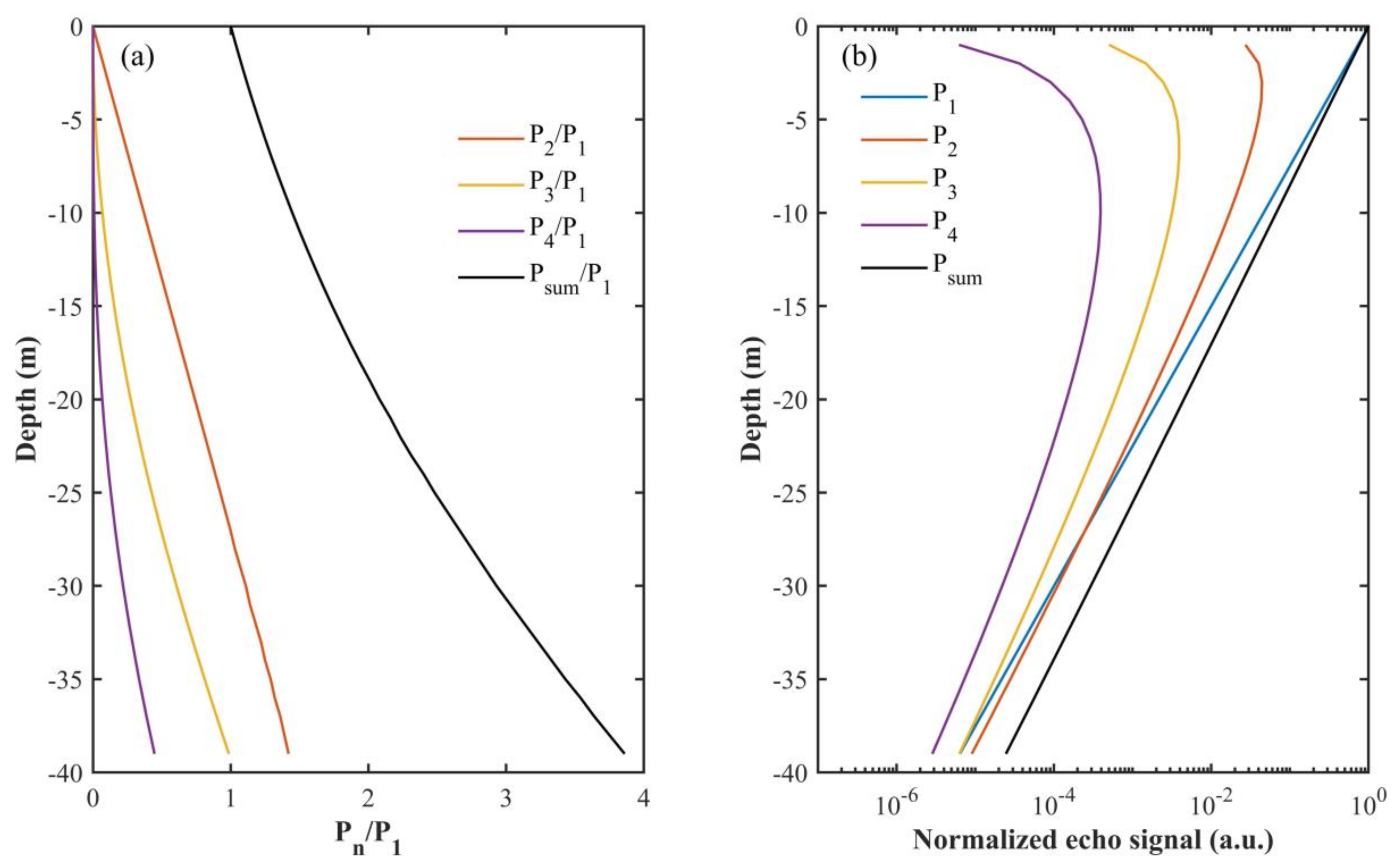
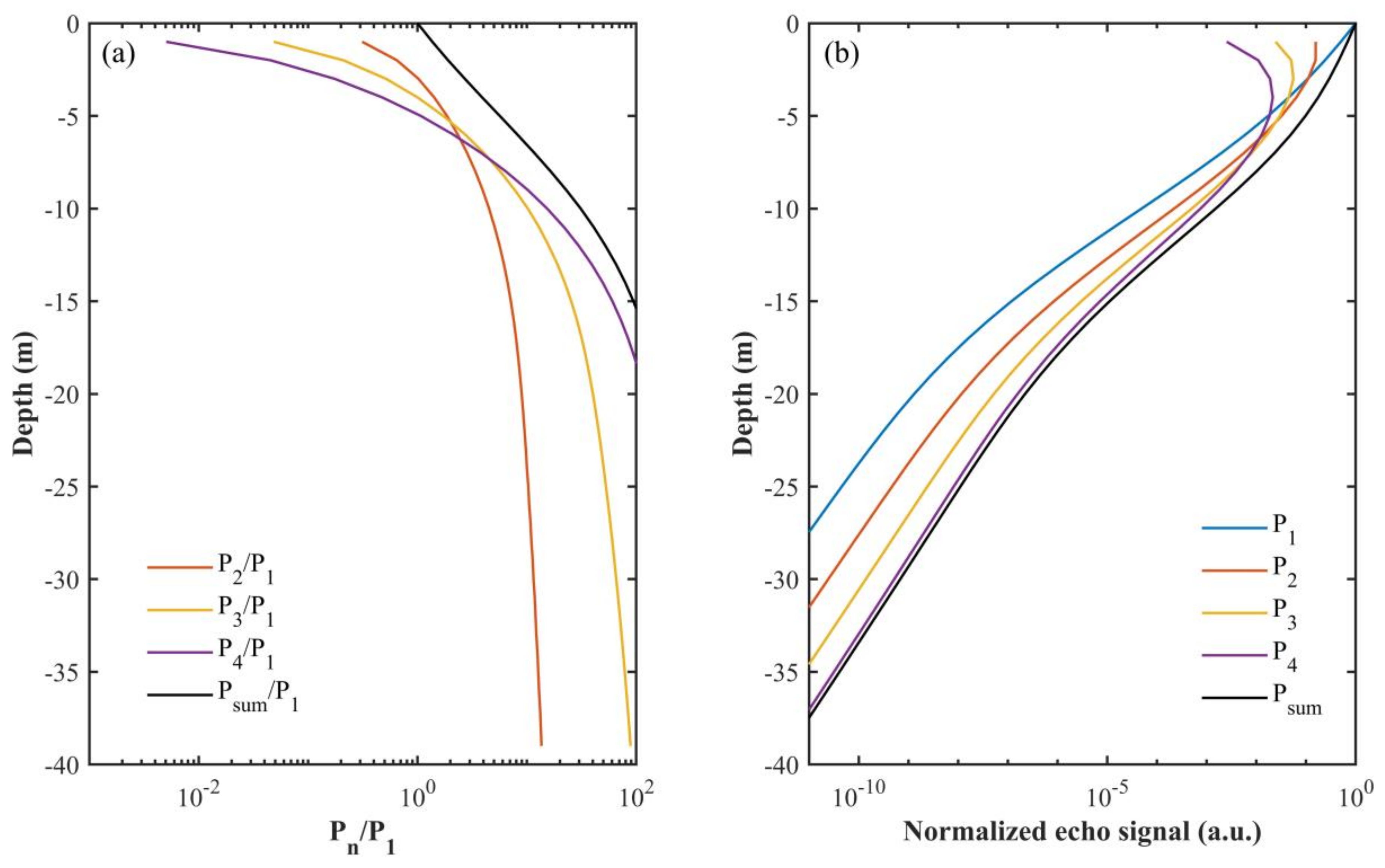
3.1. Effects of Multiple Scattering

Multiple scattering has a great influence on the lidar echo signals, so the effects of multiple scattering need to be determined for accurate lidar signal processing. To address the multiple scattering during lidar transmission, we simulated the ratios of double, three-order, and four-order scattering to single scattering, and their signal intensity is simulated, as well (Figure 3). The parameters of the lidar system used are $H =300 \mathrm{m}$, $\mathrm{FOV} =10 \mathrm{mrad}$, and the receiver aperture $\mathrm{Ar} =0.09{ \mathrm{m}}^2$. The water optical properties of clear ocean shown in

Table 1. Absorption and scattering coefficients for three typical types of seawater [32,33].

Water Types	$\mathit{a}\left({\mathbf{m}}^{-1}\right)$	$\mathit{b}\left({\mathbf{m}}^{-1}\right)$
Clear ocean	0.114	0.037
Coastal water	0.179	0.219
Turbid harbor	0.366	1.824

are used here. As shown in Figure 3, when the laser beam enters the water, the echo signal is dominated by single scattering, while the contribution of multiple scattering is negligible. However, multiple scattering signal increases with the propagation of laser beam in the water. In particular, when the depth exceeds 27 m, the double scattering signal begins to be more than single scattering signal, and at this depth range, the dominating backscattered signal received by the lidar FOV is multiple scattering. However, the total signal magnitude decreases as the depth increases because of water attenuation. Some backward signal exists out of the FOV after huge amounts of multiple scattering, which causes the decreasing of the signal magnitude as well. The difference between the total echo signals and the single scattering signal is shown in the result, and it increases with the propagation of the laser beam, which indicates that the multiple scattering effect is not negligible for lidar inversion.

3.2. Effects of Water Optical Property

To analyze the effects of different seawater optical properties, echo signals in three typical types of ocean water (Table 1) are simulated based on the same lidar system parameters as in Section 3.1. As shown in Figure 4, with the increases of water turbidity, the ratio of multiple scattering to single scattering becomes greater (Figure 4a–c). Meanwhile, due to the relatively high attenuation of the LiDAR signal with range, the lidar echo signal intensity in turbid water decreases faster, resulting in quite shallow penetration depth. Besides, the strong multiple scattering results in a more complex signal inversion. Therefore, a high signal-to-noise performance and an accurate inversion algorithm are needed for the detection of turbid water. The existent lidar inversion approaches and algorithms were often based on the solution form of the lidar equation with single scattering hypothesis. While multiple scattering leads to the estimated lidar attenuation coefficient value falling between the diffuse attenuation coefficient and the beam attenuation coefficient, the contribution of multiple scattering is considered as a hindrance for these algorithms. We still need to build a relationship between the estimated lidar attenuation coefficient and diffuse attenuation coefficient under different FOVs after solving the lidar equation with single scattering hypothesis. Hence, an improved multiple scattering lidar equation could be constructed and solved for higher accuracy based on a deeper understanding and a more accurate simulation of multiple scattering. The single-scattering lidar equation $S=A\beta (\pi )exp\left(-2K_{lidar}z\right)$ is then transformed to $S=A\beta (\pi )exp\left(-2K_{lidar}z\right)*F\left(z\right)$ [22]. F(z) represents multiple scattering effect function, which could be solved by the accurate simulation under different lidar conditions. We then could obtain the relationship between the estimated lidar attenuation coefficient and diffuse attenuation coefficient expressed as $K_{lidar}=K_d-\frac{1}{2z}lnF\left(z\right)$. Besides, accurate simulation of multiple scattering could be helpful for interpreting the depolarization introduced by multiple scattering, which in turn helps in the inversion of particles backscattering based on depolarization. In addition, simulation training data could be produced based on simulating under different water environment parameter conditions, then a signal matching algorithm (SMA) could be applied in the future, based on finding the proximate simulation signal compared to the measurement signal. This algorithm has the advantage of obtaining multiple water parameters simultaneously. A theoretical assessment of the stability of the algorithms to uncertainties could also be carried out. In addition, a tentative signal-to-noise (S/N) scheme for ocean lidar design which, comprehensively considering the inversion accuracy requirement, hardware cost, technical complexity, and so on, could be proposed based on a comprehensive lidar simulation system.

3.3. Validation

3.3.1. Validation under Extreme Condition

To validate the model, we simulated the results in extreme condition with a small FOV of 0.1 mrad. The used lidar system parameters are the same as those in Section 3.1 and the water type is the clear ocean. As shown in Figure 5, the multiple scattering signals are far below the single scattering, so the total scattering results meet with the single scattering results very well. The good agreement indicates the validity of the model.

3.3.2. Validation Using MC Model

Then, we used a semi-analytic MC model [17] to validate our simulation. Figure 6 represents the comparison results between our analytical model and MC simulation with several FOVs of 0.1 and 10 mrad under the same lidar system parameter settings as in Section 3.1. The MC model used a total of 10 million photons. The results show that our analytic results are in good agreement with the MC results, indicating the effectiveness of our model. The comparative statistical analysis between them is shown in

Table 2. Statistical analysis for comparison between our model and MC model.

FOV	R2	RMSE	MAD	MAPD
0.01 mrad	0.976	0.0132	0.0144	7.33%
10 mrad	0.985	0.0071	0.0057	4.78%

. The coefficient of determination (R²) is beyond 0.9, the mean absolute difference (MAD) is within 0.02, the root mean square error (RMSE) is within 0.02, and the mean absolute percent difference (MAPD) is within 8%, which indicates that our model works well for oceanographic lidar simulation.

3.3.3. Validation with In Situ Measurements

In situ measurement is used to validate the model. The data were collected at the station of $109.8164°\mathrm{E}, 18.3144°\mathrm{N}$ off Wuzhihzou Island on 30 September 2017, with the airborne oceanographic lidar designed by the Shanghai Institute of Optics and Fine Mechanics (SIOM), Chinese Academy of Sciences, Shanghai, China. The wavelength of 532 nm is used for oceanic detection, and the FOV is 6 mrad for shallow waters [7,10]. The water is quite clear, and the beam attenuation coefficient is less than 0.08 m⁻¹. The chlorophyll concentration is less than 0.17 mg/m³ and is nearly vertical homogeneous. The comparison result is shown in Figure 7. As the R² is 0.97, RMSE is 0.004, MAD is 0.004, and MAPD is 8.9%, our simulation result is in good agreement with the measurement, which indicates that our model works well for real ocean conditions.

4. Discussion

4.1. Effects of Multiple Scattering Contribution in Different FOVs

The results in Section 3.1 have shown the critical impact of multiple scattering on lidar return signals. Further analysis is needed to determine multiple scattering contributions in lidar echo signals with different FOVs to guide the lidar system design and inversion algorithms. Therefore, we simulated the multiple scattering under different FOVs in different seawater types based on the same lidar system parameters setting, as shown in Section 3.1. The water types used here are clear ocean and coastal water.

Figure 8 shows the results with FOVs of 10, 1, and 0.1 mrad in clear water. Figure 8a–d represent the double scattering, three-order scattering, four-order scattering, and the total echo signals, respectively. For a very small FOV of 0.1 mrad, the corresponding multiple scattering is so small that the total echo signal is mainly dominated by signal scattering. As the FOV increases, the multiple scattering increases, which leads to the result that the total echo signal decays more slowly with a larger FOV.

Figure 9 shows the results with FOVs of 10, 1, and 0.1 mrad in coastal water. For a small FOV (0.1 mrad), the single scattering signal contributes most of the total echo signal. Compared with the clear water shown in Figure 8, we find out the dependence of multiple scattering on water turbidity. For clear water, large FOV is good for obtaining multiple scattering signals due to less multiple scattering in clear ocean. However, smaller FOV is better for the single scattering signal for coastal water because of the stronger multiple scattering. Therefore, the water inherent optical properties should be taken into account when it comes to the FOV design for a lidar system. A multiple-FOV or adjustable-FOV lidar system configuration will be a good choice for signal inversion.

4.2. Effects of SPF

To analyze the effects of different SPFs, we simulated the lidar echo signal using HG (g = 0.924), FF, TTHG, and Petzold SPFs with the same lidar system parameters as in Section 3.1. As shown in Figure 10b, FF simulation results agree with Petzold results very well as the result of a great match of their SPFs (red and purple lines in Figure 10a). However, the results of HG are slightly smaller. It is largely because HG SPF has a much smaller backscatter at a large scattering angle, as shown in Figure 10a, which is caused by the sharp forward peaks of the seawater phase function [26]. Relatively, the results of TTHG are much higher than the others due to its higher backscatter, as shown in Figure 10a. Therefore, the real oceanic SPF should be taken into account during lidar simulation.

4.3. Effects of Wind Speed

Wind exerts a subtle influence on lidar echo by changing the roughness of the sea surface. To determine effects of wind speed, we computed lidar beam reflectivity and transmissivity with different wind speeds, considering four cases when laser beam propagates through the sea surface: laser beam reflected from the air towards air (RAA); beam reflected from the water towards water (RWW); beam transmitted from air into water (TAW); beam transmitted from water into air (TWA). The results are shown in Figure 10. When the laser beam propagates from the air (Figure 11a,b), the light reflectivity changes slowly within a small laser incident angle of 30°. Then, it increases rapidly with the increase of laser incident angle. Meanwhile, the transmissivity is, oppositely, on the decrease. The wind tends to improve the transmission of the laser. In other words, higher wind speed leads to greater transmissivity and less reflectivity. When a laser beam propagates from water (Figure 11c,d), the light reflectivity increases, while the transmissivity is on the decrease with the increase of the incident angle. When the incident angle exceeds the critical angle of total reflection, all light is reflected from water to water totally, and the critical angle increases with the increase of wind speed. The result indicates that the impact of wind-driven rough sea surface on laser transmission through the air–sea interface can be neglected in small incident angles (Figure 11b) to simplify the simulation. Although the Cox and Munk model has been widely used to simulate rough sea surface in ocean color remote sensing [17,34,35], it is obtained for wind speeds of 1–14 m/s and cannot produce wave elevations [36]. Cox–Munk simulates capillarity waves but ignores gravity waves. A more accurate sea surface model considering the shadowing effect [37] will be modified for oceanic lidar simulation in the future. As the Cox and Munk model is for isotropic sea surface, other anisotropic surfaces [38] are used to modify our model. One notes that because the scattering phase function is difficult to determine accurately, the simulation accuracy may be reduced in a complex oceanic environment. The wide-angle scattering occurs in the dense subsurface phytoplankton, which sometimes makes it hard to use this model, and the pulse stretching is included in this model.

4.4. Effects of Stratified Water

We analyzed the effects of stratified water that are simulated by using the chlorophyll Gaussian profile [39]. The vertical structure of chlorophyll concentration affects the echo signal by changing the water optical properties, including attenuation and scattering coefficients. The chlorophyll profile $Chl\left(z\right) \left(\mathrm{m}\mathrm{g}·{\mathrm{m}}^3\right)$ is expressed by Gaussian function as follows:

$$Chl\left(z\right)=C_1+C_0\mathit{exp}\left(-\frac{{\left(z-z_{max}\right)}^2}{2{\sigma }_c^2}\right)$$

(22)

where $C_0$ is chlorophyll concentration $\left(\mathrm{m}\mathrm{g}·{\mathrm{m}}^3\right)$ at the sea surface, $C_1$ is the constant background phytoplankton biomass $\left(\mathrm{m}\mathrm{g}·{\mathrm{m}}^3\right)$, $z_{max}$ is the depth where the maximum Gaussian chlorophyll value is reached, and ${\sigma }_c$ is the width of the chlorophyll peak. The parameters used here are $C_0=1 \mathrm{m}\mathrm{g}·{\mathrm{m}}^3,C_1=0.5 \mathrm{m}\mathrm{g}·{\mathrm{m}}^3,z_{max}=10 \mathrm{m},{\mathsf{\sigma }}_c=5 \mathrm{m}$.

Figure 12 shows the simulation results of stratified water. Compared with results of homogeneous water, which represent a linear decay in the logarithm coordinates as shown in Figure 3b, the echo signal in stratified water has a bulge at the depth of 10 m where the maximum Gaussian chlorophyll value is reached. Therefore, the subsurface chlorophyll maximum layer can be detected by using the bulge of lidar measurements [12,40]. Besides, the multiple scattering occurs more frequently, as shown in Figure 12a. Considering the worldwide stratification in the real marine environment, stratified water is supposed to be considered in lidar simulation.

4.5. Effects of Particle Sizes

Figure 13 represents the ratio of total echo signal to single scattering with different particle radiuses. The lidar system parameters are the same as those in Section 3.1. The results show that particle sizes have a vital influence on multiple scattering of lidar. With a very small particle radius ($0.1 \mathsf{\mu }\mathrm{m}$), the ratio of total echo signal magnitude to single scattering is close to 1 at all depths, which means that the return signal is mainly dominated by single scattering, and multiple scattering does not increase with the propagation of the laser beam. When particle radius is greater, multiple scattering increases and plays a major role in the total signal. Considering the complexity of particulates in the ocean, the real particle radius should be taken into account during lidar simulation. Besides, this feature can be used for the retrieval of particulate sizes in water.

5. Conclusions

We introduced a novel, fast multiple-scattering approximate model for ocean lidar. Preliminary results indicate that it works well for oceanic lidar simulation of beam transmission in the air–sea coupled systems with a wind-driven rough sea surface. Compared with previous analytic models, our model can deal with stratified water, and it can be applied to arbitrary SPFs. However, because the scattering phase function is difficult to determine accurately in complex turbid oceanic water, the wide-angle scattering occurring in the strong scattering layer also makes it hard to use this model, and the pulse stretching is not included in this model. The results show that multiple scattering signal increases with the propagation of the laser beam in the water. The ratio of multiple scattering to single scattering becomes greater with the increase of water turbidity. However, the total signal intensity decreases with the increase of the depth because of water attenuation and decreases faster, especially in turbid water. Thus, the penetration in turbid water is rather shallow. Besides, the strong multiple scattering results in a more complex signal inversion. A good agreement between our model and the MC simulation demonstrates its validation. Their coefficient of determination is beyond 0.9, the RMSE is within 0.02, the MAD is within 0.02, and the MAPD is within 8%, which indicates that our model works well for oceanographic lidar simulation. Besides, the validation with measurement also demonstrates its efficiency in real oceanic water.

Different FOVs were used to estimate their impact on multiple scattering. For a small FOV of 0.1 mrad, multiple scattering is so small that the total echo signal is mainly dominated by single scattering. For larger FOVs, the multiple scattering is more critical for the total signal. Simulation results with different SPFs show that the widely used HG SPF has poor performance at small or large scattering angles. Therefore, using the real oceanic SPF for the lidar simulation will improve its accuracy. A corresponding bulge appears in the simulation with stratified water, and it can be used for SCML detection. Different particle radiuses were applied to analyze their influence on lidar transmission. For a very small particle radius (0.1 $\mathsf{\mu }\mathrm{m}$), the multiple scattering is so small that it is negligible; thus, we can only consider the single scattering. For a larger particle radius, the total signal is dominated by multiple scattering.

Overall, multifactor influences including stratified water, SPF, and particular size were analyzed in our simulation, which shows that they are not negligible. These results are expected to provide a reference to the design of the oceanographic lidar system and contribute to the processing of lidar echo signals.

References

1. Dickey, T.; Lewis, M.; Chang, G. Optical oceanography: Recent advances and future directions using global remote sensing and in situ observations. Rev. Geophys. 2006, 44. [Google Scholar] [CrossRef] [Green Version]
2. Liu, H.; Chen, P.; Mao, Z.; Pan, D. Iterative retrieval method for ocean attenuation profiles measured by airborne lidar. Appl. Opt. 2020, 59, C42–C51. [Google Scholar] [CrossRef]
3. Behrenfeld, M.J.; Boss, E. Beam attenuation and chlorophyll concentration as alternative optical indices of phytoplankton biomass. J. Mar. Res. 2006, 64, 431–451. [Google Scholar] [CrossRef]
4. Hostetler, C.A.; Behrenfeld, M.J.; Hu, Y.; Hair, J.W.; Schulien, J.A. Spaceborne Lidar in the Study of Marine Systems. Ann. Rev. Mar. Sci. 2018, 10, 121–147. [Google Scholar] [CrossRef] [PubMed] [Green Version]
5. Churnside, J.H. Review of profiling oceanographic lidar. Opt. Eng. 2014, 53, 051405. [Google Scholar] [CrossRef] [Green Version]
6. Chen, P.; Jamet, C.; Zhang, Z.; He, Y.; Mao, Z.; Pan, D.; Wang, T.; Liu, D.; Yuan, D. Vertical distribution of subsurface phytoplankton layer in South China Sea using airborne lidar. Remote Sens. Environ. 2021, 263, 112567. [Google Scholar] [CrossRef]
7. Liu, H.; Chen, P.; Mao, Z.; Pan, D.; He, Y. Subsurface plankton layers observed from airborne lidar in Sanya Bay, South China Sea. Opt. Express 2018, 26, 29134–29147. [Google Scholar] [CrossRef]
8. Churnside, J.H.; Marchbanks, R.D. Subsurface plankton layers in the Arctic Ocean. Geophys. Res. Lett. 2015, 42, 4896–4902. [Google Scholar] [CrossRef]
9. Churnside, J.H.; Donaghay, P.L. Thin scattering layers observed by airborne lidar. ICES J. Mar. Sci. 2009, 66, 778–789. [Google Scholar] [CrossRef]
10. Chen, P.; Pan, D. Ocean Optical Profiling in South China Sea Using Airborne LiDAR. Remote Sens. 2019, 11, 1826. [Google Scholar] [CrossRef] [Green Version]
11. Churnside, J.; Hair, J.; Hostetler, C.; Scarino, A. Ocean Backscatter Profiling Using High-Spectral-Resolution Lidar and a Perturbation Retrieval. Remote Sens. 2018, 10, 2003. [Google Scholar] [CrossRef] [Green Version]
12. Churnside, J.H.; Marchbanks, R.D. Inversion of oceanographic profiling lidars by a perturbation to a linear regression. Appl. Opt. 2017, 56, 5228–5233. [Google Scholar] [CrossRef] [PubMed]
13. Jamet, C.; Ibrahim, A.; Ahmad, Z.; Angelini, F.; Babin, M.; Behrenfeld, M.J.; Boss, E.; Cairns, B.; Churnside, J.; Chowdhary, J.; et al. Going Beyond Standard Ocean Color Observations: Lidar and Polarimetry. Front. Mar. Sci. 2019, 6, 251. [Google Scholar] [CrossRef]
14. Zhou, Y.; Chen, W.; Cui, X.; Malinka, A.; Liu, Q.; Han, B.; Wang, X.; Zhuo, W.; Che, H.; Song, Q.; et al. Validation of the Analytical Model of Oceanic Lidar Returns: Comparisons with Monte Carlo Simulations and Experimental Results. Remote Sens. 2019, 11, 1870. [Google Scholar] [CrossRef] [Green Version]
15. Ramella-Roman, J.; Prahl, S.; Jacques, S. Three Monte Carlo programs of polarized light transport into scattering media: Part I. Opt. Express 2005, 13, 4420–4438. [Google Scholar] [CrossRef] [PubMed]
16. Gordon, H.R. Interpretation of airborne oceanic lidar: Effects of multiple scattering. Appl. Opt. 1982, 21, 2996. [Google Scholar] [CrossRef] [PubMed]
17. Chen, P.; Jamet, C.; Mao, Z.; Pan, D. OLE: A Novel Oceanic Lidar Emulator. IEEE Trans. Geosci. Remote Sens. 2020, 1–15. [Google Scholar] [CrossRef]
18. Liu, Q.; Cui, X.; Chen, W.; Liu, C.; Bai, J.; Zhang, Y.; Zhou, Y.; Liu, Z.; Xu, P.; Che, H.; et al. A semianalytic Monte Carlo radiative transfer model for polarized oceanic lidar: Experiment-based comparisons and multiple scattering effects analyses. J. Quant. Spectrosc. Radiat. Transf. 2019, 237, 106638. [Google Scholar] [CrossRef]
19. Liu, D.; Chen, P.; Che, H.; Liu, Z.; Liu, Q.; Song, Q.; Chen, S.; Xu, P.; Zhou, Y.; Chen, W.; et al. Lidar Remote Sensing of Seawater Optical Properties: Experiment and Monte Carlo Simulation. IEEE Trans. Geosci. Remote Sens. 2019, 57, 9489–9498. [Google Scholar] [CrossRef]
20. Chen, P.; Pan, D.; Mao, Z.; Liu, H. Semi-analytic Monte Carlo radiative transfer model of laser propagation in inhomogeneous sea water within subsurface plankton layer. Opt. Laser Technol. 2019, 111, 1–5. [Google Scholar] [CrossRef]
21. Kim, M.; Kopilevich, Y.; Feygels, V.; Park, J.Y.; Wozencraft, J. Modeling of Airborne Bathymetric Lidar Waveforms. J. Coast. Res. 2016, 76, 18–30. [Google Scholar] [CrossRef] [Green Version]
22. Kopilevich, Y.I.; Surkov, A.G. Mathematical modeling of the input signals of oceanological lidars. J. Opt. Technol. 2008, 75, 321–326. [Google Scholar] [CrossRef]
23. Malinka, A.V.; Zege, E.P. Analytical modeling of Raman lidar return, including multiple scattering. Appl. Opt. 2003, 42, 1075–1081. [Google Scholar] [CrossRef] [PubMed]
24. Kopilevich, Y.; Feygels, V.; Surkov, A. Mathematical Modeling of Input Signals for Oceanographic Lidar Systems; SPIE: Bellingham, WA, USA, 2003; Volume 5155. [Google Scholar]
25. Walker, R.E.; McLean, J.W. Lidar equations for turbid media with pulse stretching. Appl. Opt. 1999, 38, 2384–2397. [Google Scholar] [CrossRef]
26. Katsev, I.L.; Zege, E.P.; Prikhach, A.S.; Polonsky, I.N. Efficient technique to determine backscattered light power for various atmospheric and oceanic sounding and imaging systems. J. Opt. Soc. Am. A 1997, 14, 1338. [Google Scholar] [CrossRef]
27. Weitkamp, C. Lidar: Range-Resolved Optical Remote Sensing of the Atmosphere; Springer Science & Business: Berlin/Heidelberg, Germany, 2006; Volume 102. [Google Scholar]
28. Ishimaru, A. Wave Propagation and Scattering in Random Media; Academic Press: Cambridge, MA, USA, 1978; Volume 2. [Google Scholar]
29. Eloranta, E.W. Practical model for the calculation of multiply scattered lidar returns. Appl. Opt. 1998, 37, 2464–2472. [Google Scholar] [CrossRef]
30. Cox, C.; Munk, W. Statistics of the sea surface derived from Sun glitter. J. Mar. Res. 1954, 13, 198–227. [Google Scholar]
31. Cox, C.; Munk, W. Measurement of the Roughness of the Sea Surface from Photographs of the Sun’s Glitter. J. Opt. Soc. Am. 1954, 44, 838–850. [Google Scholar] [CrossRef]
32. Gabriel, C.; Khalighi, M.-A.; Bourennane, S.; Léon, P.; Rigaud, V. Monte-Carlo-Based Channel Characterization for Underwater Optical Communication Systems. J. Opt. Commun. Netw. 2013, 5, 1–12. [Google Scholar] [CrossRef] [Green Version]
33. Mobley, C.D.; Mobley, C.D.; Preisendorfer, R.W. Light and Water: Radiative Transfer in Natural Waters; Academic Press: Cambridge, MA, USA, 1994. [Google Scholar]
34. Zhai, P.-W.; Hu, Y.; Chowdhary, J.; Trepte, C.R.; Lucker, P.L.; Josset, D.B. A vector radiative transfer model for coupled atmosphere and ocean systems with a rough interface. J. Quant. Spectrosc. Radiat. Transf. 2010, 111, 1025–1040. [Google Scholar] [CrossRef]
35. Chami, M.; Lafrance, B.; Fougnie, B.; Chowdhary, J.; Harmel, T.; Waquet, F. OSOAA: A vector radiative transfer model of coupled atmosphere-ocean system for a rough sea surface application to the estimates of the directional variations of the water leaving reflectance to better process multi-angular satellite sensors data over the ocean. Opt. Express 2015, 23, 27829–27852. [Google Scholar] [CrossRef] [PubMed] [Green Version]
36. Mobley, C.D. Polarized reflectance and transmittance properties of windblown sea surfaces. Appl. Opt. 2015, 54, 4828–4849. [Google Scholar] [CrossRef] [PubMed]
37. Ross, V.; Dion, D.; Potvin, G. Detailed analytical approach to the Gaussian surface bidirectional reflectance distribution function specular component applied to the sea surface. J. Opt. Soc. Am. A Opt. Image Sci. Vis. 2005, 22, 2442–2453. [Google Scholar] [CrossRef] [PubMed]
38. Ramon, D.; Steinmetz, F.; Jolivet, D.; Compiègne, M.; Frouin, R. Modeling polarized radiative transfer in the ocean-atmosphere system with the GPU-accelerated SMART-G Monte Carlo code. J. Quant. Spectrosc. Radiat. Transf. 2019, 222, 89–107. [Google Scholar] [CrossRef]
39. Muñoz-Anderson, M.; Millán-Núñez, R.; Hernández-Walls, R.; González-Silvera, A.; Santamaría-del-Ángel, E.; Rojas-Mayoral, E.; Galindo-Bect, S. Fitting vertical chlorophyll profiles in the California Current using two Gaussian curves. Limnol. Oceanogr. Methods 2015, 13, 416–424. [Google Scholar] [CrossRef]
40. Chen, P.; Mao, Z.; Zhang, Z.; Liu, H.; Pan, D. Detecting subsurface phytoplankton layer in Qiandao Lake using shipborne lidar. Opt. Express 2020, 28, 558–569. [Google Scholar] [CrossRef]
Figure 1. The geometry of multiple scattering of lidar propagation. 2 Θ is full-angle receiver field of view (FOV); θ i is forward scattering angle; θ b is backscattering angle; Θ and D are half-angle receiver field of view and position of the “equivalent” lidar system due to refraction.
Remotesensing 13 03677 g001
Figure 2. The geometry of lidar propagation. (a) Trajectory of a photon transmitted to the slab without scattering; (c) trajectory of a photon forward-scattered at a distance z 1 ; (b) trajectory of a photon propagating back to the telescope after back-scattering at the slab; (d) the unfolded multiple-scattering geometry of the lidar return.
Remotesensing 13 03677 g002
Figure 3. Effects of multiple scattering on lidar echo signal. (a) The ratios of double, three-order, and four-order scattering to single scattering; (b) the single scattering, double scattering, three-order, and four scattering echo signal intensity.
Remotesensing 13 03677 g003
Figure 4. Effects of different water optical properties. (a) The ratio of double scattering to single scattering; (b) the ratio of three-order scattering to single scattering; (c) the ratio of four-order scattering to single scattering; (d) the total echo signals with different water optical properties.
Remotesensing 13 03677 g004
Figure 5. The results with FOV of 0.1 mrad. (a) The ratios of double and three-order scattering to single scattering; (b) the single, double, three-order scattering, and total echo signals magnitude.
Remotesensing 13 03677 g005
Figure 6. Comparison between our analytic model and MC model with FOVs of 10 mrad (a) and 0.1 mrad (b).
Remotesensing 13 03677 g006
Figure 7. Comparison between our analytic model and in situ measurement.
Remotesensing 13 03677 g007
Figure 8. Lidar multiple scattering under different FOVs in open ocean water. (a) Double scattering signal; (b) three-order scattering signal; (c) four-order scattering; (d) the total echo signals.
Remotesensing 13 03677 g008
Figure 9. Lidar multiple scattering under different FOVs in coastal water. (a) Double scattering signal; (b) three-order scattering signal; (c) four-order scattering; (d) the total echo signals.
Remotesensing 13 03677 g009
Figure 10. Effects of SPFs. (a) SPFs’ dependency on scattering angles; (b) simulated echo signals with these SPFs.
Remotesensing 13 03677 g010
Figure 11. Effects of the wind-driven rough sea surface. (a) The reflectivity of RAA; (b) the transmissivity of TAW; (c) the reflectivity of RWW; (d) the transmissivity of TWA.
Remotesensing 13 03677 g011
Figure 12. Effects of stratified seawater. (a) The ratios of double, three-order, and four-order scattering to single scattering; (b) the single, double, three-order, and four-order scattering, and total echo signals.
Remotesensing 13 03677 g012
Figure 13. Effects of particulate sizes.
Remotesensing 13 03677 g013