Locating Charcoal Production Sites in Sweden Using LiDAR, Hydrological Algorithms, and Deep Learning

Abstract

Over the past several centuries, the iron industry played a central role in the economy of Sweden and much of northern Europe. A crucial component of iron manufacturing was the production of charcoal, which was often created in charcoal piles. These features are visible in LiDAR (light detection and ranging) datasets. These charcoal piles vary in their morphology by region, and training data for some feature types are severely lacking. Here, we investigate the potential for machine automation to aid archaeologists in recording charcoal piles with limited training data availability in a forested region of Jönköping County, Sweden. We first use hydrological depression algorithms to conduct a preliminary assessment of the study region and compile suitable training data for charcoal production sites. Then, we use these datasets to train a series of RetinaNet deep learning models, which are less computationally expensive than many popular deep learning architectures (e.g., R-CNNs), allowing for greater usability. Together, our results demonstrate how charcoal piles can be automatically extracted from LiDAR datasets, which has great implications for improving our understanding of the long-term environmental impact of the iron industry across Northern Europe. Furthermore, our workflow for developing and implementing deep learning models for archaeological research can expand the use of such methods to regions that lack suitable training data.

1. Introduction

Over the last 2500 years, iron production has been a central economic industry in Sweden [1,2,3,4]. During the 17th century, there was a drastic increase in iron production that coincided with the immigration of Walloons, who brought new finery processes that produced a type of wrought iron known as iron rod, as well as new charcoal production and forestry techniques [5]. By the 16th and 17th centuries, production was accelerated by capitalist ventures and continued well into the 19th century [6], so much so that by the 18th century, iron production made up three quarters of Sweden’s total exports [7]. During this period, the cost of charcoal has been estimated to have made up more than 50 percent of the production costs for wrought iron. As a result of major alterations in the structure of the iron industry, charcoal use decreased from the mid-19th century, when many of the small foundries were closed, and larger foundries were endorsed. Moreover, black coal was used to a higher degree, due to its higher energy content [5].

To understand the iron production industry in this region, knowledge of charcoal manufacturing is essential. To produce charcoal from wood, slow combustion and a controlled supply of oxygen is required. This is achieved through different types of constructions, either sunken (pits) or above ground (piles) [4]. These constructions are called charcoal pits, which date to between the late Iron Age through the Medieval Period, or charcoal piles that emerged in the post-Medieval Period around the 12th century [4,5,8]. The exact morphological characteristics vary by local tradition, but most are defined by a pile of wood covered in turf and surrounded by post-holes where supporting structures were placed around burning materials [5]. Charcoal piles were produced across much of Europe and display morphologies that range in similarity to those in Sweden (e.g., [9,10]). This means that attempts to automate their detection can have far-reaching implications for archaeologists working beyond Sweden and for studies attempting to understand cultural affiliation of land use activity in given localities.

However, current information about the regional morphological diversity of charcoal piles in Sweden is somewhat limited, even though there are more than 50,000 charcoal production sites registered in the Swedish National Heritage Board’s database for archaeological sites and monuments. This is due to several different factors. Typologically, charcoal production sites can vary in shape and size depending on time and place of origin, but often share basic characteristics (such as material composition and a distinctive topographic signature from the surrounding environment). There are also local types that differ from the traditional classes. Therefore, despite large numbers of recorded charcoal production sites, these records do not contain information on many local charcoal production typologies.

Further limitations to knowledge of Sweden’s charcoal piles come from problematic elements associated with obtaining accurate radiometric dates from these particular sites. Radiocarbon (¹⁴C) analyses are limited to providing rough estimates, as many charcoal production sites were in use for long periods of time using long-growth species. Even if the individual phases of a pit could be distinguished by applying a correct excavation method, the dates obtained from a ¹⁴C analysis would not meet chronometric hygiene standards [11]. While wood-powered charcoal piles should, theoretically, be datable using dendrochronology, the species of trees used in the piles were often short-lived and rarely old enough to provide acceptable dates [5]. Taking these aspects into consideration, it is currently difficult to typologize and make any developmental patterns salient.

Charcoal production sites (sometimes referred to as relict charcoal hearths [RCHs]) are studied across Europe and North America, increasingly via LiDAR and LiDAR-derived products (e.g., [12,13,14,15]). RCHs provide key insight not only to past economic activities, but also the environmental impacts of industrialization in Europe and the United States, where charcoal and iron production were central industries [13,16,17,18]. Many of these RCHs are located deep within forests, and thus LiDAR has aided in their detection at increasing rates over the past decade. This study hopes to contribute to this broadening literature to improve the ability of archaeologists to document charcoal production sites and better understand their role in socioenvironmental and ecological systems.

Here, we investigate the capacity for automated remote sensing methods and LiDAR data to identify a specific type of charcoal pile known in Swedish as resmila, which directly translates to “erected charcoal pile”. Resmila were constructed by placing firewood vertically leaning towards a central log (Figure 1). In certain cases, a foundation below the firewood is also constructed in order to regulate the influx of oxygen from the ground. The diameter of a standard erect charcoal pile was commonly between ten and fifteen meters [5].

Within Jönköping County, Sweden, the documentation of resmila in the National Database is limited, as only a handful were previously discovered in large part due to the difficulty in identifying them during ground surveys. As such, we developed an iterative approach for deploying advanced machine intelligence techniques in regions where information about these features is lacking (Figure 2). Thus, our case study has implications for archaeologists around the world where automated site prospection is hampered by limited available training datasets. Particularly among studies of RCHs in Europe and North America, our methods can aid in the documentation of broad landscapes under tree canopies where these features are often abundant but poorly recognized on a landscape scale [13]. Using depression algorithms, we can (1) allow for relatively good initial assessment of certain archaeological features, identifying dozens to hundreds of these deposits. This then permits for (2) the detection of initial training datasets needed for the implementation of more sophisticated automation algorithms, such as deep learning. In what follows, we provide a case study from a 22 km² area of Jönköping County, Sweden, where charcoal piles were recently located by one of the authors (JL) by manually evaluating LiDAR data (Figure 3).

2. Automation in Archaeological Remote Sensing

Machine learning and computer automation applications have advanced rapidly in the past two decades [20,21,22]. The methods applied for automated feature detection are widely varied, especially for landscape-scale datasets such as LiDAR and satellite imagery [23,24,25,26,27]. Among the many advances made by scholars in the past few years, the use of morphological characteristics and object-based classifiers has been widely applied, especially to LiDAR data (see [13]). More recently, developments in deep learning (DL) have made progress in improving the accuracy of automated prospection of archaeological materials (e.g., [17]).

DL is a branch of artificial intelligence (AI) that has been recently gaining popularity among computational archaeologists [24,28,29,30,31]. DL has resulted in higher accuracy by increasing true positives while reducing false positive results compared to other machine learning and automation techniques [24,32,33]. Convolutional Neural Networks (CNN’s), specifically, are a type of DL architecture that have led the charge in archaeological applications. CNNs input data from multidimensional matrices, which allow them to quantify patterns using neighboring pixels, which can affect the final identification [24,31]. As such, CNNs are often more sensitive to subtle patterns within datasets than other forms of machine learning.

DL applications, while now growing rapidly, have remained limited within archaeology, largely because of the computational power, amount of training data, and expertise required to successfully develop these models [34]. The need for large training datasets has been substantially reduced by transfer learning (e.g., [24]), which is a technique that uses previously trained DL models to train new (oftentimes unrelated) models [35]. Transfer learning has led to a breakthrough in archaeological research [32].

Within DL, there are two main architectural types for models: two-stage and one-stage. Two-stage detectors have been more popular among archaeologists, particularly those studying landscape scale datasets [29,36] because they often achieve greater accuracy than one-stage detectors. This stems from the ability of two-stage detectors to reduce false positives by using their two-stages to generate potential feature maps while simultaneously filtering out negative locations [37]. Two-stage detectors are computationally intensive, however, making their use more limited to those with high-computing power. Single stage detectors, in contrast, require less computational power but have historically struggled with reducing background noise, leading to lower performance. However, recent developments with one-stage DL architectures are yielding improved results. One example is the RetinaNet architecture [37,38]). Here, we specifically chose a RetinaNet architecture because it can be run relatively quickly on computers without high-performance GPUs (graphical processing units).

The learning curve associated with DL is also being reduced thanks to advances in GIS technology [31]. ArcGIS Pro [39], for example, has a suite of tools specifically designed for DL using remote sensing datasets. Here, we make use of hydrological algorithms—to generate the data needed to train a DL algorithm—and ArcGIS Pro’s DL capabilities to design a RetinaNet model, which can be trained and implemented on computers without high-performance GPUs.

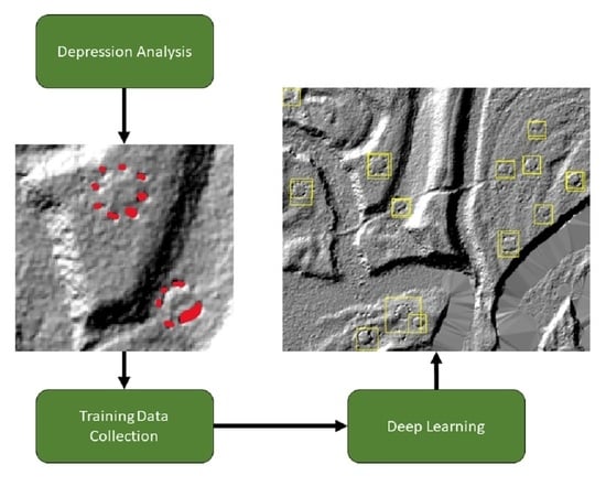
A Solution to Training Data Issues: Hydrological Depression Algorithms

Depression algorithms have been utilized by archaeologists for a range of purposes from crater detection to mound and shipwreck identification [27,40,41,42,43]. In the past several years, researchers developed a depression algorithm designed for sinkhole detection that works using a contour-tree procedure [44] wherein a computer looks for changes in elevation contours to locate high and low points in a region. Specifically, the algorithm locates low-lying points and searches for subsequently higher elevations surrounding that point to identify sinks (or depressions) on a landscape [44]. Wu et al. [44] demonstrated that using a contour tree process results in an exponentially faster processing time than previous methods, such as the stochastic depression algorithm [45], which has been used by archaeologists (e.g., ref [19]). Recently, researchers used this contour-tree method to automatically detect shipwrecks in bathymetric datasets in North America [41], thereby demonstrating its utility for cultural heritage research.

3. Materials and Methods

Extensive historical production of charcoal leaves discernable topographic scars on the present landscape. The availability of LiDAR data from Lantmäteriet, a Swedish governmental agency, permits a detailed analysis of the extent of centuries of charcoal production activities throughout forested regions of Sweden. Advances in machine learning and automation, likewise, offer great potential to record these deposits with speed and precision throughout large areas. Although tens-of-thousands of charcoal piles are recorded in Sweden’s National Heritage databases, local variations are not well documented. Therefore, we assessed the ability for a sinkhole detection algorithm to locate resmila charcoal piles because this method does not require training data. Then, we used the results of this analysis to compile training data to train a RetinaNet DL model.

3.1. Depression Algorithm

We used the Contour-Tree Depression Tool developed by Wu et al. [44,46] to detect small-circular depressions associated with charcoal production (see Figure 1c). The tool runs in ArcMap. We generated a Digital Elevation Model (DEM) with 1 m spatial resolution from LAS point data provided by Lantmäteriet with between 1 and 2 return points per square meter and used this DEM as input for the depression analysis. We ran the algorithm using a buffer size of 2 m and a minimum size of 5 m. Once the algorithm ran, we calculated the circularity of each detected depression using the equation:

$$C=\frac{4\pi A}{P^2}$$

(1)

where C = circularity, A = area, and P = perimeter. Area and perimeter were calculated using the Calculate Geometry tool, and circularity was calculated using the field calculator tool in ArcGIS 10.8 [47]. Next, we calculated topographic roughness, which characterizes the topography of a given region, using the formula developed by Riley et al. [48]:

$$TR=\frac{Mean-Minimum}{Maximum-Minimum}$$

(2)

where the neighborhood mean, minimum, and maximum values of the DEM are used to calculate roughness. Neighborhood values were generated using the focal statistics tool in ArcGIS 10.8 [47]. The values from the resulting raster were extracted for each location identified by the depression algorithm using zonal statistics. Finally, we reduced the results of the contour-tree depression analysis using circularity (>0.5) and topographic roughness values (mean > 60, range > 5).

3.2. Deep Learning with RetinaNet

RetinaNet architecture was predicated on a Feature Pyramid Network (FPN) and Focal Loss. FPNs are an architecture for processing data wherein low resolution data are combined with high-resolution data through a process of downsampling and upsampling (see Figure 4; ref [38]). Focal Loss alleviates the problem of having an overwhelming number of candidate objects, which often results in decreased accuracy for single-stage detectors [37].

RetinaNet operates on four main components (Figure 4): a bottom-up pathway, a top-down pathway, a classification subnetwork, and a regression subnetwork. The bottom-up pathway calculates a set of features at specific locations (or feature maps) at multiple scales. The top-down pathway up-samples the coarser feature maps and merges them with the bottom-up feature maps of the same size. Next, the classification subnetwork calculates the probability of an object being present at a given location and belonging to a specific class (defined by training data). The regression subnetwork then creates a labeled object from that classification (For more information about RetinaNet, see Lin et al. [37,38]. More information on RetinaNet in ArcGIS Pro can also be found at https://developers.arcgis.com/python/guide/how-retinanet-works/accessed on 25 October 2019).

3.3. Implementing RetinaNet CNN in ArcGIS Pro

We created a composite raster consisting of a DEM, hillshade, and slope map for the study region (following ref [31]) to create training data for the RetinaNet Model. ArcGIS Pro requires a multiband raster for deep learning applications. Using the pit features detected from the depression analysis, we labeled charcoal pit locations using the Label Training Data for Deep Learning Analysis tool in ArcGIS Pro 2.6 [39]. In total, we labeled 155 charcoal piles.

The number of documented charcoal piles was still somewhat limited, so we used augmentation procedures to increase our sample size. We augmented the training data using 90° rotations, thereby creating synthetic data that increased our sample sizes by a factor of 4. Using augmentation, we created a total of 940 images of charcoal piles with a size of 200 × 200 pixels using the Export Training Data for Deep Learning tool in ArcGIS Pro [39]. Other image dimensions were tested (248 × 248, 100 × 100) but resulted in lower model performance.

Next, we trained four different RetinaNet models using a ResNet 34, ResNet 50, ResNet 101, and ResNet 151 backbone model (Figure 5) with a batch size of 4, optimized learning rates, 10% validation, and 50 epochs. We also set the training to use an unfrozen model and to stop training if improvements stopped. We chose a batch size of 4 to ensure that the process could be implemented on computers without CUDA GPU processors, which are quite expensive and can limit the usability of this method. Models were trained on multiple computers, including a personal laptop with 8 GB of RAM, an Intel Core i7-4510U CPU @ 2.0 GHz with two cores and four logical processors to ensure our method can be utilized by researchers with a range of computational resource availability. ResNet (Residual Network, He et al. 2017) is a transfer learning architecture that is trained on the ImageNet dataset (consisting of over 1 million images) and contains different numbers of layers and helps to improve both the speed and accuracy of the model training process. Here, we used ResNet with 34, 50, 101, and 152 layers. We set up the training procedure to run each model 50 times (50 epochs) and to stop training when the model was no longer improving, in order to save time and processing power. To evaluate overfitting issues with the model, we withheld 10% of the training data for validation.

Once the model was trained, we evaluated its performance by detecting objects within the boundaries of two LiDAR tiles from Jönköping County, Sweden, via the Detect Objects Using Deep Learning tool in ArcGIS Pro [39]. Newly detected charcoal piles were added to the training dataset, and we trained another RetinaNet Model using the best performing backbone architecture from the initial set of tests. Due to the ongoing COVID-19 pandemic, ground evaluation has not yet been conducted, but will constitute the focus of future research. For the purpose of this study, we are still able to demonstrate the utility of these techniques for expanding archaeological investigations on charcoal production in Northern Europe.

4. Results

4.1. Depression Analysis Results

The Wu et al. [44] contour tree algorithm detected 768 possible depressions related to charcoal production. We checked each of these identifications manually by assessing morphology, location, and conformity with known examples of resmila. This manual evaluation led to the confirmation of 243 depressions related to charcoal piles within the study area and 38 possibly related to charcoal production (accuracy = 33.3%). Future ground testing will confirm or reject these possible charcoal production locations. Among the 243 identified depressions were 180 charcoal pit sites. We used a selection of 155 of these detections to train a series of RetinaNet models (see Section 3.2). We excluded 25 depressions and retained them for validation of our RetinaNet models.

4.2. RetinaNet Results

Using a selection of the best-preserved charcoal pit features detected using the depression algorithm, we trained four different RetinaNet models using different transfer learning architectures. The results of these models are listed in

Table 1. Results of RetinaNet models trained using samples collected from depression analysis.

Transfer Learning Architecture	Learning Rate	Accuracy	Training Loss	Validation Loss
ResNet34	8.3 × 10−5	59%	1.7295	1.9112
ResNet50	6.3 × 10−6	63%	1.8222	1.2973
ResNet101	0.0001	55%	0.8254	1.0824
ResNet152	4.8 × 10−5	61%	0.6316	0.8489

. Using these models, we ran the ResNet50 and ResNet152 models on the same test area as the depression analysis to further evaluate each model’s performance (Figure 6).

When comparing the ResNet50 and ResNet152 models, both detected a similar number of features with minimal false positives (Figure 7). The model trained on ResNet152 identified three more training data locations than the ResNet50 model and both had similar numbers of false negatives. The ResNet50 model had fewer false positives than the ResNet152 model (n = 16 and n = 29, respectively).

Following this analysis, we incorporated newly detected charcoal piles from the initial RetinaNet models as training data to improve the model trained on ResNet50. The new model was trained using a larger batch size of 8 because smaller batch sizes resulted in lower accuracy (<60%). This new model achieved a slightly higher accuracy of 64.15% and lower loss values for both training and validation data (1.12 and 1.05, respectively), indicating greater utility across larger areas.

5. Discussion

We demonstrated how hydrological depression algorithms can be used to collect preliminary training data for DL models. The depression analysis resulted in many false positives, however, which require expert analysts to manually evaluate before choosing appropriate training datasets. Nevertheless, this procedure allowed us to generate more than 150 examples of charcoal piles within our study area which trained our initial DL model. This iterative detection process can aid in the identification of archaeological features at landscape scales with high degrees of accuracy and survey coverage, particularly in areas where available archaeological data are initially limited, or where knowledge about particular kinds of features are less well-established. In this study, our false positives decreased at each stage, from ~67% with hydrological depression methods to less than 14% with our first ResNet50 model. False positives also appeared to decrease with each iteration but were present in all methods deployed (see Figure 7). Furthermore, by consistently reapplying DL models with new training data identified during previous model runs, we showed how automated detection can be utilized in an iterative manner to improve archaeological recording efforts (see Figure 8). This can greatly increase the utility of advanced automated methods of remote sensing analysis among archaeologists working in regions with limited landscape scale archaeological records.

Despite expanding the utility of automated analysis methods to case studies with limited training data availability, one key limitation of many applications of DL is computational requirements. Most applications of DL for archaeological prospection utilize dual-stage model architectures (e.g., R-CNN). While these models result in high accuracy in many cases, they are also computationally expensive and require high-performance GPU processors to run effectively, placing their use outside of the realm of possibility for many researchers. Here, we made use of a single-stage DL model (RetinaNet) and demonstrated how these models can be trained without CUDA GPU processors. This opens the possibilities of DL applications to a greater number of archaeologists. In the future, we plan to expand our application of the DL models generated here to investigate the spatial extent and total quantity of resmila charcoal pit features across Sweden’s forested landscape.

With continued analyses, the remains of charcoal piles can be placed in a comprehensive cultural–historical context with the foundry Järnbruket Hörle bruk, which is located nearby our study area. This means that there is likely to be a plethora of historical records that can be processed in order to reach conclusions on organization, as well as economic and social aspects of charcoal production. Moreover, spatial analyses of the locations of these charcoal piles remain an unexplored research topic, and having a more comprehensive record of the geographic distribution of charcoal piles could be achieved using the data generated from automated LiDAR analyses (e.g., [42,43,49,50]). Where clusters of charcoal pits remain, future work can also investigate if other constructions related to charcoal production, such as huts and storage piles, are located nearby, and attempts to automate the detection of these features can form future research objectives. Finally, with a systematic record of charcoal production for the area, future research can focus on paleoecological analysis based on pollen records to analyse the intensity of the production in a certain area based on ash deposits. Such work can also provide a better understanding of the development of vegetation on the landscape over time.

The identification and localization of these sites—especially if many prove to predate 1850—would result in them being registered as National Heritage Sites by the Swedish National Heritage Board, which would then protect them under Swedish law. Fieldwork conducted by one of the authors (JL) suggests that many of these remains would be overlooked by non-archaeologists because of their subtle appearance in a constantly changing landscape. Thus, the destructive nature of the forest industry may lead to many charcoal production features becoming damaged or completely unidentifiable in the future. The sheer number of these remains, along with the fact that they are overlooked, places them at risk of destruction. We hope that our methods for quickly identifying these structures in LiDAR assist in increasing attention towards these features and lead to many more charcoal piles being registered in archaeological site databases for future research.

6. Conclusions

This case study demonstrates the utility of single-stage RetinaNet DL models for identifying charcoal pit features in the forested regions of Sweden. Using a topographic depression analysis procedure, we collected the necessary training data to implement a DL model that successfully detects these charcoal features, demonstrating the power of an iterative approach to site prospection making use of multiple techniques. The ability to train single-stage DL models for archaeological site prospection will likely open the door for many more researchers to implement these methods because of their lower computational requirements when compared to most dual-stage methods commonly used within archaeology (e.g., R-CNN, Faster R-CNN, Mask R-CNN, etc.). Within Northern European and North American archaeology, generally, this research shows the potential for analyzing available LiDAR datasets in a systematic way to expedite cultural heritage monitoring and survey efforts, especially in the study of RCHs and other charcoal production methods. Furthermore, such techniques make it possible to examine more closely the history of anthropogenic landscape modifications in northern Europe and compare resource extraction between different areas.

References

1. Ågren, M. Iron-Making Societies: Early Industrial Development in Sweden and Russia, 1600–1900; Berghahn Books: Brooklyn, NY, USA, 1998. [Google Scholar]
2. Petterssen, J.E. (Ed.) Svenskt Järn Under 2500 år: Från Gruvpigor och Smeddrängar till Operatörer; Bokbörsen AB: Stockholm, Sweden, 1997. [Google Scholar]
3. Svensson, E. Människor i Utmark. [Lund Studies in Medieval Archaeology 21]; Lund University: Lund, Sweden, 1998. [Google Scholar]
4. Deforce, K.; Groenewoudt, B.; Haneca, K. 2500 Years of Charcoal Production in the Low Countries: The Chronology and Typology of Charcoal Kilns and Their Relation with Early Iron Production. Quat. Int. 2021, 593–594, 295–305. [Google Scholar] [CrossRef]
5. Hennius, A. Spår Av Kolning: Arkeologiskt Kunskapsunderlag Och Forskningsöversikt; Riksantikvarieämbetet: Stockholm, Sweden, 2019. [Google Scholar]
6. Arpi, G. The Supply with Charcoal of the Swedish Iron Industry from 1830 to 1950. Geogr. Ann. 1953, 35, 11–27. [Google Scholar]
7. Jernkontoret Svenska Järn- och Stålindustrins Historia. Available online: https://www.jernkontoret.se/sv/stalindustrin/stalindustrins-historia/ (accessed on 3 August 2021).
8. Anglert, M.; Lagerås, P. (Eds.) Människorna Och Skogen: Arkeologiska Platser i Örkelljungatrakten; Riksantikvarieämbetet: Stockholm, Sweden, 2009. [Google Scholar]
9. Stereńczak, K.; Zapłata, R.; Wójcik, J.; Kraszewski, B.; Mielcarek, M.; Mitelsztedt, K.; Białczak, M.; Krok, G.; Kuberski, Ł.; Markiewicz, A.; et al. ALS-Based Detection of Past Human Activities in the Białowieża Forest—New Evidence of Unknown Remains of Past Agricultural Systems. Remote Sens. 2020, 12, 2657. [Google Scholar] [CrossRef]
10. Zapłata, R.; Bakuła, K.; Ostrowski, W. Transformation Methods and ALS-Data Visualization in the Studies of Historical Charcoal Piles. In Proceedings of the International Multidisciplinary Scientific Conferences on Social Sciences and Arts SGEM2014, Albena, Bulgaria, 2–7 September 2014; pp. 417–424. [Google Scholar]
11. Wilmshurst, J.M.; Hunt, T.L.; Lipo, C.P.; Anderson, A.J. High-Precision Radiocarbon Dating Shows Recent and Rapid Initial Human Colonization of East Polynesia. Proc. Natl. Acad. Sci. USA 2011, 108, 1815–1820. [Google Scholar] [CrossRef] [PubMed] [Green Version]
12. Bonhage, A.; Eltaher, M.; Raab, T.; Breuß, M.; Raab, A.; Schneider, A. A Modified Mask Region-Based Convolutional Neural Network Approach for the Automated Detection of Archaeological Sites on High-Resolution Light Detection and Ranging-Derived Digital Elevation Models in the North German Lowland. Archaeol. Prospect. 2021, 28, 177–186. [Google Scholar] [CrossRef]
13. Carter, V.A.; Brunelle, A.; Power, M.J.; DeRose, R.J.; Bekker, M.F.; Hart, I.; Brewer, S.; Spangler, J.; Robinson, E.; Abbott, M.; et al. Legacies of Indigenous Land Use Shaped Past Wildfire Regimes in the Basin-Plateau Region, USA. Commun. Earth Environ. 2021, 2, 72. [Google Scholar] [CrossRef]
14. Schneider, A.; Takla, M.; Nicolay, A.; Raab, A.; Raab, T. A Template-Matching Approach Combining Morphometric Variables for Automated Mapping of Charcoal Kiln Sites: Automated Mapping of Charcoal Kiln Sites. Archaeol. Prospect. 2015, 22, 45–62. [Google Scholar] [CrossRef]
15. Raab, A.; Takla, M.; Raab, T.; Nicolay, A.; Schneider, A.; Rösler, H.; Heußner, K.-U.; Bönisch, E. Pre-Industrial Charcoal Production in Lower Lusatia (Brandenburg, Germany): Detection and Evaluation of a Large Charcoal-Burning Field by Combining Archaeological Studies, GIS-Based Analyses of Shaded-Relief Maps and Dendrochronological Age Determination. Quat. Int. 2015, 367, 111–122. [Google Scholar] [CrossRef]
16. Hirsch, F.; Raab, T.; Ouimet, W.; Dethier, D.; Schneider, A.; Raab, A. Soils on Historic Charcoal Hearths: Terminology and Chemical Properties. Soil Sci. Soc. Am. J. 2017, 81, 1427–1435. [Google Scholar] [CrossRef] [Green Version]
17. Donovan, S.; Ignatiadis, M.; Ouimet, W.; Dethier, D.; Hren, M. Gradients of Geochemical Change in Relic Charcoal Hearth Soils, Northwestern Connecticut, USA. Catena 2021, 197, 104991. [Google Scholar] [CrossRef]
18. Rutkiewicz, P.; Malik, I.; Wistuba, M.; Osika, A. High Concentration of Charcoal Hearth Remains as Legacy of Historical Ferrous Metallurgy in Southern Poland. Quat. Int. 2019, 512, 133–143. [Google Scholar] [CrossRef]
19. Boheman, E. (Ed.) Svenska Turistföreningens Årsskrift 1921; Wahlström & Widstrand: Stockholm, Sweden, 1921. [Google Scholar]
20. Davis, D.S. Object-Based Image Analysis: A Review of Developments and Future Directions of Automated Feature Detection in Landscape Archaeology. Archaeol. Prospect. 2019, 26, 155–163. [Google Scholar] [CrossRef]
21. Magnini, L.; Bettineschi, C. Theory and Practice for an Object-Based Approach in Archaeological Remote Sensing. J. Archaeol. Sci. 2019, 107, 10–22. [Google Scholar] [CrossRef]
22. Traviglia, A.; Torsello, A. Landscape Pattern Detection in Archaeological Remote Sensing. Geosciences 2017, 7, 128. [Google Scholar] [CrossRef] [Green Version]
23. Agapiou, A. Optimal Spatial Resolution for the Detection and Discrimination of Archaeological Proxies in Areas with Spectral Heterogeneity. Remote Sens. 2020, 12, 136. [Google Scholar] [CrossRef] [Green Version]
24. Caspari, G.; Crespo, P. Convolutional Neural Networks for Archaeological Site Detection—Finding “Princely” Tombs. J. Archaeol. Sci. 2019, 110, 104998. [Google Scholar] [CrossRef]
25. Cerrillo-Cuenca, E. An Approach to the Automatic Surveying of Prehistoric Barrows through LiDAR. Quat. Int. 2017, 435, 135–145. [Google Scholar] [CrossRef]
26. Davis, D.S.; Lipo, C.P.; Sanger, M.C. A Comparison of Automated Object Extraction Methods for Mound and Shell-Ring Identification in Coastal South Carolina. J. Archaeol. Sci. Rep. 2019, 23, 166–177. [Google Scholar] [CrossRef]
27. Freeland, T.; Heung, B.; Burley, D.V.; Clark, G.; Knudby, A. Automated Feature Extraction for Prospection and Analysis of Monumental Earthworks from Aerial LiDAR in the Kingdom of Tonga. J. Archaeol. Sci. 2016, 69, 64–74. [Google Scholar] [CrossRef]
28. Verschoof-van der Vaart, W.B.; Landauer, J. Using CarcassonNet to Automatically Detect and Trace Hollow Roads in LiDAR Data from the Netherlands. J. Cult. Herit. 2020, 47, 143–154. [Google Scholar] [CrossRef]
29. Verschoof-van der Vaart, W.B.; Lambers, K. Learning to Look at LiDAR: The Use of R-CNN in the Automated Detection of Archaeological Objects in LiDAR Data from the Netherlands. J. Comput. Appl. Archaeol. 2019, 2, 31–40. [Google Scholar] [CrossRef] [Green Version]
30. Trier, Ø.D.; Cowley, D.C.; Waldeland, A.U. Using Deep Neural Networks on Airborne Laser Scanning Data: Results from a Case Study of Semi-Automatic Mapping of Archaeological Topography on Arran, Scotland. Archaeol. Prospect. 2019, 26, 165–175. [Google Scholar] [CrossRef]
31. Davis, D.S.; Caspari, G.; Lipo, C.P.; Sanger, M.C. Deep Learning Reveals Extent of Archaic Native American Shell-Ring Building Practices. J. Archaeol. Sci. 2021, 132, 105433. [Google Scholar] [CrossRef]
32. Lambers, K.; Verschoof-van der Vaart, W.; Bourgeois, Q. Integrating Remote Sensing, Machine Learning, and Citizen Science in Dutch Archaeological Prospection. Remote Sens. 2019, 11, 794. [Google Scholar] [CrossRef] [Green Version]
33. Somrak, M.; Džeroski, S.; Kokalj, Ž. Learning to Classify Structures in ALS-Derived Visualizations of Ancient Maya Settlements with CNN. Remote Sens. 2020, 12, 2215. [Google Scholar] [CrossRef]
34. Davis, D.S. Geographic Disparity in Machine Intelligence Approaches for Archaeological Remote Sensing Research. Remote Sens. 2020, 12, 921. [Google Scholar] [CrossRef] [Green Version]
35. Tan, C.; Sun, F.; Kong, T.; Zhang, W.; Yang, C.; Liu, C. A Survey on Deep Transfer Learning. In Artificial Neural Networks and Machine Learning, Proceedings of the International Conference on Artificial Neural Networks (ICANN 2018), Rhodes, Greece, 4–7 October 2018; Springer: Cham, Switzerland, 2018; pp. 270–279. [Google Scholar]
36. Trier, Ø.D.; Reksten, J.H.; Løseth, K. Automated Mapping of Cultural Heritage in Norway from Airborne Lidar Data Using Faster R-CNN. Int. J. Appl. Earth Obs. Geoinf. 2021, 95, 102241. [Google Scholar] [CrossRef]
37. Lin, T.-Y.; Goyal, P.; Girshick, R.; He, K.; Dollár, P. Focal Loss for Dense Object Detection. In Proceedings of the IEEE International Conference on Computer Vision, Venice, Italy, 22–29 October 2017; pp. 2980–2988. [Google Scholar]
38. Lin, T.-Y.; Dollár, P.; Girshick, R.; He, K.; Hariharan, B.; Belongie, S. Feature Pyramid Networks for Object Detection. In Proceedings of the IEEE Conference on Computer Vision and Pattern Recognition, Venice, Italy, 22–29 October 2017; pp. 2117–2125. [Google Scholar]
39. ESRI. ArcGIS Pro; Environmental Systems Research Institute, Inc.: Redlands, CA, USA, 2020. [Google Scholar]
40. Davis, D.S.; Sanger, M.C.; Lipo, C.P. Automated Mound Detection Using Lidar and Object-Based Image Analysis in Beaufort County, South Carolina. Southeast. Archaeol. 2019, 38, 23–37. [Google Scholar] [CrossRef]
41. Davis, D.S.; Buffa, D.C.; Wrobleski, A.C. Assessing the Utility of Open-Access Bathymetric Data for Shipwreck Detection in the United States. Heritage 2020, 3, 364–383. [Google Scholar] [CrossRef]
42. Dolejš, M.; Pacina, J.; Veselý, M.; Brétt, D. Aerial Bombing Crater Identification: Exploitation of Precise Digital Terrain Models. ISPRS Int. J. Geo-Inf. 2020, 9, 713. [Google Scholar] [CrossRef]
43. Rom, J.; Haas, F.; Stark, M.; Dremel, F.; Becht, M.; Kopetzky, K.; Schwall, C.; Wimmer, M.; Pfeifer, N.; Mardini, M.; et al. Between Land and Sea: An Airborne LiDAR Field Survey to Detect Ancient Sites in the Chekka Region/Lebanon Using Spatial Analyses. Open Archaeol. 2020, 6, 248–268. [Google Scholar] [CrossRef]
44. Wu, Q.; Liu, H.; Wang, S.; Yu, B.; Beck, R.; Hinkel, K. A Localized Contour Tree Method for Deriving Geometric and Topological Properties of Complex Surface Depressions Based on High-Resolution Topographical Data. Int. J. Geogr. Inf. Sci. 2015, 29, 2041–2060. [Google Scholar] [CrossRef]
45. Lindsay, J.B.; Creed, I.F. Distinguishing Actual and Artefact Depressions in Digital Elevation Data. Comput. Geosci. 2006, 32, 1192–1204. [Google Scholar] [CrossRef]
46. Wu, Q.; Deng, C.; Chen, Z. Automated Delineation of Karst Sinkholes from LiDAR-Derived Digital Elevation Models. Geomorphology 2016, 266, 1–10. [Google Scholar] [CrossRef]
47. ESRI. ArcGIS; Environmental Systems Research Institute, Inc.: Redlands, CA, USA, 2020. [Google Scholar]
48. Riley, S.J.; DeGloria, S.D.; Elliot, R. Index That Quantifies Topographic Heterogeneity. Intermt. J. Sci. 1999, 5, 23–27. [Google Scholar]
49. Davis, D.S.; DiNapoli, R.J.; Sanger, M.C.; Lipo, C.P. The Integration of Lidar and Legacy Datasets Provides Improved Explanations for the Spatial Patterning of Shell Rings in the American Southeast. Adv. Archaeol. Pract. 2020, 8, 361–375. [Google Scholar] [CrossRef]
50. Cerrillo-Cuenca, E.; Bueno-Ramírez, P. Counting with the Invisible Record? The Role of LiDAR in the Interpretation of Megalithic Landscapes in South-western Iberia (Extremadura, Alentejo and Beira Baixa). Archaeol. Prospect. 2019, 26, 251–264. [Google Scholar] [CrossRef]
Figure 1. (A). Historical image of resmila in use for coal production (credit: ref [19]). (B). Schematic drawing of resmila charcoal piles (credit: ref [5]). (C). Two examples of resmila in a LiDAR-derived hillshade map (indicated by yellow arrows). These features range in size (10–20 m) in terms of diameter.
Remotesensing 13 03680 g001
Figure 2. Workflow of automated analysis of LiDAR for the detection of charcoal piles.
Remotesensing 13 03680 g002
Figure 3. Map of the study region. The black box shows the geographic extent of the LiDAR analyzed in this article.
Remotesensing 13 03680 g003
Figure 4. RetinaNet model architecture. (A,B) represent the FPN, with (A) consisting of a backbone model (in our case ResNet 50) that uses a bottom-up pathway to create feature maps at different scales from increasingly lower resolution data. The thicker the black outline on the boxes, the stronger the prediction. (B) is the top-down pathway, where feature maps are created from low-resolution data and enhanced with higher-resolution feature data from lateral connections (arrows) with the bottom-up pathway (A). Predictions made in (C) are divided into two components: Class and box subnets (D). Class subnets determine the probability of a given area containing an object. Box subnets label objects within class subnets.
Remotesensing 13 03680 g004
Figure 5. ArcGIS tool settings for deep learning implementation. For the Training Deep Learning Model Tool, the ResNet backbone was changed from ResNet 34, ResNet50, ResNet101, and ResNet152 for each of the models reported below.
Remotesensing 13 03680 g005aRemotesensing 13 03680 g005b
Figure 6. Loss values for the RetinaNet model using the (A) ResNet50 backbone and (B) ResNet152 backbone.
Remotesensing 13 03680 g006
Figure 7. Comparison of detections of charcoal piles by the depression analysis and the two best performing RetinaNet models trained on ResNet50 and ResNet152. Black arrows show locations of charcoal pit features that were missed by all of the automation methods. Hillshade basemap created from Laserdata NH GSD- © Lantmäteriet (2012).
Remotesensing 13 03680 g007
Figure 8. Total distribution of charcoal piles identified by the methods used in this study. Approximately 180 piles were detected between hydrological depression and RetinaNet analyses.
Remotesensing 13 03680 g008