
Real-Time Automated Classification of Sky Conditions Using Deep Learning and Edge Computing

 ,
,  ,
,
Abstract
:
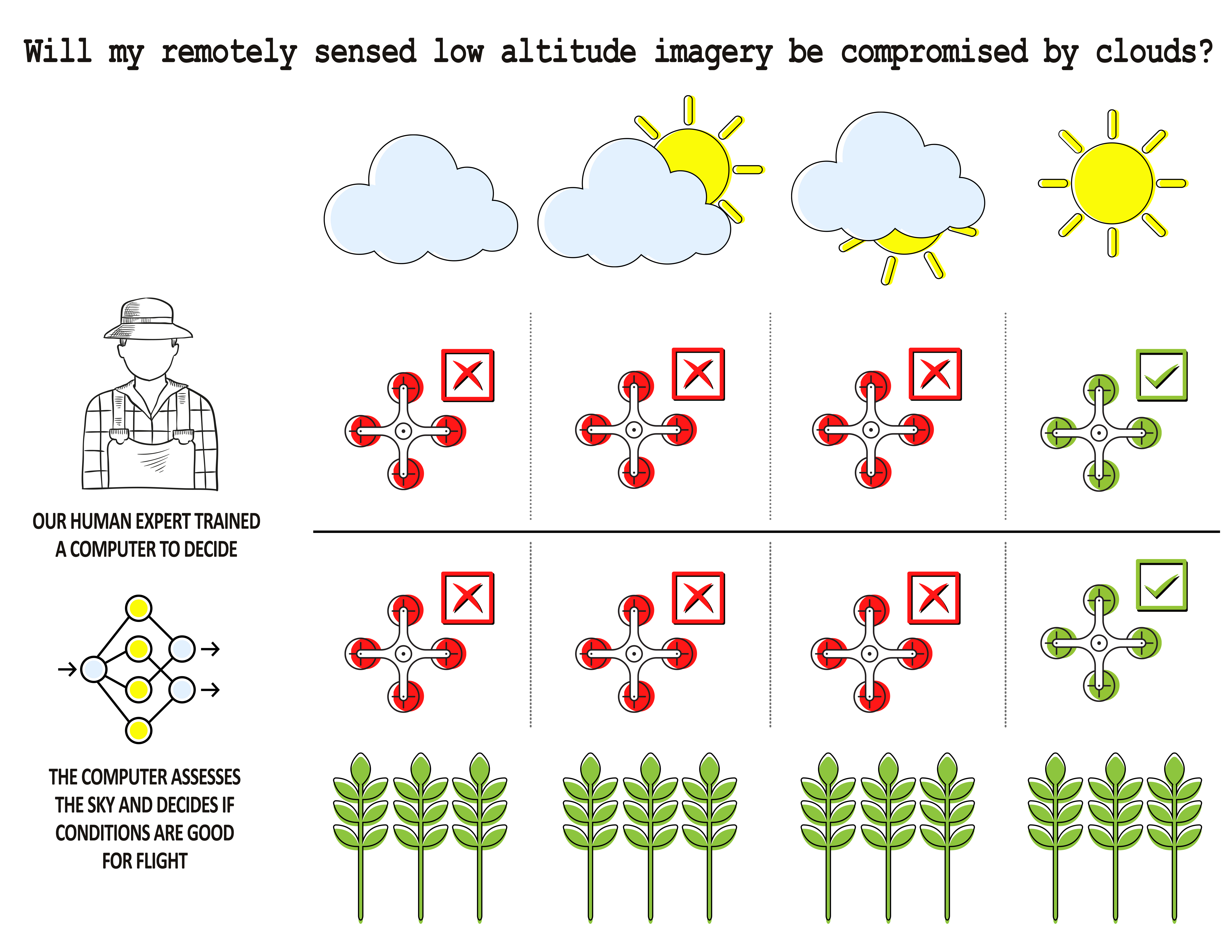
1. Introduction
2. Materials and Methods
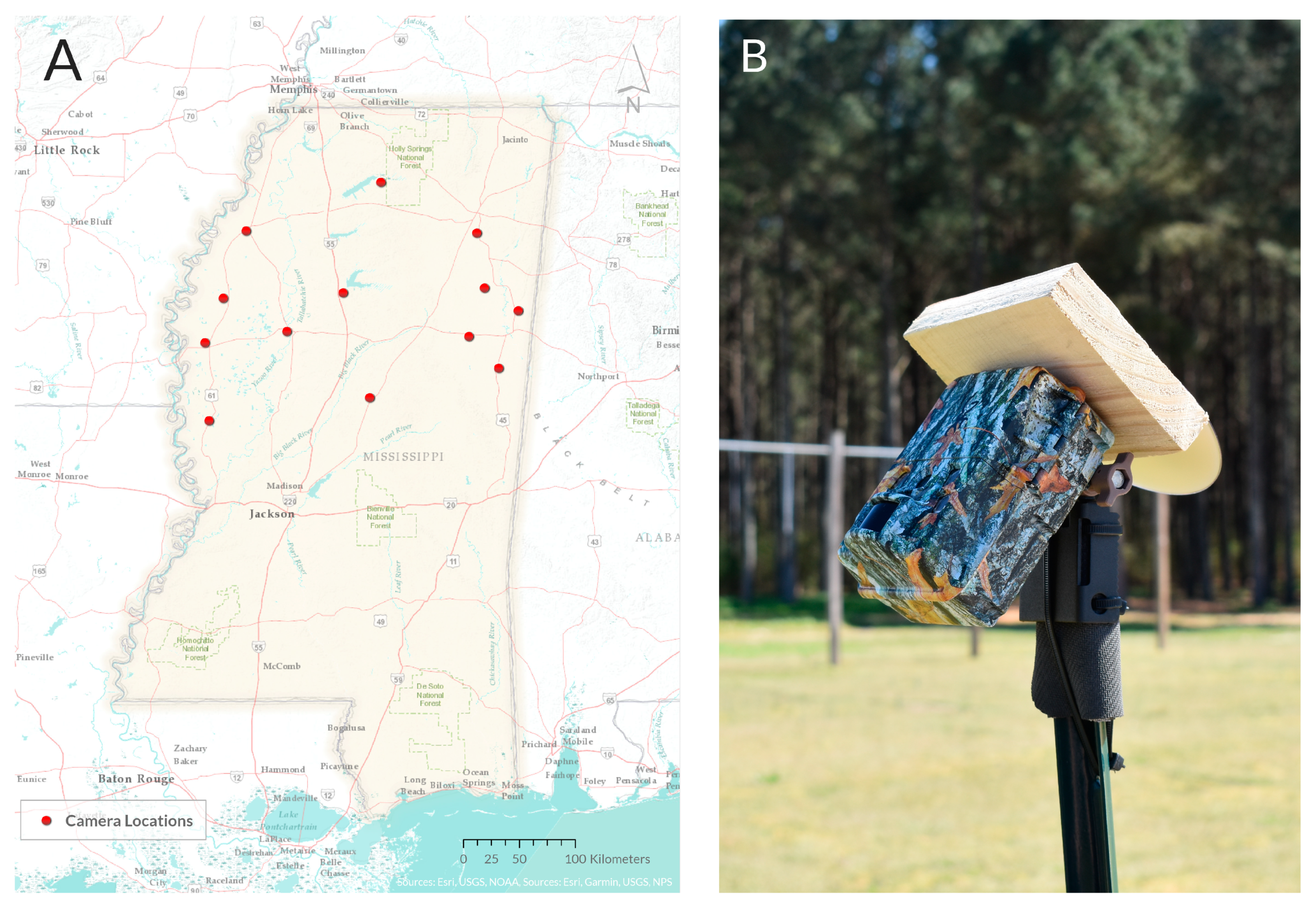
2.1. Data Collection
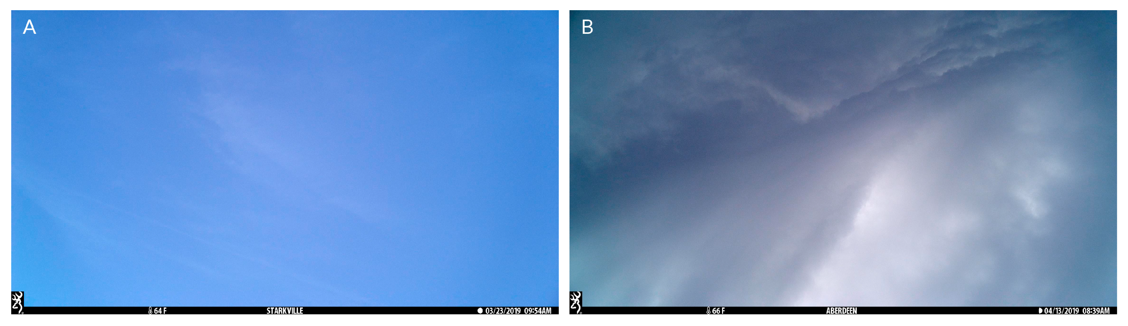
2.2. Data Labeling
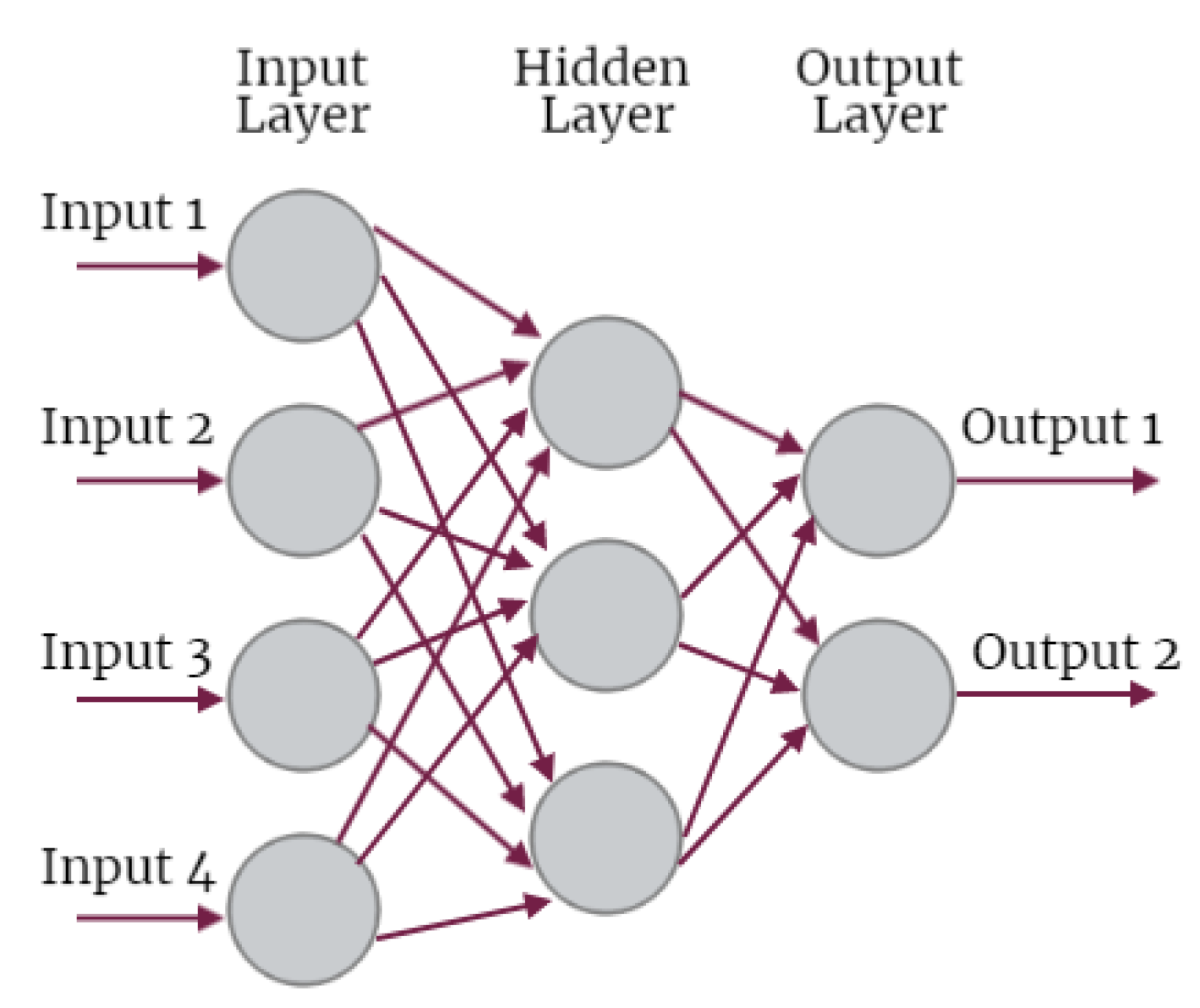
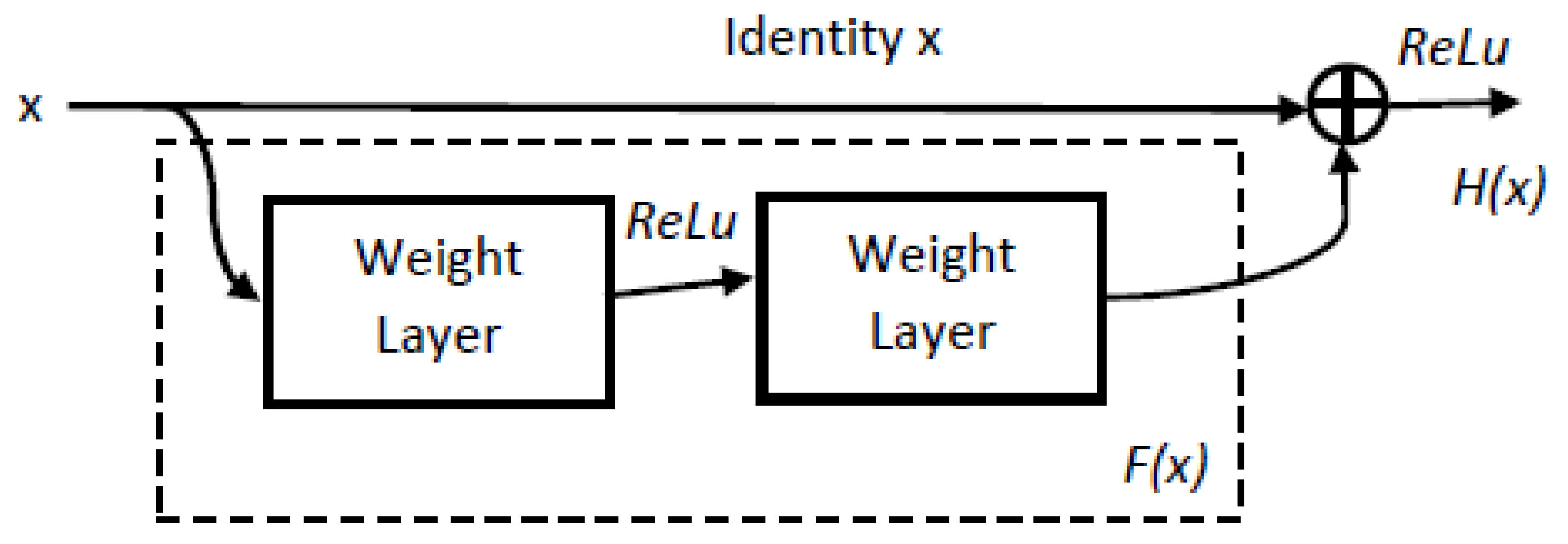
2.3. Deep Learning Networks
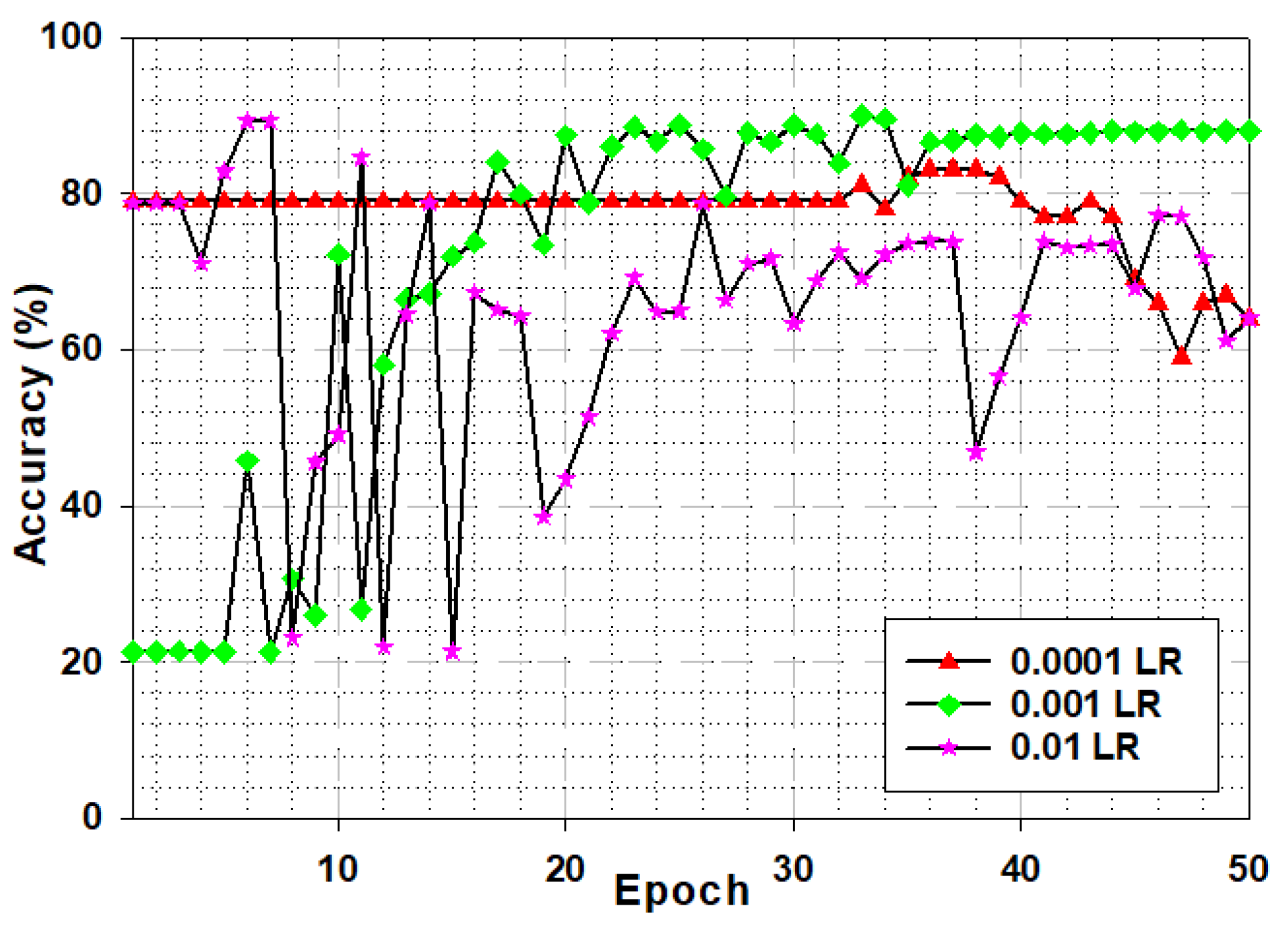
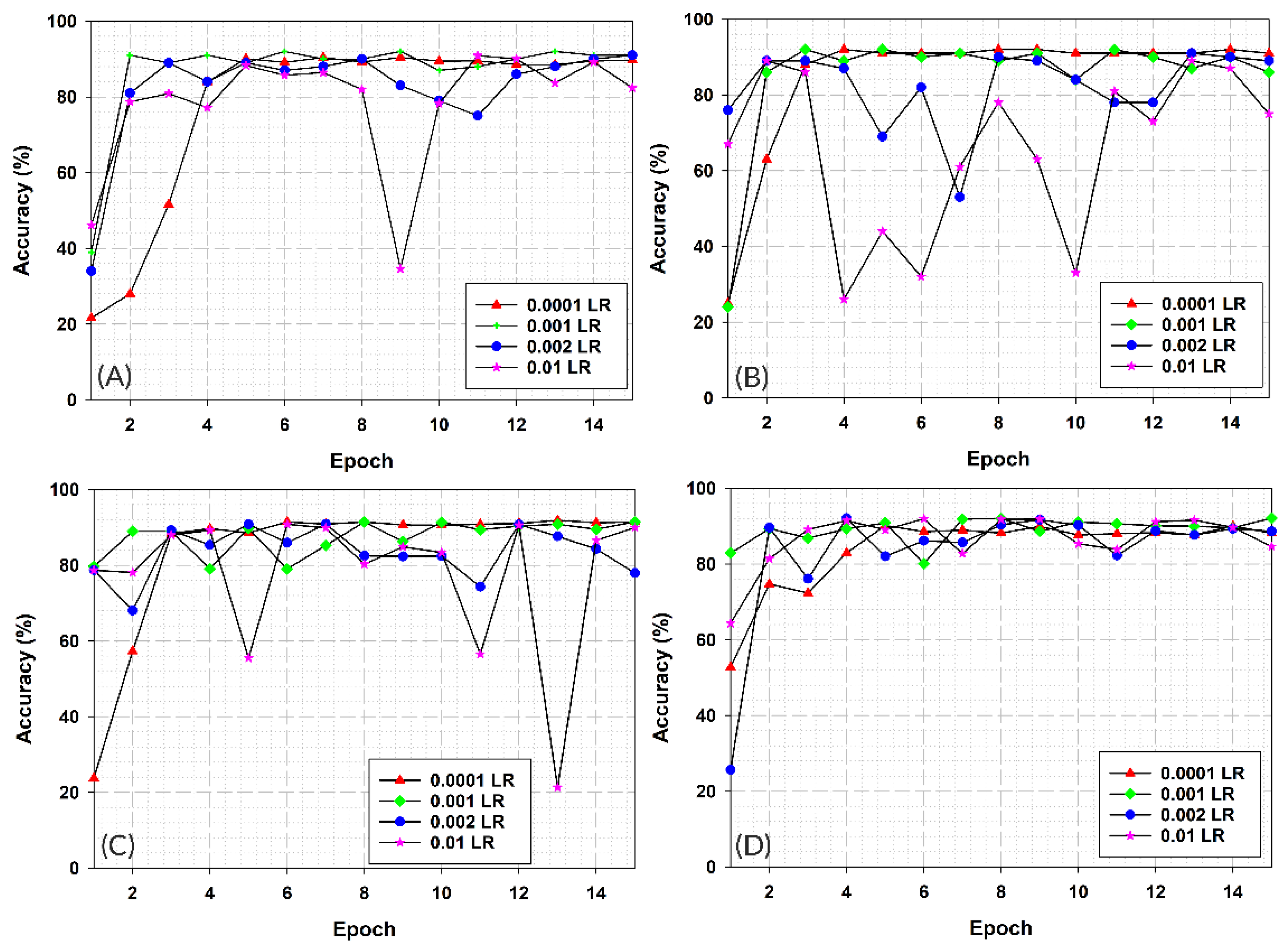
2.4. Network Training
2.5. Transition to Edge Computer Platform
2.6. Comparison to Human Model
3. Results
4. Discussion
5. Conclusions
Author Contributions
Funding
Institutional Review Board Statement
Informed Consent Statement
Data Availability Statement
Acknowledgments
Conflicts of Interest
References
- Thorp, K.; Tian, L. A Review on Remote Sensing of Weeds in Agriculture. Precis. Agric. 2004, 5, 477–508. [Google Scholar] [CrossRef]
- Dadhwal, V.; Ray, S. Crop Assessment Using Remote Sensing-Part II: Crop Condition and Yield Assessment. Indian J. Agric. Econ. 2000, 55, 55–67. [Google Scholar]
- Ozdogan, M.; Yang, Y.; Allez, G.; Cervantes, C. Remote Sensing of Irrigated Agriculture: Opportunities and Challenges. Remote Sens. 2010, 2, 2274–2304. [Google Scholar] [CrossRef] [Green Version]
- Kasampalis, D.A.; Alexandridis, T.K.; Deva, C.; Challinor, A.; Moshou, D.; Zalidis, G. Contribution of Remote Sensing on Crop Models: A Review. J. Imaging 2018, 4, 52. [Google Scholar] [CrossRef] [Green Version]
- Chauhan, S.; Darvishzadeh, R.; Boschetti, M.; Pepe, M.; Nelson, A. Remote Sensing-Based Crop Lodging Assessment: Current Status and Perspectives. ISPRS J. Photogramm. 2019, 151, 124–140. [Google Scholar] [CrossRef] [Green Version]
- Eberhardt, I.D.R.; Schultz, B.; Rizzi, R.; Sanches, I.D.; Formaggio, A.R.; Atzberger, C.; Mello, M.P.; Immitzer, M.; Trabaquini, K.; Foschiera, W. Cloud Cover Assessment for Operational Crop Monitoring Systems in Tropical Areas. Remote Sens. 2016, 8, 219. [Google Scholar] [CrossRef] [Green Version]
- Ju, J.; Roy, D.P. The Availability of Cloud-Free Landsat ETM+ Data over the Conterminous United States and Globally. Remote Sens. Environ. 2008, 112, 1196–1211. [Google Scholar] [CrossRef]
- Boursianis, A.D.; Papadopoulou, M.S.; Diamantoulakis, P.; Liopa-Tsakalidi, A.; Barouchas, P.; Salahas, G.; Karagiannidis, G.; Wan, S.; Goudos, S.K. Internet of Things (IoT) and Agricultural Unmanned Aerial Vehicles (UAVs) in Smart Farming: A Comprehensive Review. Internet Things 2020, 100187. [Google Scholar] [CrossRef]
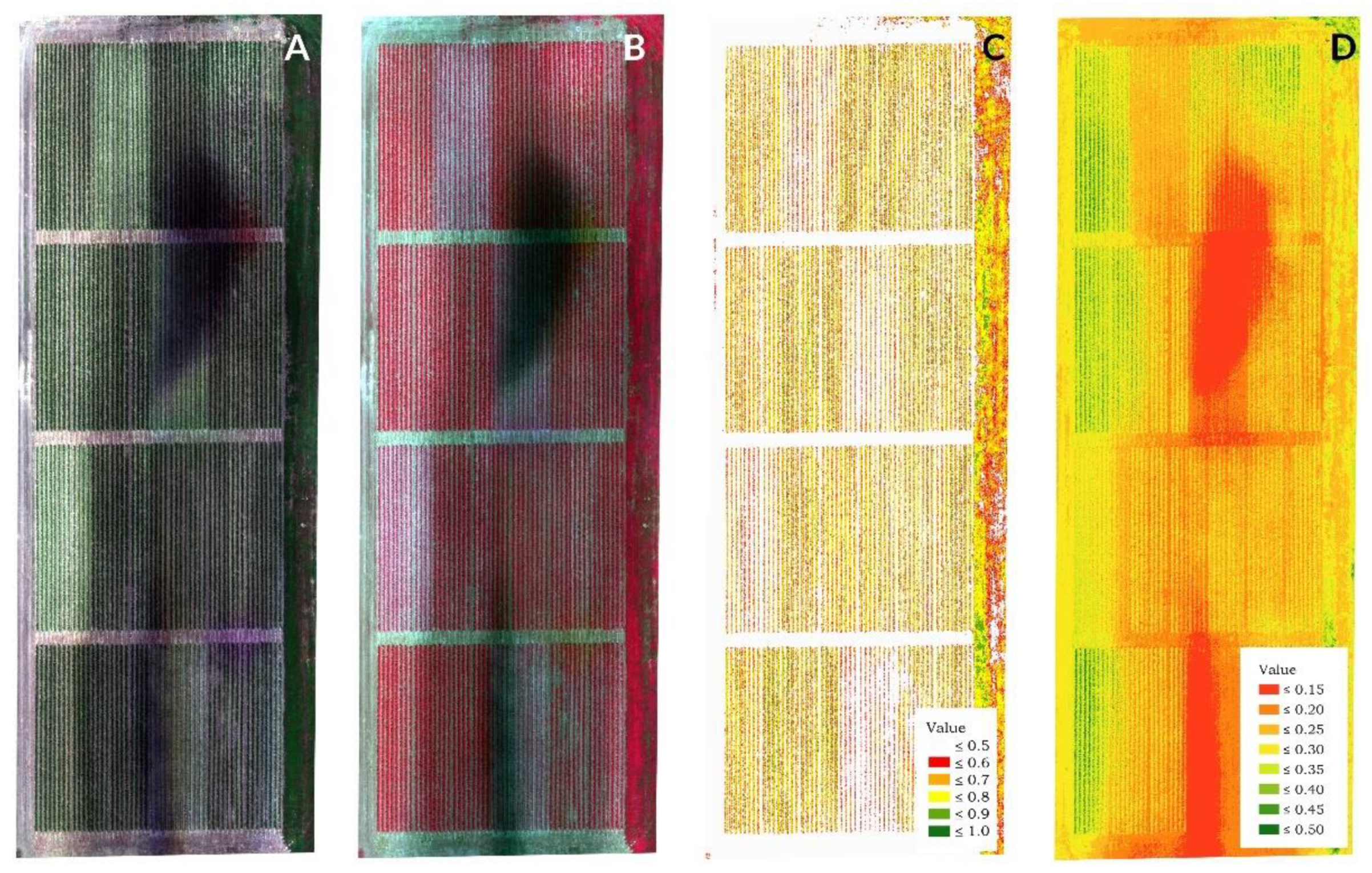
- Wierzbicki, D.; Fryskowska, A.; Kedzierski, M.; Wojtkowska, M.; Delis, P. Method of Radiometric Quality Assessment of NIR Images Acquired with a Custom Sensor Mounted on an Unmanned Aerial Vehicle. J. Appl. Remote Sens. 2018, 12, 015008. [Google Scholar] [CrossRef]
- Kedzierski, M.; Wierzbicki, D.; Sekrecka, A.; Fryskowska, A.; Walczykowski, P.; Siewert, J. Influence of Lower Atmosphere on the Radiometric Quality of Unmanned Aerial Vehicle Imagery. Remote Sens. 2019, 11, 1214. [Google Scholar] [CrossRef] [Green Version]
- Kaur, S. Handling Shadow Effects on Greenness Indices from Multispectral UAV Imagery. Master’s Thesis, School of Forest Science and Resource Management, Technical University of Munich, Munich, Germany, 2020. [Google Scholar]
- Zhang, L.; Sun, X.; Wu, T.; Zhang, H. An Analysis of Shadow Effects on Spectral Vegetation Indexes Using a Ground-Based Imaging Spectrometer. IEEE Geosci. Remote Sens. 2015, 12, 2188–2192. [Google Scholar] [CrossRef]
- Martín-Ortega, P.; García-Montero, L.G.; Sibelet, N. Temporal Patterns in Illumination Conditions and Its Effect on Vegetation Indices Using Landsat on Google Earth Engine. Remote Sens. 2020, 12, 211. [Google Scholar] [CrossRef] [Green Version]
- Kedzierski, M.; Wierzbicki, D. Radiometric Quality Assessment of Images Acquired by UAV’s in Various Lighting and Weather Conditions. Measurement 2015, 76, 156–169. [Google Scholar] [CrossRef]
- Han, Y.; Oruklu, E. Traffic Sign Recognition Based on the Nvidia Jetson Tx1 Embedded System Using Convolutional Neural Networks. In Proceedings of the 60th International Midwest Symposium on Circuits and Systems (MWSCAS), Medford, MA, USA, 6 August 2017; IEEE: Piscataway, NJ, USA, 2017; pp. 184–187. [Google Scholar]
- Lee, H.; Grosse, R.; Ranganath, R.; Ng, A.Y. Convolutional Deep Belief Networks for Scalable Unsupervised Learning of Hierarchical Representations. In Proceedings of the 26th Annual International Conference on Machine Learning, Montreal, QC, Canada, 14 June 2009; ACM: New York, NY, USA, 2009; pp. 609–616. [Google Scholar]
- Mazzia, V.; Khaliq, A.; Salvetti, F.; Chiaberge, M. Real-Time Apple Detection System Using Embedded Systems with Hardware Accelerators: An Edge AI Application. IEEE Access 2020, 8, 9102–9114. [Google Scholar] [CrossRef]
- Allen-Zhu, Z.; Li, Y. Backward Feature Correction: How Deep Learning Performs Deep Learning. arXiv Prepr. 2020, arXiv:2001.04413. [Google Scholar]
- Li, S.; Jiao, J.; Han, Y.; Weissman, T. Demystifying Resnet. arXiv Prepr. 2016, arXiv:1611.01186. [Google Scholar]
- Jung, H.; Choi, M.-K.; Jung, J.; Lee, J.-H.; Kwon, S.; Young Jung, W. ResNet-Based Vehicle Classification and Localization in Traffic Surveillance Systems. In Proceedings of the IEEE Conference on Computer Vision and Pattern Recognition Workshops, Honolulu, HI, USA, 21 July 2017; IEEE: Piscataway, NJ, USA, 2017; pp. 61–67. [Google Scholar]
- Liu, S.; Tian, G.; Xu, Y. A Novel Scene Classification Model Combining ResNet Based Transfer Learning and Data Augmentation with a Filter. Neurocomputing 2019, 338, 191–206. [Google Scholar] [CrossRef]
- Otterness, N.; Yang, M.; Rust, S.; Park, E.; Anderson, J.H.; Smith, F.D.; Berg, A.; Wang, S. An Evaluation of the NVIDIA TX1 for Supporting Real-Time Computer-Vision Workloads. In Proceedings of the 2017 IEEE Real-Time and Embedded Technology and Applications Symposium (RTAS), Pittsburgh, PA, USA, 18 April 2017; pp. 353–364. [Google Scholar]
- Reddy, B.; Kim, Y.-H.; Yun, S.; Seo, C.; Jang, J. Real-Time Driver Drowsiness Detection for Embedded System Using Model Compression of Deep Neural Networks. In Proceedings of the IEEE Conference on Computer Vision and Pattern Recognition Workshops, Honolulu, HI, USA, 21 July 2017; pp. 121–128. [Google Scholar]
- Pomsar, L.; Kajati, E.; Zolotova, I. Deep Learning Powered Class Attendance System Based on Edge Computing. In Proceedings of the 18th International Conference on Emerging eLearning Technologies and Applications (ICETA), Košice, Slovenia, 12 November 2020; IEEE: Piscataway, NJ, USA, 2020; pp. 538–543. [Google Scholar]
- Barba-Guaman, L.; Eugenio Naranjo, J.; Ortiz, A. Deep Learning Framework for Vehicle and Pedestrian Detection in Rural Roads on an Embedded GPU. Electronics 2020, 9, 589. [Google Scholar] [CrossRef] [Green Version]
- Arabi, S.; Haghighat, A.; Sharma, A. A Deep-Learning-Based Computer Vision Solution for Construction Vehicle Detection. Comput.-Aided Civ. Infrastruct. Eng. 2020, 35, 753–767. [Google Scholar] [CrossRef]
- Ullah, S.; Kim, D. Benchmarking Jetson Platform for 3D Point-Cloud and Hyper-Spectral Image Classification. In Proceedings of the 7th IEEE International Conference on Big Data and Smart Computing (BigComp), Busan, Korea, 19 February 2020; IEEE: Piscataway, NJ, USA, 2020; pp. 477–482. [Google Scholar]
- Sutskever, I.; Martens, J.; Dahl, G.; Hinton, G. On the Importance of Initialization and Momentum in Deep Learning. In Proceedings of the 30th International Conference on Machine Learning, Atlanta, GA, USA, 17 June 2013; Microtome Publishing: Brookline, MA, USA, 2013; pp. 1139–1147. [Google Scholar]
- Sun, M.; Song, Z.; Jiang, X.; Pan, J.; Pang, Y. Learning Pooling for Convolutional Neural Network. Neurocomputing 2017, 224, 96–104. [Google Scholar] [CrossRef]
- Viera, A.J.; Garrett, J.M. Understanding Interobserver Agreement: The Kappa Statistic. Fam. Med. 2005, 37, 360–363. [Google Scholar] [PubMed]
- He, K.; Zhang, X.; Ren, S.; Sun, J. Deep Residual Learning for Image Recognition. In Proceedings of the IEEE Conference on Computer Vision and Pattern Recognition Workshops, Las Vegas, NV, USA, 27 June 2016; IEEE: Piscataway, NJ, USA, 2016; pp. 770–778. [Google Scholar]


| Phase | Phase Name | Output Size (pixels) | Phase Information | Processing |
|---|---|---|---|---|
| 1 | Convolution 2D | 28 × 28 | 5 × 5, 6, stride 1 | Input size 32 × 32, ReLu |
| 2 | Pooling | 14 × 14 | 2 × 2 max pooling, stride 2 | |
| 3 | Convolution 2D | 10 × 10 | 5 × 5, 16, stride 1 | ReLu, stride 1 |
| 4 | Pooling | 5 × 5 | 2 × 2 max pooling, stride 2 | 2 × 2 max pool, stride 1 |
| 5 | Fully connected ANN | 1 × 1 | Loss = Cross Entropy Momentum = 0.9 | ReLu |
| Phase | Phase Name | Output Size (pixels) | ResNet18 | ResNet34 | Processing |
|---|---|---|---|---|---|
| 1 | Convolution 2D | 112 × 112 | 7 × 7, 64, stride 2 3 × 3 max pooling, stride 2 | Input size 112 × 112, ReLu | |
| 2 | Pooling | 56 × 56 | |||
| 3 | Convolution 2D | 56 × 56 | ReLu | ||
| 4 | Convolution 2D | 28 × 28 | ReLu | ||
| 5 | Convolution 2D | 14 × 14 | |||
| 6 | Convolution 2D | 7 × 7 | |||
| 7 | Fully connected ANN | 1 × 1 | Loss = Cross Entropy Momentum = 0.9 | Average pool, SoftMax |
| Method | Kappa Statistic | Overall Accuracy (%) | Learning Rate | Training Time on Desktop Computer (min) |
|---|---|---|---|---|
| ResNet 18–Pre-trained | 0.75 | 91 | 0.002 | 345 |
| ResNet 18–Non-pre-trained | 0.72 | 91 | 0.0001 | 274 |
| ResNet 34–Pre-trained | 0.75 | 92 | 0.001 | 454 |
| ResNet 34–Non-pre-trained | 0.77 | 92 | 0.001 | 279 |
| CNN | 0.67 | 90 | 0.001 | 855 |
Publisher’s Note: MDPI stays neutral with regard to jurisdictional claims in published maps and institutional affiliations. |
© 2021 by the authors. Licensee MDPI, Basel, Switzerland. This article is an open access article distributed under the terms and conditions of the Creative Commons Attribution (CC BY) license (https://creativecommons.org/licenses/by/4.0/).
Share and Cite
Czarnecki, J.M.P.; Samiappan, S.; Zhou, M.; McCraine, C.D.; Wasson, L.L. Real-Time Automated Classification of Sky Conditions Using Deep Learning and Edge Computing. Remote Sens. 2021, 13, 3859. https://doi.org/10.3390/rs13193859
Czarnecki JMP, Samiappan S, Zhou M, McCraine CD, Wasson LL. Real-Time Automated Classification of Sky Conditions Using Deep Learning and Edge Computing. Remote Sensing. 2021; 13(19):3859. https://doi.org/10.3390/rs13193859
Chicago/Turabian StyleCzarnecki, Joby M. Prince, Sathishkumar Samiappan, Meilun Zhou, Cary Daniel McCraine, and Louis L. Wasson. 2021. "Real-Time Automated Classification of Sky Conditions Using Deep Learning and Edge Computing" Remote Sensing 13, no. 19: 3859. https://doi.org/10.3390/rs13193859