
Revision of WDM7 Microphysics Scheme and Evaluation for Precipitating Convection over the Korean Peninsula

 ,
,
Abstract
:
1. Introduction
2. Case Description
3. Experimental Setup
3.1. Model Configuration
3.2. Sensitivity Experiments
4. Results
4.1. Precipitating Convection during Winter
4.2. Precipitating Convection during Summer
5. Summary
Author Contributions
Funding
Acknowledgments
Conflicts of Interest
References
- Hong, S.-Y.; Lim, J.-O.J. The WRF Single-Moment 6-class Microphysics Scheme (WSM6). J. Korean Meteor. Soc. 2006, 42, 129–151. [Google Scholar]
- Lim, K.-S.S.; Hong, S.-Y. Development of an Effective Double-Moment Cloud Microphysics Scheme with Prognostic Cloud Condensation Nuclei (CCN) for Weather and Climate Models. Mon. Weather Rev. 2010, 138, 1587–1612. [Google Scholar] [CrossRef] [Green Version]
- Hong, S.-Y.; Dudhia, J.; Chen, S.-H. A Revised Approach to Ice Microphysical Processes for the Bulk Parameterization of CLouds and Precipitation. Mon. Weather Rev. 2004, 132, 103–120. [Google Scholar] [CrossRef]
- Song, H.-J.; Sohn, B.-J. An Evaluation of WRF Microphysics Schemes for Simulating the Warm-type Heavy Rain over the Korean peninsula. Asia-Pac. J. Atmos. Sci. 2018, 54, 225–236. [Google Scholar]
- Min, K.-H.; Choo, S.-H.; Lee, D.-H.; Lee, G.-W. Evaluation of WRF Cloud microphysics Schemes Using Radar Observations. Weather Forecast. 2015, 30, 1571–1589. [Google Scholar] [CrossRef]
- Hong, S.-Y.; Lim, K.-S.S.; Lee, Y.-H.; Ha, J.C.; Kim, H.W.; Ham, S.-J.; Dudhia, J. Evaluation of the WRF Double-Moment 6-Class Microphysics Scheme for Precipitating Convection. Adv. Meteorol. 2010, 2010, 707253. [Google Scholar] [CrossRef] [Green Version]
- Lim, K.-S.S.; Chang, E.-C.; Sun, R.; Kim, K.-I.; Tapiador, F.J.; Lee, G.-W. Evaluation of Simulated Winter Precipitation Using WRF-ARW during the ICE-POP 2018 Field Campaign. Weather Forecast. 2020, 35, 2199–2213. [Google Scholar]
- Wu, D.; Dong, X.; Xi, B.; Feng, Z.; Kennedy, A.; Mullendore, G.; Gilmore, M.; Tao, W.-L. Impacts of Microphysical Scheme on Convective and Stratiform Characteristics in Two High Precipitation Squall Line Events. J. Geophys. Res. 2013, 118, 11119–11135. [Google Scholar] [CrossRef] [Green Version]
- Tao, W.-K.; Wu, D.; Lang, S.; Chern, J.-D.; Peters-Lidard, C.; Fridlind, A.; Matsui, T. High-resolution NU-WRF Simulations of a Deep Convective Precipitation System during MC3E: Further Improvements and Comparisons between Goddard Microphysics Schemes and Observations. J. Geophys. Res. 2016, 121, 1278–1305. [Google Scholar] [CrossRef] [PubMed]
- Bae, S.Y.; Hong, S.-Y.; Tao, W.-K. Development of a Single-Moment Cloud Microphysics Scheme With Prognostic Hail for the Weather Research and Forecasting (WRF) Model. Asia-Pac. J. Atmos. Sci. 2019, 55, 233–245. [Google Scholar] [CrossRef]
- Lang, S.; Tao, W.-K.; Chern, J.-D.; Wu, D.; Li, X. Benefits of a Fourth Ice Class in the Simulated Radar Reflectivities of Convective Systems Using a Bulk Microphysics Scheme. J. Atmos. Sci. 2014, 71, 3583–3612. [Google Scholar] [CrossRef]
- Grasso, L.; Lindsey, D.T.; Lim, K.-S.S.; Clark, A.; Bikos, D.; Dembek, S.R. Evaluation of and Suggested Improvements to the WSM6 Microphysics in WRF-ARW Using Synthetic and Observed GOES-13 Imagery. Mon. Weather Rev. 2014, 142, 3635–3650. [Google Scholar] [CrossRef]
- Kim, D.-S.; Lim, K.-S.S.; Kim, K.-I.; Lee, G.-W. Effects of the Realistic Description for the Terminal Fall Velocity-Diameter Relationship of Raindrops on the Simulated Summer Precipitation over South Korea. Atmosphere 2020, 30, 421–437. [Google Scholar]
- Hong, S.-Y.; Lim, K.-S.S.; Kim, J.-H.; Lim, J.-O.J.; Dudhia, J. Sensitivity Study of Cloud-Resolving Convective Simulations with WRF Using Two Bulk microphysical Parameterizations: Ice-Phase Microphysics versus Sedimentation Effects. J. Appl. Meteor. 2009, 48, 61–76. [Google Scholar] [CrossRef]
- Gunn, R.; Kinzer, G.D. The Terminal Velocity of Fall for Water Droplets in Stagnant Air. J. Meteor. 1949, 6, 243–248. [Google Scholar] [CrossRef] [Green Version]
- Dudhia, J.; Hong, S.-Y.; Lim, K.-S. A New Method for Representing Mixed-Phase Particle Fall Speeds in Bulk Microphysics Parameterization. J. Meteor. Soc. Jpn. 2008, 86, 33–44. [Google Scholar] [CrossRef] [Green Version]
- Cressman, G. An operational objective analysis system. Mon. Weather Rev. 1959, 87, 367–374. [Google Scholar] [CrossRef]
- Löffler-Mang, M.; Joss, J. An Optical Disdrometer for Measuring Size and Velocity of Hydrometeors. J. Atmos. Ocean. Technol. 2000, 17, 130–139. [Google Scholar] [CrossRef]
- Tokay, A.; Wolff, D.B.; Petersen, W.A. Evaluation of the New Version of the Laser-Optical Disdrometer, OTT Parsivel2. J. Atmos. Ocean. Technol. 2014, 31, 1276–1288. [Google Scholar] [CrossRef]
- Atlas, D.; Srivastave, R.C.; Sckhon, R.S. Doppler Radar Characteristics of Precipitation at Vertical Incidence. Rev. Geophys. Sp. Phys. 1973, 11, 1–35. [Google Scholar] [CrossRef]
- Lee, J.E.; Jung, S.H.; Park, H.M.; Kwon, S.; Lin, P.L.; Lee, G.-Y. Classification of Precipitation Types Using Fall Velocity-Diameter Relationships from 2D-Video Disdrometer Measurements. Adv. Atmos. Sci. 2015, 32, 1277–1290. [Google Scholar] [CrossRef]
- Heymsfield, A.; Szakáll, M.; Jost, A.; Giammanco, I.; Wright, R. A Comprehensive Observational Study of Graupel and Hail Terminal Velocity, Mass Flux, and Kinetic Energy. J. Atmos. Sci. 2018, 75, 3861–3885. [Google Scholar] [CrossRef]
- Besic, N.; Figuerasi Ventura, J.; Grazioli, J.; Gabella, M.; Germann, U.; Berne, A. Hydrometeor classification through statistical clustering of polarimetric radar measurements. Atmos. Meas. Tech. 2016, 9, 4425–4445. [Google Scholar] [CrossRef] [Green Version]
- Besic, N.; Gehring, J.; Praz, C.; Figuerasi Ventura, J.; Grazioli, J.; Gabella, M.; Germann, U.; Berne, A. Unraveling hydrometeor mixtures in polarimetric radar measurements. Atmos. Meas. Tech. 2018, 11, 4847–4866. [Google Scholar] [CrossRef] [Green Version]
- Liou, Y.-C.; Chang, Y.-J. A Variational Multiple-Doppler Radar Three-Dimensional Wind Synthesis Method and its Impacts on Thermodynamic Retrieval. Mon. Weather Rev. 2009, 137, 3992–4010. [Google Scholar] [CrossRef]
- Tsai, C.-L.; Kim, K.-I.; Liou, Y.-C.; Lee, G.-Y.; Yu, C.-K. Impact of Topography on Airflow and Precipitation in the Pyeongchang Area Seen from Multiple-Doppler Radar Observations. Mon. Weather Rev. 2018, 146, 3401–3424. [Google Scholar] [CrossRef]
- Skamarock, W.C.; Klemp, J.B.; Dudhia, J.; Gill, D.O.; Liu, Z.; Berner, J.; Wang, W.; Powers, J.G.; Duda, M.G.; Barker, D.M.; et al. A Description of the Advanced Research WRF Version 4; NCAR Technical Notes NCAR/TN-556+STR; National Center for Atmospheric Research: Boulder, CO, USA, 2019; p. 162. [Google Scholar]
- Hong, S.-Y.; Noh, Y.; Dudhia, J. A New Vertical Diffusion Package with an Explicit Treatment of Entrainment Processes. Mon. Weather Rev. 2006, 134, 2318–2341. [Google Scholar] [CrossRef] [Green Version]
- Iacono, M.J.; Delamere, J.S.; Mlawer, E.J.; Shephard, M.W.; Clough, S.A.; Collins, W.D. Radiative Forcing by Long-Lived Greenhouse Gases: Calculations with the AER Radiative Transfer Models. J. Geophys. Res. 2008, 113, D13103. [Google Scholar] [CrossRef]
- Chen, F.; Dudhia, J. Coupling and Advanced Land Surface-Hydrology Model with the Penn State-NCAR MM5 Modeling System. Part I: Model Implementation and Sensitivity. Mon. Weather Rev. 2001, 129, 569–585. [Google Scholar] [CrossRef] [Green Version]
- Kain, J.S. The Kain-Fritsch Convective Parameterization: An Update. J. Appl. Meteor. 2004, 43, 170–181. [Google Scholar] [CrossRef] [Green Version]
- Lei, H.; Guo, J.; Chen, D. Systematic Bias in the Prediction of Warm-Rain Hydrometeors in the WDM6 Microphysics Scheme and Modifications. J. Geophys. Res. 2020, 125, e2019JD030756. [Google Scholar] [CrossRef]
- Hersbach, H.; Bell, B.; Berrisford, P.; Hirahara, S.; Horányi, A.; Muñoz-Sabater, J.; Nicolas, K.; Peubey, C.; Radu, R.; Schepers, D.; et al. The ERA5 Global Reanalysis. Q. J. R. Meteor. Soc. 2020, 146, 1999–2049. [Google Scholar] [CrossRef]
- Foote, G.B.; Du Toit, P.S. Terminal Velocity of Raindrops Aloft. J. Appl. Meteor. 1969, 8, 249–253. [Google Scholar] [CrossRef] [Green Version]
- Beard, K.V. Terminal Velocity Adjustment for Cloud and Precipitation Drops Aloft. J. Atmos. Sci. 1977, 34, 1293–1298. [Google Scholar] [CrossRef]
- Nurmi, P. Recommendations on the Verification of Local Weather Forecasts; ECMWF Technical Memorandum. No. 430; ECMWF: Reading, UK, 2003. [Google Scholar]
- Gehring, J.; Ferrone, A.; Billault-Roux, A.-C.; Besic, N.; Berne, A. Radar and Ground-Level Measurements of Precipitation during the ICE-POP 2018 Campaign in South-Korea, PANGAEA; Earth System Science Data Discussions: Bremen, Germany, 2020. [Google Scholar]


| Name | Description |
|---|---|
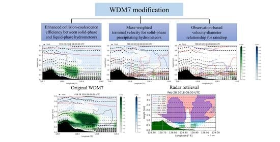
| CTL | WDM7 cloud microphysics scheme |
| EFF | CTL, with increased collision-coalescence (C-C) efficiency |
| VAH | EFF, with mass-weighted terminal velocity of solid-phase precipitable hydrometeors |
| VDR | VAH, with modified fall velocity–diameter (V–D) relationship of raindrops |
| Symbol | Expression | Process | Symbol | Expression | Process |
|---|---|---|---|---|---|
| Praci | Pracs | ||||
| Piacr, Niacr | Psacr, Nsacr | ||||
| Psacw, Nsacw | Pracg | ||||
| Pgacw, Ngacw | Pgacr, Ngacr | ||||
| Phacw, Nhacw | Phacr, Nhacr |
| Process | Description | Process | Description |
|---|---|---|---|
| Paacw | Accretion of cloud water by snow/graupel/hail | Prevs | Evaporation rate of rain to form cloud water |
| Pcact | Activation of cloud condensation nuclei | Psaci | Accretion of cloud ice by snow |
| Pcond | Condensation/evaporation of cloud water | Psacr | Accretion of rain by snow |
| Pgaut | Autoconversion of snow to form graupel | Psaut | Autoconversion of cloud ice to form snow |
| Pgaci | Accretion of cloud ice by graupel | Psdep | Deposition-sublimation rate of snow |
| Pgacr | Accretion of rain by graupel | Pseml | Enhanced melting rate of snow |
| Pgdep | Deposition-sublimation rate of graupel | Psevp | Evaporation of melting snow |
| Pgeml | Enhanced melting rate of graupel | Psmlt | Melting of snow to form rain |
| Pgevp | Evaporation of melting graupel | Naacw | Generation rate by accretion of cloud water snow/graupel/hail |
| Pgfrz | Freezing of rainwater to graupel | Ncact | Generation rate by activation of the CCN |
| Pgmlt | Melting of graupel to form rain | Nccol | Generation rate by self-collection of cloud water |
| Phaut | Autoconversion of graupel to form hail | Ncevp | Generation rate by cloud water evaporation |
| Phaci | Accretion of cloud ice by hail | Ngacr | Generation rate by accretion of rainwater by graupel |
| Phacr | Accretion of rain by hail | Ngeml | Generation rate by enhanced melting of graupel |
| Phdep | Deposition-sublimation rate of hail | Ngprz | Generation rate by freezing of rainwater to graupel |
| Pheml | Enhanced melting rate of hail | Ngmlt | Generation rate by melting graupel |
| Phevp | Evaporation of melting hail | Nhacr | Generation rate by accretion of rain water by hail |
| Phmlt | Melting of hail to form rain | Nheml | Generation rate by enhanced melting of hail |
| Piacr | Accretion of rain by cloud ice | Nhmlt | Generation rate by melting of hail |
| Pidep | Deposition-sublimation rate of cloud ice | Niacr | Generation rate by accretion of rain water by cloud ice |
| Pihmf | Homogeneous freezing of cloud water | Nihmf | Generation rate by homogeneous freezing |
| Pihtf | Heterogeneous freezing of cloud water | Nihtf | Generation rate by heterogeneous freezing |
| Pimlt | Instantaneous melting of cloud ice | Nimlt | Generation rate by melting cloud ice |
| Pigen | Generation (nucleation) of cloud ice from vapor | Nracw | Generation rate by accretion of cloud water by rain |
| Pracg | Accretion of graupel by rain | Nraut | Generation rate by autoconversion |
| Praci | Accretion of cloud ice by rain | Nrcol | Generation rate by self-collection of rain water |
| Pracs | Accretion of snow by rain | Nrevp | Generation rate by evaporation of rain water |
| Pracw | Accretion of cloud water by rain | Nsacr | Generation rate by accretion of rain water by snow |
| Praut | Autoconversion of cloud water | Nseml | Generation rate by enhanced melting of snow |
| Prevp | Evaporation-condensation rate of rain | Nsmlt | Generation rate by melting of snow |
| Name | POD | FAR | BIAS (mm) | ETS | PC | RMSE (mm) | Maximum Precipitation (mm) | |
|---|---|---|---|---|---|---|---|---|
| CASE1 | CTL | 0.708 | 0.286 | −3.34 | 0.05 | 0.55 | 10.09 | 50 |
| EFF | 0.782 | 0.277 | −3.85 | 0.08 | 0.60 | 10.02 | 60 | |
| VAH | 0.744 | 0.263 | −2.34 | 0.08 | 0.54 | 10.94 | 75 | |
| VDR | 0.750 | 0.265 | −2.24 | 0.08 | 0.54 | 11.03 | 77 | |
| CASE2 | CTL | 0.451 | 0.156 | −9.89 | 0.16 | 0.58 | 67.08 | 382 |
| EFF | 0.511 | 0.180 | 0.49 | 0.20 | 0.68 | 62.45 | 336 | |
| VAH | 0.475 | 0.152 | −8.98 | 0.18 | 0.66 | 62.28 | 335 | |
| VDR | 0.496 | 0.157 | −5.04 | 0.19 | 0.66 | 63.14 | 394 |
Publisher’s Note: MDPI stays neutral with regard to jurisdictional claims in published maps and institutional affiliations. |
© 2021 by the authors. Licensee MDPI, Basel, Switzerland. This article is an open access article distributed under the terms and conditions of the Creative Commons Attribution (CC BY) license (https://creativecommons.org/licenses/by/4.0/).
Share and Cite
Jang, S.; Lim, K.-S.S.; Ko, J.; Kim, K.; Lee, G.; Cho, S.-J.; Ahn, K.-D.; Lee, Y.-H. Revision of WDM7 Microphysics Scheme and Evaluation for Precipitating Convection over the Korean Peninsula. Remote Sens. 2021, 13, 3860. https://doi.org/10.3390/rs13193860
Jang S, Lim K-SS, Ko J, Kim K, Lee G, Cho S-J, Ahn K-D, Lee Y-H. Revision of WDM7 Microphysics Scheme and Evaluation for Precipitating Convection over the Korean Peninsula. Remote Sensing. 2021; 13(19):3860. https://doi.org/10.3390/rs13193860
Chicago/Turabian StyleJang, Sungbin, Kyo-Sun Sunny Lim, Jeongsu Ko, Kwonil Kim, GyuWon Lee, Su-Jeong Cho, Kwang-Deuk Ahn, and Yong-Hee Lee. 2021. "Revision of WDM7 Microphysics Scheme and Evaluation for Precipitating Convection over the Korean Peninsula" Remote Sensing 13, no. 19: 3860. https://doi.org/10.3390/rs13193860