1. Introduction
Fields shape agricultural landscapes. As a result, their size and distribution can inform about agriculture mechanization [
1], human development, species richness [
2], resource allocation and economic planning [
3,
4,
5]. Beyond their value as ecological and economical indicators, precise knowledge of the field distribution can help stakeholders across the agricultural sector monitor and manage crop production by enabling field-based analytics [
6]. Unlike property boundaries, which are recorded in local council or title records, field boundaries are not historically recorded. As a result, digital services currently ask their users to manually draw their field, which is time-consuming and creates disincentives. The objective of this work is to provide hassle-free access to field boundary data for unlocking field-based applications and insights to the Australian land sector. Given the structuring role of fields in agricultural systems, procurement of field boundary data is essential for the development of modern digital agriculture services. Therefore, efficient tools to routinely generate and update field boundaries are relevant for actors across the data value chain so that they can generate value and useful insights.
Satellite, aerial and drone images are prime sources of data used to automatically generate field boundaries. Aside from manual digitization based on photo interpretation, field boundaries can automatically be extracted by four main types of methods. First, edge-based methods rely on filters to emphasize discontinuities in images, that is, where pixel values change rapidly [
7,
8,
9]. Second, contour-based methods generate curves that move within images to find object boundaries by minimizing some energy function [
10]. Third, object-based methods cluster pixels together (i.e., fields) based on their color similarity [
9]. Finally, because not all edges are of interest, model-based methods are trained to recognize specific image objects to emphasize certain edges and attenuate others. Models range from simple logistic regression [
11] to structured random forest [
12], or more sophisticated models such as convolutional neural networks [
6,
13,
14,
15,
16,
17]. Convolutional neural networks have proven particularly accurate because they can learn discriminative hierarchical contextual features from the input images. Thus, the focus of this study is on convolutional neural networks.
Several convolutional neural networks have been proposed to extract field boundaries. Their performance has been demonstrated in a range of cropping systems from smallholder [
17] to large-scale commercial cropping systems [
6], with <1 m data [
18] to 3 m [
16,
17], 10 and 30 m data [
6]. Typically, these convolutional neural networks are trained to predict the presence or absence of field boundaries for each image pixel, i.e., they perform semantic segmentation. However, there is evidence that jointly predicting the task of interest (boundaries) with related tasks (such as the field extent or the distance to the closest boundary) improves prediction accuracy [
19], a process known as multitasking. In fact, in a previous study, we demonstrated that multitask learning maintained a high accuracy level when transferred across resolutions, sensors, space and time without recalibration [
6]. Such high transferability informed clear guidelines to scale up to larger landscapes. This paper capitalizes and expands on these past results to demonstrate nationwide field boundary extraction.
Semantic segmentation models (and edge-based methods) do not necessarily yield closed boundaries, and additional post-processing is required to define regions with closed contours (and achieve instance segmentation). Examples of post-processing methods include globalized boundary probability estimates, growing contours, thresholding or object-based image analysis [
6,
17,
20,
21]. In addition, once boundaries are mapped, one still needs ancillary information to define where the fields are. For instance, Yan and Roy [
7] and Graesser and Ramankutty [
8] sourced that information from cropland and type maps. While end-to-end instance segmentation methods could extract closed field boundaries in one go, they have not been widely tested for field boundary detection. So far, post-processing solves the problem of open boundaries.
In this paper, we introduce a new method based on deep learning field boundary extraction and demonstrate its performance by extracting fields across Australia. Our method is called DECODE in reference to its three processing steps: DEtection, COnsolidation and DElinetation. Detection is achieved with a state-of-the-art deep convolutional neural network that jointly predicts the extent of the fields, their boundaries and the distance to the closest boundary from single-date images. Consolidation is achieved by averaging single-date predictions over the growing season, thereby integrating temporal cues. Finally, delineation of individual fields is done by post-processing the boundary mask using hierarchical watershed segmentation. Our specific contributions are:
A deep learning network, the
FracTAL ResUNet, tailored for the task of semantic segmentation of satellite images. In particular, our architecture is a multitasking encoder–decoder network, with the same backbone structure as in Waldner and Diakogiannis [
6]. The main difference is that we changed the residual building blocks with atrous convolutions with the newest
FracTAL ResNet building blocks.
FracTAL ResNet building blocks have been recently proposed as part of a change detection network that demonstrated state-of-the-art performance [
22];
Two field-level measures of uncertainty to characterize the semantic (assigning labels to pixels) and instance (grouping pixels together) uncertainty;
A framework to report and compare field-based accuracy metrics.
Put together, these elements provide an accurate, scalable and transferable framework to extract field boundaries from satellite imagery. To demonstrate the performance of DECODE, we extracted 1.7 million fields across Australia using Sentinel-2 images. Two FracTAL ResUNet models were compared: one trained with data of Australia (the target domain), and the other with data of South Africa (the source domain). As this paper will show, both models yielded accurate results in Australia, which is remarkable since no adjustments were applied to the source-to-target case. This is evidence that our approach generalizes well and can be transferred to other regions.
2. Materials and Methods
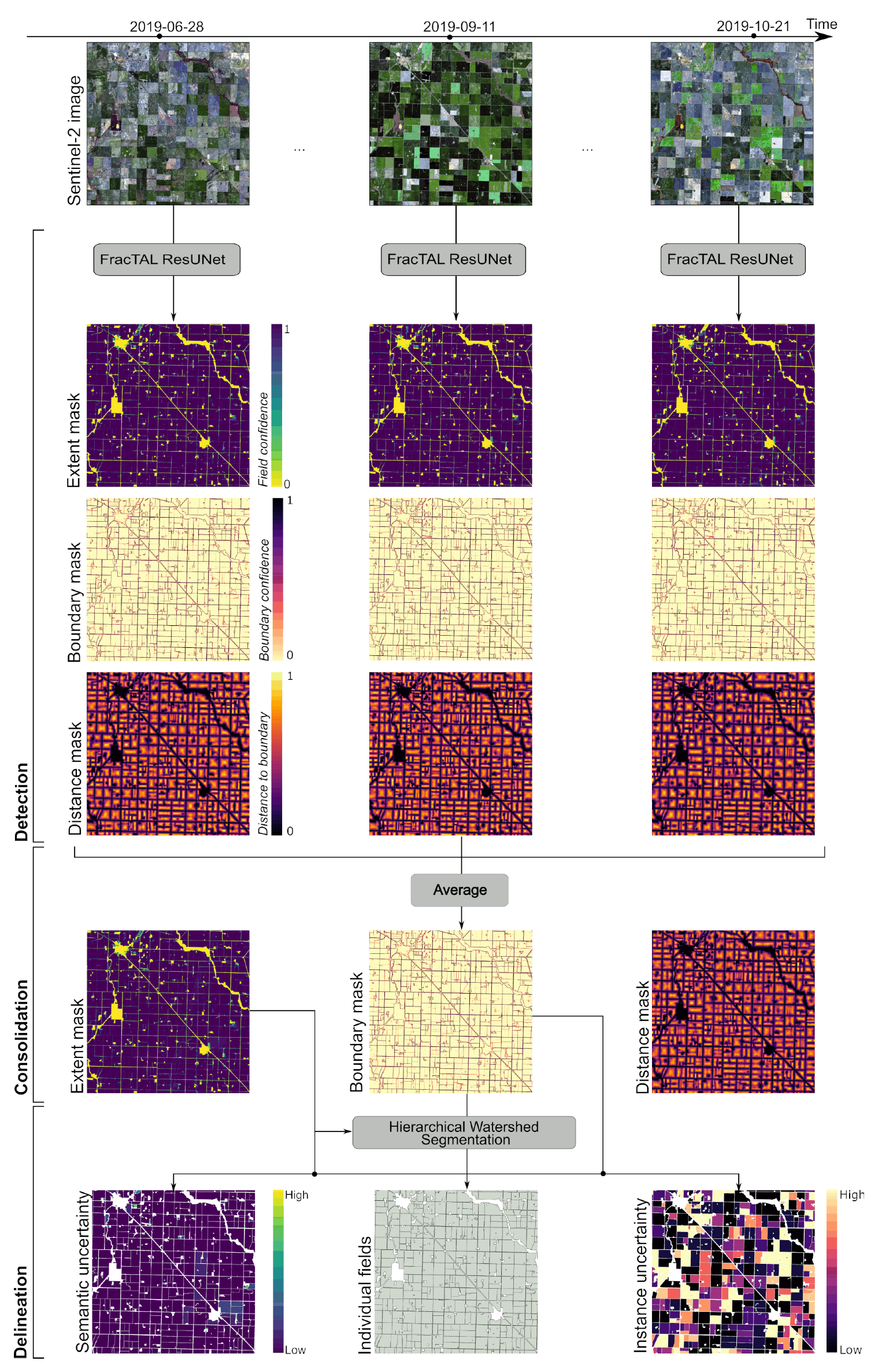
The
DECODE method extracts field boundaries from satellite imagery in three sequential steps (
Figure 1). The first step (detect) is a semantic segmentation step, where a convolutional neural network,
FracTAL ResUNet, assigns multiple labels (field presence, boundary presence and distance to boundary) to image pixels (
Section 2.1). The second step (consolidate) averages model predictions obtained for different observation dates so that temporal cues are integrated (
Section 2.2). This creates consolidated model predictions from which individual fields can be extracted. The third and final step (delineate) is an instance segmentation step, where image pixels are grouped into individual objects (fields) based on the consolidated network predictions (
Section 2.3). During this process, two uncertainty metrics—one that relates to the semantic segmentation step and the other to the instance segmentation step—are computed for each field. Code is available on
https://github.com/waldnerf/decode (accessed on 3 May 2021).
2.1. Detect: Multi-Task Semantic Segmentation
Semantic segmentation has attracted significant interest in the fields of computer vision and remote sensing, where automatically annotating images is common. In the next paragraphs, we summarize the main contributions leading to this work and we refer to Brodrick et al. [
23] for a thorough introduction to convolutional neural networks.
The UNet architecture [
24], which introduced the encoder–decoder paradigm, made major breakthroughs in image semantic segmentation. The encoder encodes the input image into feature representations at multiple levels through a series of convolutions, activation functions (such as ReLU activations) and pooling layers. The decoder semantically projects the discriminative features learnt by the encoder onto the pixel space to derive a dense classification through a series of upsampling, concatenation and convolution operations. As networks became increasingly deeper, they became more difficult to train due to vanishing (or exploding) gradients. Residual networks (
ResNets) [
25] mitigate this problem by introducing skip connections to allow gradient information to pass through layers. As a result, information from the earlier parts of the network flows to the deeper parts, helping maintain signal propagation. Pyramid scene parsing pooling (PSP pooling) [
26] was introduced to capture the global context in the image, which helps models classify the pixels based on the global information present in the image. In PSP pooling layers, the feature map is pooled at different scales before passing through a convolution layer. Then, the pooled features are upsampled to make them the same size as the original feature map. Finally, the upsampled maps and the original feature map are concatenated and passed to the decoder. This technique fuses the features at different scales, hence aggregating the overall context. Multitasking, where multiple tasks are simultaneously learned by a model, is another approach to improving generalization. The
UNet, residual connections, pyramid scene parsing pooling, and multi-tasking inference were combined in
ResUnet-a and showed state-of-the-art performance on very high resolution aerial images [
19].
In recent years, attention mechanisms have improved the success of various deep learning models, and continue to be omnipresent in state-of-the-art models. One of those attention mechanisms is self-attention, which quantifies the interdependence within the input elements. Self-attention is a form of “memory” acquired during the training of a network that helps emphasize important features in convolution layers. It was pioneered in the task of neural machine translation [
27] where it helped emphasize important words, as well as their relative syntax between different languages, in long sentences. It has been shown consistently to improve performance and it is now a standard in all modern architectures e.g., [
28]. Self-attention layers can be combined in multi-head attention layers that jointly learn different representations from different positions. Among the attention modules that have been proposed, the fractal Tanimoto attention layer is memory efficient and scales well with the size of input features. It uses the fractal Tanimoto similarity coefficient as a means of quantifying the similarity between query and key entries.
FracTAL ResNet blocks have a small memory footprint and excellent convergence and performance properties that outperform standard
ResNet building blocks; see [
22] for more details.
In this paper, we introduce
FracTAL ResUNet, a convolutional neural network that is largely based on
ResUnet-a [
19] but where the atrous
ResNet blocks are replaced by the more efficient
FracTAL ResNet blocks. In the next sections, we describe
FracTAL ResUNet in terms of its micro-topology (feature extraction units), macro-topology (backbone) and classification head.
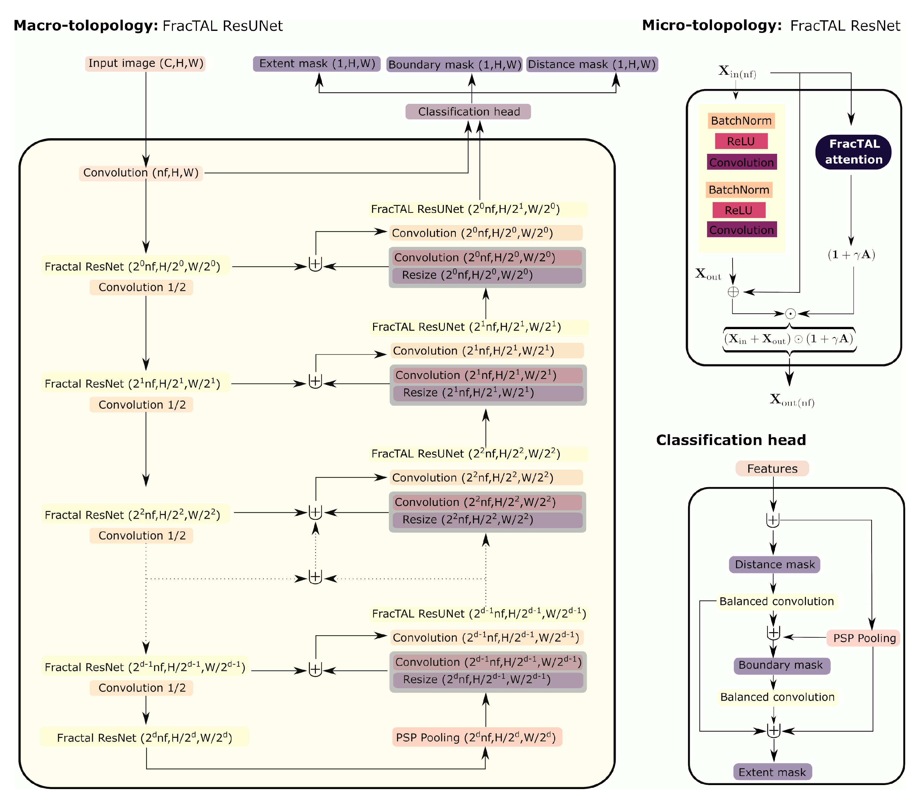
2.1.1. Architecture Micro-Topology
The founding block used for this paper is the
FracTAL ResNet unit [
22]. It consists of the standard sequence one finds in residual building blocks enhanced by a
FracTAL unit (i.e., a channel and spatial self-attention layer). In the
FracTAL ResNet, the order of operations is as follows: the input layer (
) is first subjected to the standard sequence of batch normalization,
ReLU activation and 2D convolution operations. This sequence produces an output layer (
). The input layer is also subject to the
FracTAL unit that produces a self-attention layer (
). The input, the output of the residual blocks and the attention layer are fused together with a learnable annealing parameter (
) initialized at zero when training starts:
Here, ⊙ designates elementwise multiplication. The summation
is what one obtains by using a standard residual unit [
29]. This residual output is emphasized in an annealing way by the attention layer,
. This unit has excellent performance but a small memory footprint, which is critical when dealing with deep architectures and large training data sets.
2.1.2. Architecture Macro-Topology
The feature extraction units were inserted in an encoder–decoder scheme similar to the
UNet architecture used in Diakogiannis et al. [
22] (
Figure 2). The input of the encoder is first processed by a normed convolution to bring the number of channels to the desired number of features (without activation). These features are then subjected to a set of
FracTAL ResNet units. Between
FracTAL ResNet units, the size of the spatial extent is halved and the number of filters doubled. This is achieved with a normed convolution of stride (
s = 2; without activation). At the end of the encoder, we apply the pyramid scene parsing pooling operator [
30]. This operator provides context information at different scales of the spatial dimensions of the input features (successively, 1, 1/2, 1/4, 1/8) and has been shown to improve performance. In the decoder, features are upscaled using bilinear interpolation followed by a normed convolution. At each level, the upscaled features are first concatenated with the encoder features of the same level. Next, a normed convolution brings these features to a desired size and the output is inserted into the next
FracTAL ResNet unit. The final layer of the decoder, as well as the output of the first convolution layer, are the inputs to the classification head.
2.1.3. Classification Head
The classification head follows conditioned multitasking [
6,
19] and is identical to the one presented in Diakogiannis et al. [
22]. It first predicts the presence of field boundaries (i.e., the boundary mask). Then, it balances the boundary mask and re-uses it to estimate the distance to the closest field boundary (i.e., distance transform). Here, “balanced” means that the number of output channels (e.g., of the distance mask) was changed to correspond to the number of channels of the input features (usually 32). This scheme weights intermediate prediction layers and feature layers equally, thereby counterbalancing the lesser number of channels in the former. Finally, it re-uses both previous outputs to map the presence or absence of fields (i.e., the extent mask). The number of features in each of these layers was carefully balanced in each of these layers and, for the case of boundaries prediction, a scaled sigmoid activation was introduced, as this sharpens the boundary predictions.
2.1.4. Evolving Loss Strategy
Our training loss was the fractal Tanimoto with complement loss [
22]. Assuming that
represents one of the predictions of the network (i.e., it is a fuzzy binary vector) and
represents the ground truth labels, then the fractal Tanimoto similarity coefficient is defined through:
where:
Here d, represents the depth of the iteration in the fractal definition. The higher the value of d, the finer the similarity between predictions and labels.
This similarity coefficient takes the value 1 when
(predictions are perfect) and zero when
(no correlation between predictions and ground truth labels). The loss can be defined for minimization problems as the negative of this coefficient:
In this formulation, the loss function admits values in the range
. As we optimized three learning tasks jointly, the full loss function was defined as the average of the loss of all tasks:
The training procedure we followed was the evolving loss strategy [
22]: starting from fractal depth
and an initial learning rate,
lr=1.e-3, we increased the depth of the fractal Tanimoto loss each time we reduced the learning rate (
Section 2.5.2). This training scheme helps avoid local minima by making the loss landscape steeper towards optimality. It has been shown to improve all statistical metrics; for the case of intersection over union, the improvement was ∼1% performance [
22].
2.2. Consolidate: Time Averaging
The outputs of the deep-learning model are three semantic segmentation layers per input image. The consolidate step aims at consolidating single-date predictions while maintaining flexibility (the method still works with a single image). Averaging across observations also significantly increases accuracy, especially when more than four observations are available [
6].
2.3. Delineate: Hierarchical Watershed Segmentation
The outputs of the consolidate step are thus three consolidated semantic segmentation layers but individual fields remain to be defined. We achieve instance segmentation by post-processing the boundary mask using hierarchical watershed segmentation.
2.3.1. Hierarchical Watershed Segmentation
Watershed segmentation is one of the most popular image segmentation methods. Consider a grey-scale image as a topographic surface; pixel values correspond to elevation. Valleys appear in dark grays and mountain tops and crest lines appear in light grays. Following the drop of water principle [
31], watersheds are defined as groups of pixels from which a drop of water can flow down towards distinct minima.
This intuitive idea has been formalized for defining a watershed of an edge-weighted graph [
32]. The graph
G is defined as a pair (
P,
E) where
P is a finite set and
E is composed of unordered pairs of distinct elements in
P [
33]. Each element of
P is an image pixel, and each element of
E is called an edge. The graph
G models the image spatial domain:
P is the regular 2D grid of pixels and
E is the
or
adjacency relation. Spatial relations have different weights
W that the dissimilarity between pixels, so that (
G,
W) is an edge-weighted graph. A segmentation
of
P is then defined as a subset of
V such that the intersection of any two distinct instances of
is empty, and the union of instances of
equals
V. Thus, one can obtain a sequence of nested segmentations, hence a hierarchy of segmentations.
A hierarchy of watershed segmentations is a nested sequence of coarse to fine instances, which can be shown as a tree of regions [
32,
34]. Therefore, coarser to finer image instances or objects can be obtained by cutting the hierarchy lower or higher in the tree.
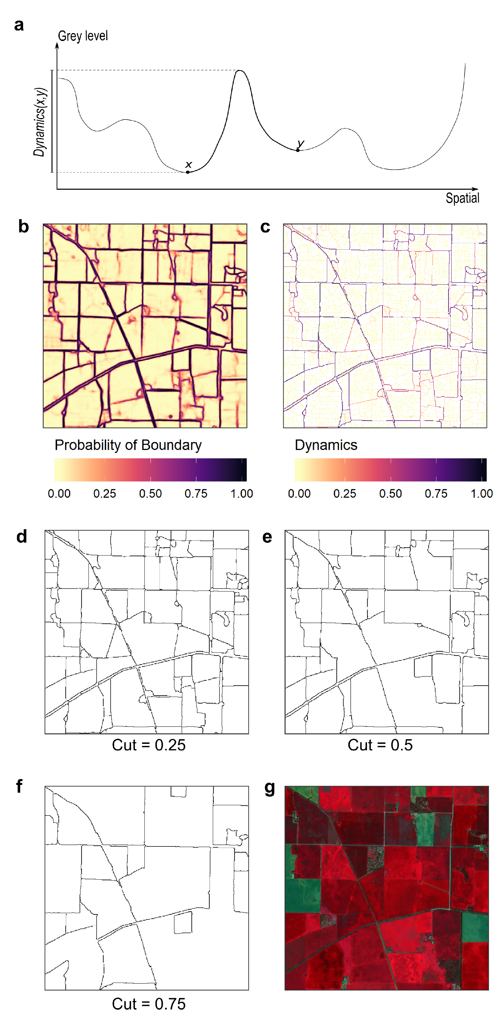
2.3.2. Closing Boundaries with Hierarchical Watershed Segmentation
Instance segmentation can be obtained by cutting hierarchical watershed segmentations into
k regions at any level of the hierarchy [
32]. The resulting segments will have closed boundaries regardless of the threshold use to cut the hierarchy. In this paper, we built a watershed hierarchy based on the boundary mask (
Figure 3b,d–f). The weights of the graph edges were measured by their dynamics [
35]. The dynamics of a path that links two pixels is the difference in altitude between the points of highest and lowest altitude of the path (
Figure 3a). In an image, the dynamics of two pixels is equal to the dynamics of the path with the lowest dynamics (
Figure 3c). Once the edge-weighted graph is generated from the boundary mask, instances fields with closed boundaries can be generated by cutting the graph at a specific dynamics (
).
Before constructing the watershed hierarchy, we set another threshold () to binarize the extent mask and define field pixels and non-field pixels. The value of non-field pixels in the boundary mask is then changed to 1, which corresponds to the maximum confidence of having a boundary. This step reduces the occurrence of very small fields. We finally construct the watershed hierarchy and cut it at the desired level. Here, and were defined by trial and error and set to 0.2 and 0.4, respectively.
2.4. Defining Semantic and Instance Uncertainty
Two types of uncertainty can be characterized for each field: the uncertainty related to the identification of the fields (semantic uncertainty) and the uncertainty related to their delineation (instance uncertainty).
We propose to measure semantic uncertainty using the extent mask, which describes the probability of a pixel to belong to a field. Semantic uncertainty is defined as the average normalized difference between the extent probabilities of all pixels in a field and the threshold value:
where
ranges between 0 and 1 and values close to 1 indicate a high uncertainty of the detection process.
Fields must have closed boundaries. Confidence in these boundaries relates to the uncertainty of the pixels making up these boundaries. We propose to measure instance uncertainty using the concept of dynamics that was introduced previously. Pixels with high dynamics were identified as boundary pixels with high confidence, and conversely for low dynamics. Therefore, if
defines the ensemble of boundary pixels of a specific field, instance uncertainty can be derived from the boundary pixel with the lowest dynamics (i.e., the weakest link between boundary pixels):
where
ranges between 0 and 1 and values close to 1 indicate a high uncertainty of the delineation process.
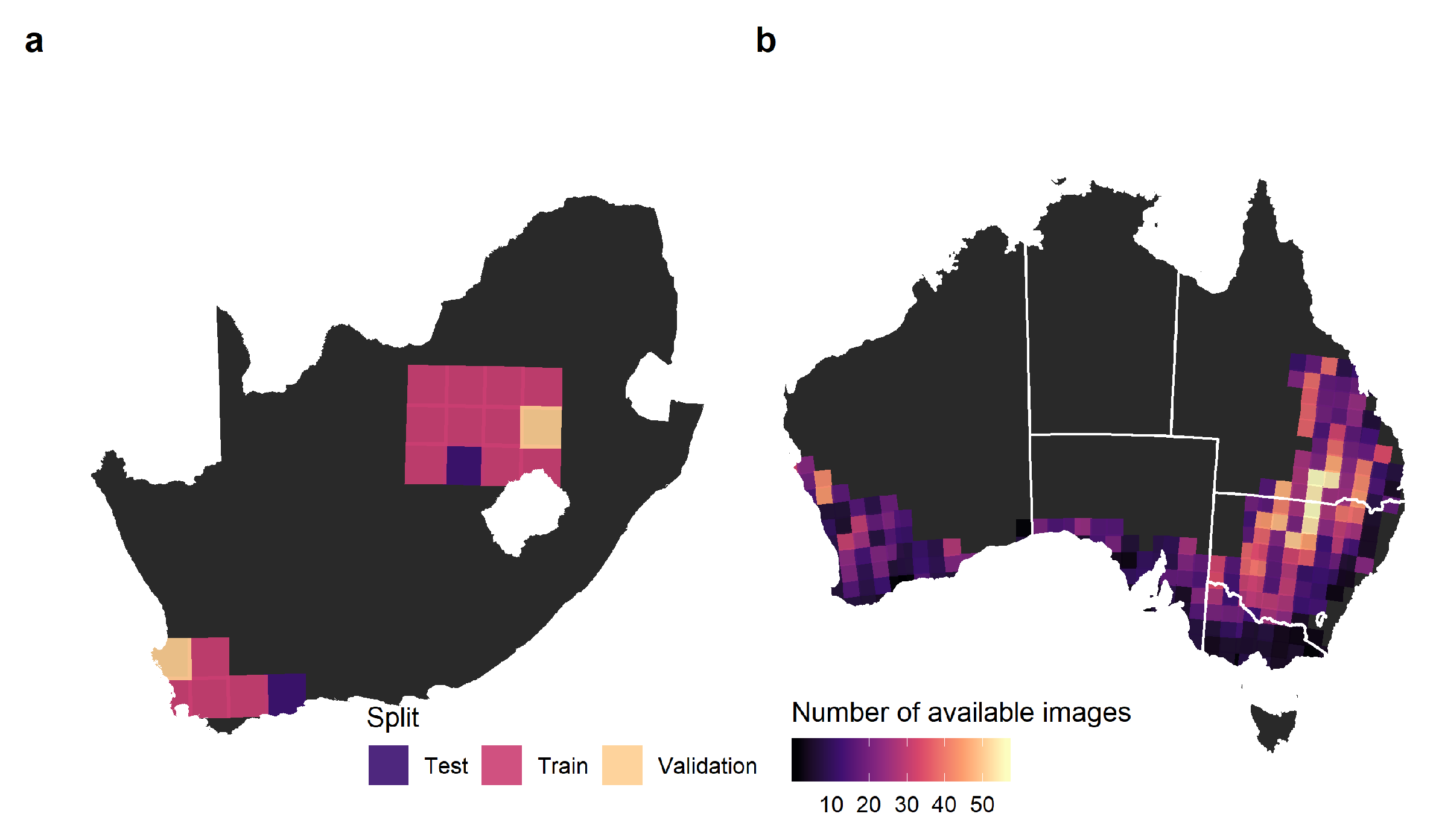
2.5. Experimental Design
We evaluated the
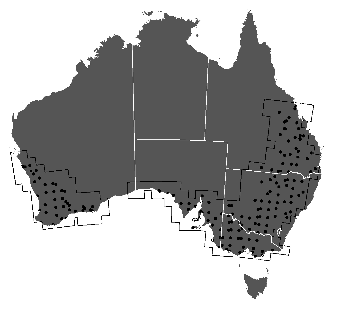
DECODE method by extracting field boundaries across the Australian grains zone (
Figure 4) and trained a first
FracTAL ResUNet model using data from Australia (the target domain). We also trained a second model using data from South Africa (the source domain) to assess its transferability. We note that the fields in these countries have some similarity in size and shapes. To better understand how transferable models trained on different domains are, we compared the following two cases:
Target to target, where a FracTAL ResUNet model was trained and evaluated on data from Australia (the target domain);
Source to target, where a FracTAL ResUNet model was trained on data from South Africa (the source domain) and evaluated in Australia.
While the source-to-source case (where a FracTAL ResUNet model was trained and evaluated on data from South Africa) was not our primary focus, it provides an interesting benchmark and is thus included in some analyses.
2.5.1. Data and Study Sites
We had two study sites in South Africa: one in the “Maize quadrangle”, which spans across the major maize-producing area; and the other in the Western Free State. These sites cover 18 Sentinel-2 tiles: 14 tiles were used for training, two for validating and two for testing. In practice, the two testing sites were only used to provide informative accuracy measures. Two cloud-free images were available per tile, one early (aiming for February) and the other late in the season (aiming for May;
Table A1). They were partitioned into a set of smaller images (hereafter referred to as input images) of a size of 256 × 256 pixels because entire images cannot be process at once due to limited GPU memory. As in Waldner and Diakogiannis [
6], we kept the blue, green, red and near-infrared bands.
We sourced boundaries that were created by manually digitizing all fields throughout the country based on 2.5 m resolution, pan-merged SPOT imagery acquired between 2015 and 2017. About 380,000 fields were available for training, 65,000 for validation and 35,000 for testing (
Table 1). We rasterized field polygons at 10 m pixel resolution so as to match Sentinel-2’s grid, providing a rich wall-to-wall data set. We finally created the three annotated masks needed by
FracTAL ResUNet during training: the extent mask (binary), the boundary mask (binary; a 10 m buffer was applied), and the distance mask (continuous), representing, for every within-field pixel, the distance to the closest boundary. Distances were normalized per field so that the largest distance was always one. As boundaries are updated every three years, discrepancies might exist between them and those seen on Sentinel-2 images. While these discrepancies might be handled during the training phase, their impact is far greater in accuracy assessment. Therefore, accuracy measures for the source-to-source approach remain indicative.
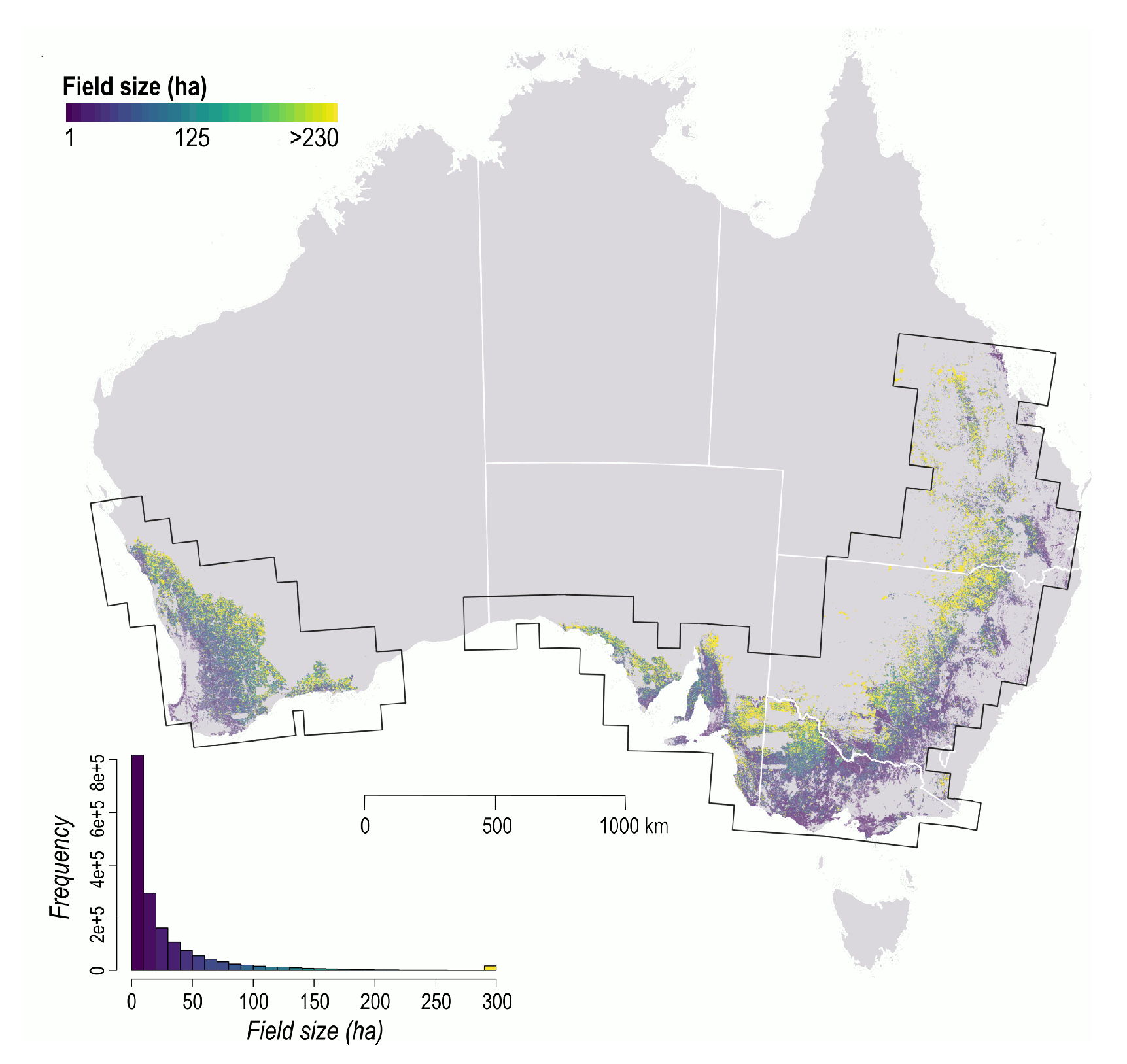
In Australia, we downloaded 5302 cloud-free images across 269 tiles (
Figure 4). Partial images due to orbital tracks were discarded if complete images were also available from other orbits. The median number of available images per tile was 14, ranging from a maximum of 56 (55JEH and 55JEK) to a minimum of 1 (50HQH, 50JKM, 51HTC, 52JDL, 53HMB, 53HPA, 54HYC and 55HFU), totaling more than 500 million 10 m pixels.
Field boundaries for training and testing in Australia were generated differently because of their different requirements. On the one hand, training requires a large amount of contiguous data representative of the variety of landscapes and can tolerate some level of noise. On the other hand, testing requires fewer data points but quality control and sampling design are critical. Therefore, field boundaries for training were generated by a two-step process where operators edited objects generated by an image segmentation method while field boundaries for testing were manually digitized. Field boundaries for training were obtained from five tiles (55HEE, 55HDA, 54HXE, 53HNC and 50JPL) for which two cloud-free dates were available. First, we extracted the first five components of these images using principal component analysis and non-cropped areas were masked using the Catchment-scale Land-Use of Australia Map (CLUM) [
36]. Next, we extracted field polygons using a meanshift segmentation algorithm [
37]. To define the optimal segmentation parameters, Bayesian optimization [
38] was used to minimize over- and under-segmentation, which were measured by comparison of the segmentation outputs to 200 randomly drawn fields. The resulting polygons were then reviewed, deleted, added or corrected manually using all of the Sentinel-2 images available as well as Google Earth. Editing reduced the number of polygons by up to 80% depending on the tile, which illustrates the challenge that lies in calibrating object-based methods. As a result, more than 50,000 and 10,000 fields were available for training and validation, respectively. Test data were manually digitized by photo-interpreting Sentinel-2 images (
Table 1). To define the sampling locations, Sentinel-2 tiles were split into chips of 2.5 by 2.5 km and their respective crop proportions were computed based on CLUM. Then, we randomly selected one of these chips per tile. Tiles where all chips had less than 10% cropping were ignored. Finally, photo-interpreters labelled 176 well-distributed chips (
Figure A1), resulting in 5555 test fields.
2.5.2. Model Training
FracTAL ResUNet models were trained by feeding input images (with the shape 256 pixels × 256 pixels × 4 spectral bands) to the network and comparing their three output masks (extent, boundary and distance) to the reference masks generated as explained in the previous section. In all experiments, our models had the following hyperparameters: 32 initial filters, a depth of 6, a width of 1, and a PSP pooling depth of 4. We also set the depth of the
FracTAL attention layer to 5. We initialized the model weights using Xavier initialization [
39] and used Adam as the optimizer because it achieves faster convergence than other alternatives [
40]. We followed the parameter settings recommended in Kingma and Ba [
40]. Training was initiated with the standard Tanimoto loss (
). Then, we increased the depth
d of the fractal Tanimoto loss each time we reduced the learning rate (when training converges). We chose the following sets of values for the various learning rate (
) reduction steps:
,
,
,
.
Data augmentation artificially inflates the variance of training data, which boosts the ability of convolutional neural networks to generalize. Indeed, convolutional neural networks, and specifically
UNets, are not equivariant to spatial transformations such as scaling and rotation [
41]. Therefore, during training, we flipped the original images (in the horizontal and vertical reflections) and randomly modified their brightness. This means the network never exactly saw the same data during training. We also performed temporal data augmentation as we used the same labels for multiple image dates.
2.5.3. Large-Scale Instance Segmentation
Instance segmentation was performed per tile to minimize memory usage and allow distributed computing. To combine fields from multiple overlapping tiles into a seamless, continuous data layer, we implemented the following two rules. First, all fields touching the tiles’ bounding box were discarded because they were most likely incomplete. Second, in overlap areas between tiles, we retained the field with the lowest instance uncertainty.
2.5.4. Accuracy Assessment
When characterizing the accuracy of extracted field boundaries, both the geometric and thematic accuracy must be assessed. Thematic accuracy is computed at the pixel level and is expressed by common metrics derived from the error matrix. Here, we report the overall accuracy, the users’ accuracy, the producers’ accuracy [
42] and Matthews’ correlation coefficient (MCC; [
43]) of the extent mask.
Geometric accuracy is computed at the instance level and can be broken down into four components parts—similarity in shape, label, contour and location, each depicting a specific view of the similarity between reference and extracted fields. We report six geometric accuracy metrics:
The boundary similarity, which compares the boundary of a reference object coincident with that of a classified object [
44]. Boundary similarity calculates the percentage of the target field boundary that coincides with the extracted field boundary:
where
is the length of the point set intersection between the boundaries of the target and extracted fields, and
k is +1 when
is less than or equal to
, and −1 otherwise.
The location similarity, which evaluates the similarity between the centroid position of classified and reference objects [
44]. Location similarity is evaluated first, by calculating the Euclidiean distance between corresponding the centroids of the target and extracted fields, and then by normalizing it by the diameter of a combined area circle (
), i.e., the diameter of a circle whose area corresponds to the sum of the areas of the target and extracted fields:
where
d is a function that computes the Euclidian distance between the centroids of the reference field (
) and the corresponding extracted field(s) (
), and
is the diameter of the combined area circle.
The oversegmentation rate, which measures incorrect subdivision of larger objects into smaller ones:
where
is an operator that calculates the area of a field from
E or
T and ∩ is the intersection operator.
The undersegmentation rate, which measures incorrect consolidation of small adjacent objects into larger ones [
45]:
The intersection over union, which evaluates the overlap between reference and classified objects;
The shape similarity, which compares the geometric form of a reference object with that of the corresponding classified object(s) [
44]. Shape similarity is based on the normalized perimeter index (
) and the concept of an equal area circle (
), which is a circle with an area equal to the area of an object (here a field). The
of an object is in fact the ratio between the perimeter of the equal area circle and the perimeter of the object (
). Here, shape similarity compares the geometric form of a target field with that of the corresponding extracted field(s):
where
k is given the value +1 when
is less than or equal to 1.0, and the value –1 otherwise.
All of these metrics were defined to range between 0 and 1; the closer to 1, the more accurate. If an extracted field intersected with more than one field in T, metrics were weighted by the corresponding intersection areas.
As object-based metrics are available for all reference fields, we introduce the concept of the Area Under the Probability of Exceedance Curve (AUPEC) to facilitate comparison between methods and provide a synoptic summary of a method’s performance. Probability of exceedance curve is a common type of chart that gives the probability (vertical axis) that an accuracy level (horizontal axis) will be exceeded. To illustrate this concept, let us consider a probability of exceedance of 50% for an accuracy level of 0.9. This indicates that every second reference field has an accuracy value of at least 0.9. As perfectly extracted fields have an accuracy value of 1, perfect segmentation for the full reference data set should yield a probability of exceedance of 100% for an accuracy of 1 and a probability of exceedance of 100%. It follows that the area under the probability of exceedance curve summarizes the distribution of accuracy of the reference data. An area under the probability of exceedance curve close to 1 indicates that nearly all extracted fields were error-free for the metric considered, and conversely for values close to 0.
3. Results
To extract fields in Australia, we trained two
FracTAL ResUNet models: one model with data from South Africa (source-to-target) and the other with data from Australia (target-to-target). Training lasted for 72 h per model, using 24 nodes equipped with 4 P100 GPUs and 16 GB of memory each. Optimal training was achieved after 254 epochs for the model trained on data from South Africa (MCC = 0.85) and 161 epochs for the model trained on data from Australia (MCC = 0.87). Inference for Australia ran for 5 days on 16 to 24 nodes, each having 4 P100 GPUs and 128 GB of memory. About 1.7 million fields (>1 ha) were extracted with both methods (
Figure 5).
We then assessed the pixel-based accuracy of both models in the target domain (
Table 2). Overall, the source-to-target and target-to-target approaches yielded similar accuracy levels (0.87). The target-to-target approach yielded larger producers’ accuracy than the source-to-target approach (0.83 vs. 0.78) but this was achieved at the expense of the field class (0.90 vs. 0.94). Users’ accuracy for both approaches and classes was >0.85.
Visual inspection of the extent, boundary and extent masks confirmed the good performance of the source-to-target approach across a range of cropping regions (
Figure 6). The model showed great confidence in detecting fields regardless of the fragmentation levels. Most errors were observed in southern Queensland and central and northern New South Wales, which were stricken by drought during the period of interest. As a result, separability with other natural vegetation classes was reduced. Checker-board artifacts in the semantic segmentation outputs were largely avoided thanks to our specific inference method.
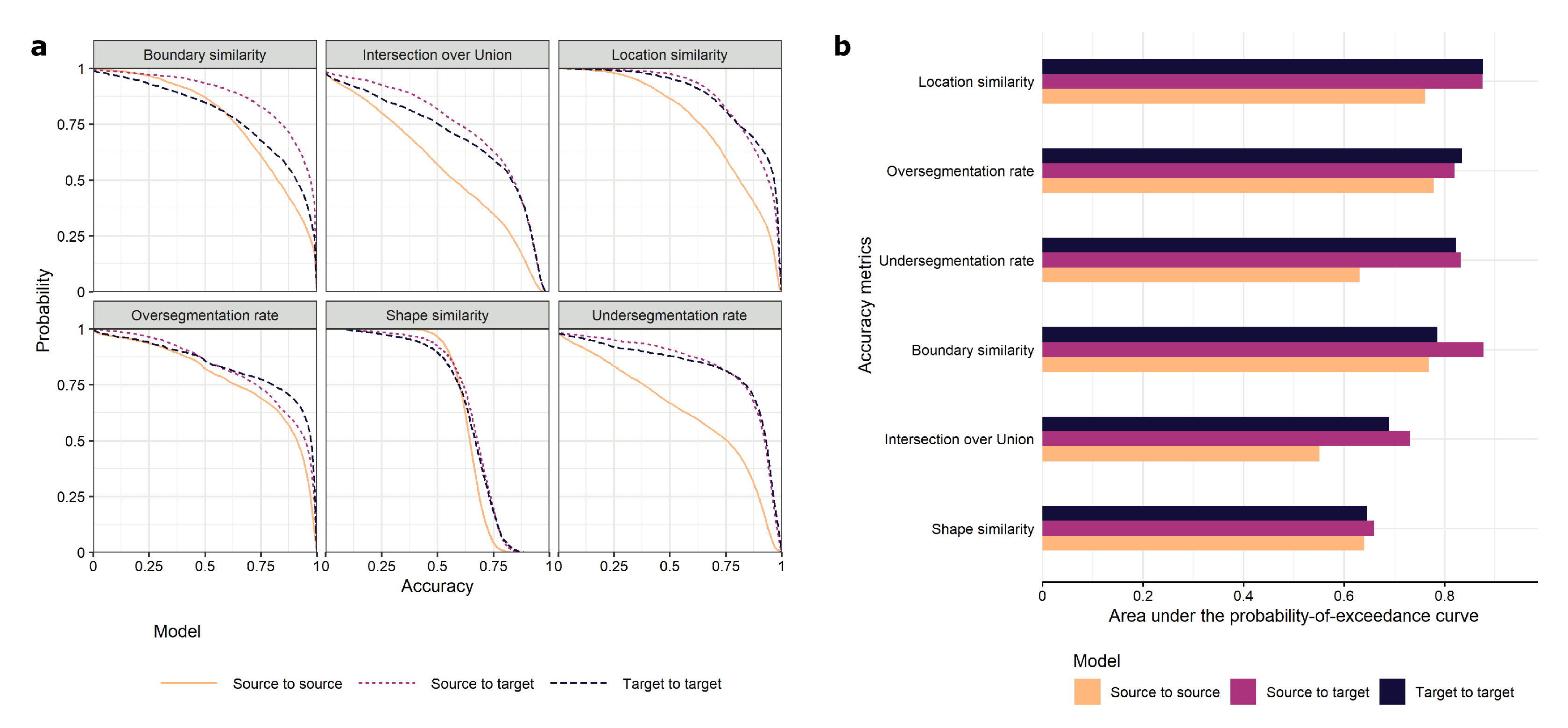
We then evaluated object-based accuracy based on six metrics (boundary similarity, intersection over union, location similarity, oversegmentation rate, shape similarity and undersegmentation rate). We compared the source-to-target and the target-to-target approaches based on the probability of exceedance curves and their associated areas under the curves (
Figure 7a). Even though they are not directly comparable, we also included the accuracy metrics for source-to-source results for reference.
Extracted fields were very similar to reference fields across metrics and approaches. In particular, they had high location similarity and over/undersegmentation rates. For example, 75% of the extracted fields reached an over/undersegmentation rate of at least 0.75. Shape similarity was the poorest metric, with 50% of the fields yielding to a similarity of 0.6. Surprisingly, the source-to-target approach outperformed the target-to-target approach for most metrics (
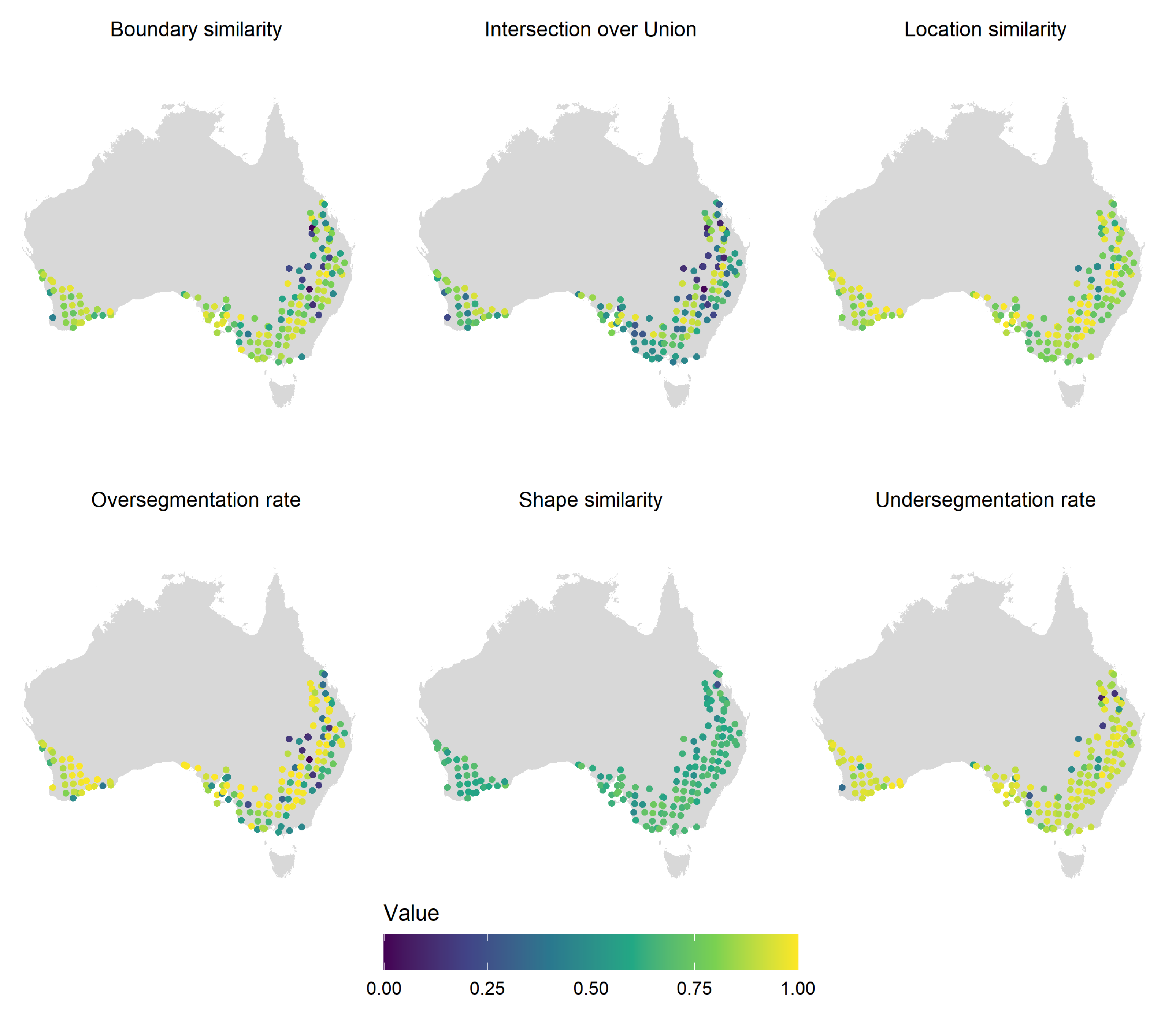
Figure 7b). The largest differences in areas under the probability of exceedance curves were observed for boundary similarity (0.89 vs. 0.79). The larger size of the source training set data might have exposed the model to a larger diversity of cases, leading to improved accuracy. Poor performance in the source-to-source case was likely due to discrepancies between the observation date and the reference. While the shape and undersegmentation errors seemed relatively evenly distributed, oversegmentation and location errors tended to decrease in low rainfall zones (more inland) where pasture fields are less prevalent (
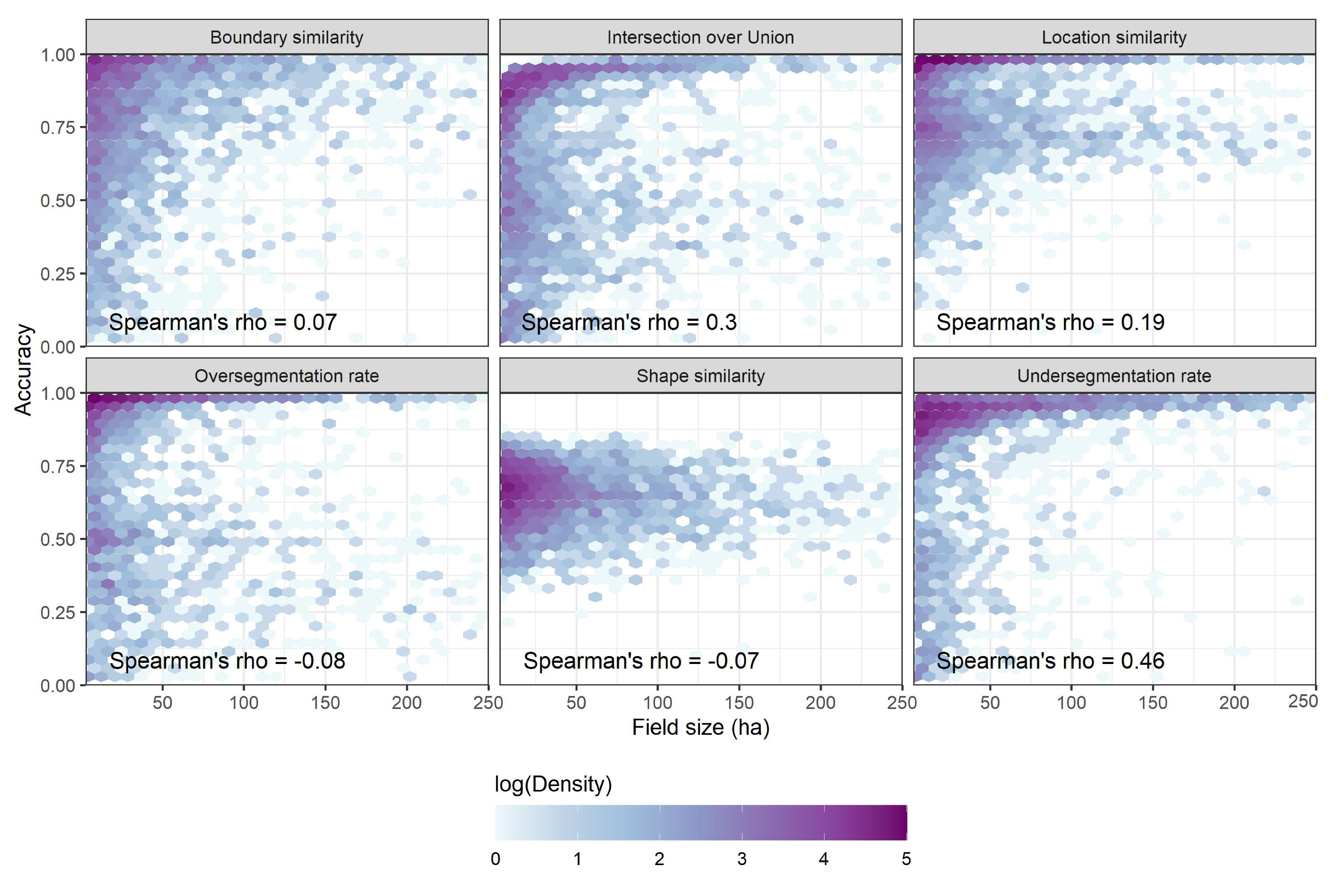
Figure 8). The undersegmentation rate and intersection over union increased as field size grew larger. The other accuracy metrics did not indicate any strong relationship with field size (
Figure A2).
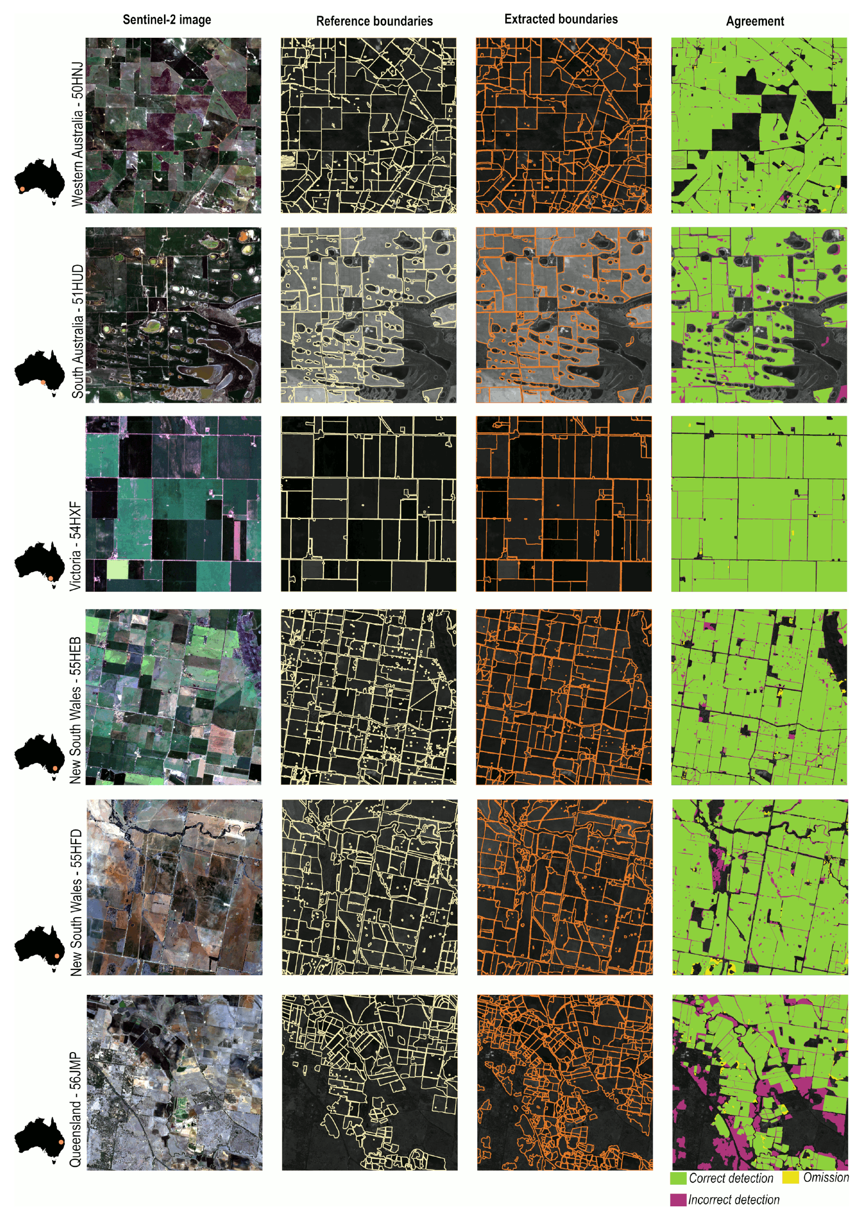
Again, visual assessment confirmed the results of the quantitative accuracy assessment (
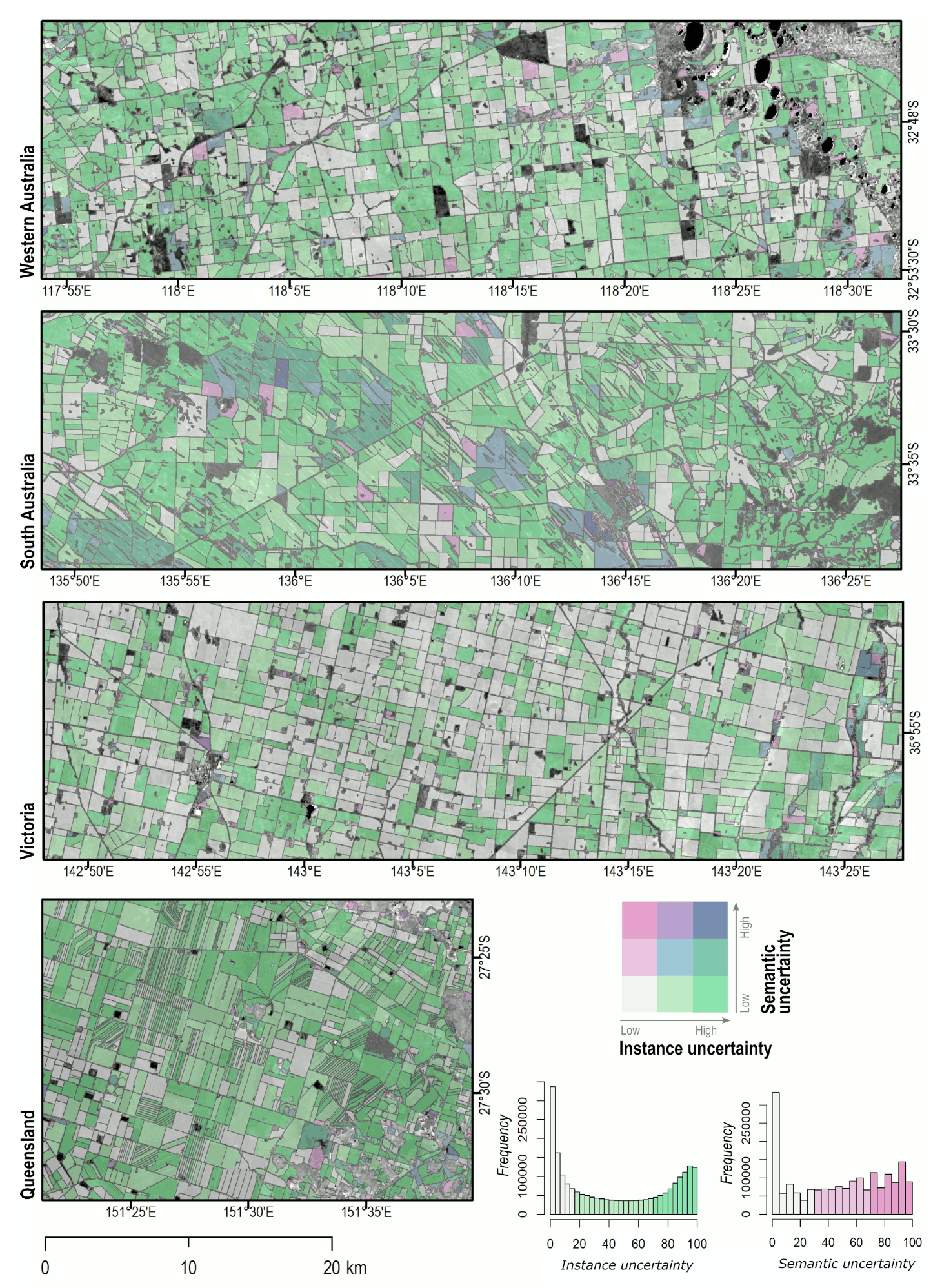
Figure 9). Our method showed good performance across agricultural landscapes. For instance, it delineated fields with high fidelity and accuracy, even in the more complex landscapes (e.g., South Australia and Queensland). It also successfully retrieved fields with interior boundaries (e.g., lakes, tree lines, buildings) and in areas where crop cover was sparse (New South Wales and Queensland). This suggests that our method still yields good results in the absence of peak season images. Nonetheless, the large number of small fields (<10 ha) suggests that a non-negligible proportion of those is erroneous. Confidence in the extracted fields can also rapidly communicate the uncertainty related to the field extraction process (
Figure 10).
4. Discussion
4.1. Methodological Advancement and Their Relevance
In this paper, we taught machines to delineate field boundaries according to spatial, spectral and temporal properties. To demonstrate the performance of our method, DECODE, we have processed >200 billion Sentinel-2 pixels across the Australian grains zone from which we extracted about 1.7 million fields. As input images are single-date observations, field boundaries can be updated at any time in the season according to users’ needs.
Convolutional neural networks have pushed the boundaries of boundary detection [
46]. In this paper, we addressed the problem of satellite-based delineation of field boundaries as multiple semantic segmentation tasks, resulting in excellent performance both at the pixel level and the field level. This is because neural networks learn to discard edges that are not part of field boundaries and to emphasize those that are using spectral and multilevel contextual features that are relevant for multiple correlated tasks. As such, it confirms the results of previous studies that evaluated deep-learning for field boundaries extraction (e.g., Waldner and Diakogiannis [
6], Masoud et al. [
16], Persello et al. [
17]) but our contribution is unprecedented in scale. While our results show clear improvement over previous work, direct and fair comparison may be difficult for two main reasons. First, there are several differences in the experimental setup, such as the imagery data (resolution, spectral bands, multi-sensor, multi-date), the training set (size, proportion), the landscape complexity and fragmentation, or the extent of the area of interest. Second, field boundary extraction, unlike more land-use/land-cover classification tasks, lacks a shared protocol for evaluation. As a result, the variety of metrics reported, regardless of their merit, undermines comparison. This highlights the need for common data sets as well as a shared set of evaluation metrics to allow systematic method benchmarking.
FracTAL ResUNet demonstrated excellent generalization and transfer properties. The greater accuracy level shown by the source-to-target approach over the target-to-target approach clearly evidences its excellent transferability. We believe that three factors help explain this behavior. First, learning from multiple, correlated tasks is pivotal to minimize over-fitting and achieve high generalization. Using this strategy, we showed in an earlier contribution that models could generalize and transfer across space, time and resolution [
6]. Second, we included target-domain images and source-domain images when computing the standardization parameters. Third, we performed data augmentation in space and associated labels to multiple images. On top of the usual geometric augmentations (rotations, zooms), labels were associated with two images acquired at different dates, thereby covering a wide range of growing conditions. Pretraining the model and then refining it with target-domain data from the target domain, i.e., transfer learning, is likely to further improve its performance and out-of-domain robustness [
47]. Nonetheless, our approach successfully minimized over-fitting, a prevalent problem in deep learning.
Boundaries retrieved by
FracTAL ResUNet are also likely to be sharper than those obtained by other models due to the fact that the scaled sigmoid layers used in the multitasking classification head were largely avoided thanks to our specific inference method; see [
22] for more details. Other similar approaches could lead to similar effect [
48]. Several features could further improve
DECODE. First, larger amounts of training data from more diverse locations could be used. Second, models trained in the source domain could be fine-tuned with target-domain data to better accommodate domain differences. Finally, the instance segmentation thresholds (
and
) could be optimized using, for instance, a Pareto frontier approach; see [
6]. However, this procedure can result in significant computing costs. Convolutional neural networks set the new standard for field boundaries’ extraction.
4.2. Managing, Communicating and Reducing Uncertainty
In any artificial-intelligence application, uncertainty is the only certainty. Here, we devised two new metrics (semantic and instance uncertainty) to communicate confidence in the extracted field boundaries. These can for instance serve as a visual aid for end users or be propagated down to derivative products. Here, we leveraged instance uncertainty to merge fields extracted from adjacent, overlapping tiles. Semantic and instance uncertainty provide transparency to users of the product.
With its 10 m spatial resolution, Sentinel-2 can be used to map a large range of field sizes. The absence of strong correlations between object-based metrics and field size suggests that much of Australia’s cropping region is above Sentinel-2’s minimum size requirements. However, delineation of fields is only accurate if there is sufficient separation between fields’ interior and their edges. Field boundary delineation thus relies on man-made features such as roads and tree lines. In the absence of such features, adjacent fields with the same crop type and growing patterns may not display sufficient differences to be accurately delineated. For example, we observed that field boundaries were less accurate in areas where pastures are more prevalent in the crop rotation. The increased error rate for small fields can be mitigated by artificially enlarging the input data during inference. As our algorithm was trained with zoom in/out operations, it tolerates similar zoom levels during inference. By zooming in, the ratio of the area occupied by small fields to the total input image size (256 × 256 pixels) will increase, leading to improved detection abilities. While this approach might improve algorithmic performance, it further increases the computational cost of the inference process. Access to very high spatial resolution imagery will also be critical to reduce these scale impediments.
4.3. Perspectives
In demonstrating the fitness of deep-learning algorithms to retrieve individual fields from satellite imagery, our work shows that semantic segmentation combined with multitasking is state-of-the-art, and that this technology has reached operational maturity. Indeed, data sets extracted with this technology are now available for mainland Australia [
49] (CSIRO’s ePaddocks™ product) and this is being replicated in Europe [
50] (e.g., Sentinel Hub’s ParcelIO). Besides facilitating field-based agricultural services, greater availability of field boundary data will support applications such as crop identification and land-use mapping [
51,
52,
53,
54,
55] and yield estimation [
56,
57,
58,
59], as well as the collection of reference data [
60]. Our work also points toward further research directions. Foremost amongst these is the quantification of the model sensitivity to training set size and labelling errors. Evidence-based responses to those questions would for instance help address the lack of adequate labeled images in smallholder cropping systems. Indeed, these systems are not only challenging because of their small field size. They also display large variations in color, texture, and shape, and often have weak boundaries. Other agricultural systems, such as intensively managed dairy systems with sub-field strip grazing or rangeland systems, also provide research challenges. To what extent can a model pretrained in a data-rich contexts extract field boundaries in smallholder farming systems? Marvaniya et al. [
61] presented a first attempt to address this problem. A third direction is to benchmark end-to-end object detectors, for which no post-processing is necessary. While there is some evidence that end-to-end object detectors may perform better [
62], they often require longer training epochs to converge, and deliver relatively low performance at detecting objects, especially small ones. Finally, models that exploit spatial, spectral and temporal features altogether (i.e., 3D convolutions) are worth exploring. However, they require preprocessed, consistent time series as input. They also have a very large GPU memory footprint, making their effective implementation a challenging task. These additional requirements might reduce their practicality and, therefore, their uptake.


 ,
, 


