Article

Machine Learning Estimation of Fire Arrival Time from Level-2 Active Fires Satellite Data

1
Wildfire Interdisciplinary Research Center, San Jose State University, San Jose, CA 95192, USA
2
Department of Mathematical and Statistical Sciences, University of Colorado Denver, Denver, CO 80204, USA
3
Department of Atmospheric Sciences, University of Utah, Salt Lake City, UT 84112, USA
4
Cooperative Institute for Research in the Atmosphere, Colorado State University, Fort Collins, CO 80521, USA
*
Author to whom correspondence should be addressed.
Remote Sens. 2021, 13(11), 2203; https://doi.org/10.3390/rs13112203
Submission received: 1 April 2021 / Revised: 14 May 2021 / Accepted: 27 May 2021 / Published: 4 June 2021
(This article belongs to the Special Issue Remote Sensing for Near-Real-Time Disaster Monitoring)

Abstract

:
Producing high-resolution near-real-time forecasts of fire behavior and smoke impact that are useful for fire and air quality management requires accurate initialization of the fire location. One common representation of the fire progression is through the fire arrival time, which defines the time that the fire arrives at a given location. Estimating the fire arrival time is critical for initializing the fire location within coupled fire-atmosphere models. We present a new method that utilizes machine learning to estimate the fire arrival time from satellite data in the form of burning/not burning/no data rasters. The proposed method, based on a support vector machine (SVM), is tested on the 10 largest California wildfires of the 2020 fire season, and evaluated using independent observed data from airborne infrared (IR) fire perimeters. The SVM method results indicate a good agreement with airborne fire observations in terms of the fire growth and a spatial representation of the fire extent. A 12% burned area absolute percentage error, a 5% total burned area mean percentage error, a 0.21 False Alarm Ratio average, a 0.86 Probability of Detection average, and a 0.82 Sørensen’s coefficient average suggest that this method can be used to monitor wildfires in near-real-time and provide accurate fire arrival times for improving fire modeling even in the absence of IR fire perimeters.

Graphical Abstract

1. Introduction

Wildfires burn millions of hectares of forest every year across the globe. Global trends in wildfires are strongly linked to climate change, which has caused fires to become more frequent and destructive, especially across the western United States [1,2,3,4]. Wildfires and smoke have a number of impacts, including creating long periods of unhealthy air quality, economic damage to individuals and communities from the loss of life and property, and damage to ecosystems with cascading hazards to watersheds [5,6,7,8].
As fire activity continues to increase in the coming decades [9], so does the importance of developing modeling tools that can assist fire and air quality managers in forecasting fire growth, smoke production, and downwind smoke transport. More intense fires have a bigger potential to modify local meteorological conditions and “create their own weather” as a consequence of strong convective updrafts associated with strong heat released during combustion. The importance of the fire-atmosphere interactions has been recognized in fire-atmosphere simulations [10,11,12,13], observed during experimental fires [14,15,16], as well as observed during wildfire events [17,18]. Over the years, several coupled fire-atmosphere models have been developed [19,20,21,22,23], in an effort to better capture the dynamics of fire-atmosphere interactions often observed in large wildfires. The continuing increase in computational capabilities over the years has made it feasible to run high-resolution coupled fire-atmosphere models in an operational setting [24], resulting in operational deployment of several coupled-atmosphere models [25,26,27].
Propagation of fronts can be modeled on a spatial grid by prescribing the propagation time between adjacent nodes and then computing the first arrival time along the fastest path from an initial node to every other node, which can be done, e.g., by the Fast Marching Method [28]. Finney [29] proposed modeling fire propagation by the first fire arrival time, calling it the minimum travel time. Mandel et al. [25,30] recognized the fire arrival time (called array of ignition times in Reference [30]) as an encapsulation of the state of a fire spread model and proposed manipulating it for the purposes of data assimilation and gradual ignition artificial fire arrival time created by interpolating between perimeters. Interpolating between airborne infrared fire perimeters at different times was used successfully in Kochanski et al. [31] and Mallia et al. [32]. Both studies found that smoke predictions saw the largest improvement when utilizing this methodology. However, it should be emphasized that infrared fire perimeters are only available for select wildfires and are often available once a day. In addition, these perimeters are often posted with a significant time delay and at irregular time intervals, which limits their usefulness for forecasting applications.
Our previous efforts estimating the fire arrival time from satellite data include data assimilation by penalization of the difference between the model result (the prior) and fire pixels in norms on spaces of functions involving fractional derivatives (Sobolev norms H 1 + ε , ε > 0 or W 1 , p , p > 1 ), with the orders chosen to assure that point constraints presented by the satellite fire pixels affect the fire arrival time globally instead of just in their immediate vicinity [33]. This approach, however, did not take the rate of spread into account. Therefore, we considered minimizing the residual of a differential equation model of fire propagation (the eikonal equation u = 1 R , where the R = R ( u , x , y ) is the rate of spread, and u is the fire arrival time [34]) subject to constraints given by data, but we have encountered significant numerical difficulties. Finally, we considered estimation under the prior assumption that the fire propagation does not change in the absence of other information: u const , thus minimizing 2 u in suitable functional norms subject to upper and lower bounds on the fire arrival time u given by the fire detection pixels and clear-ground detection pixels, with penalization for violations [35]. That method, however, exhibited artifacts because the condition 2 u 0 is too strong, and even with weak functional norms and soft bounds allowing violations, it cannot accommodate quick changes of the spatial gradient of the fire arrival time when the fire slows down abruptly or stops, e.g., in response to fire suppression. The present machine learning method was devised to overcome those disadvantages.
Unlike uncoupled models, which can be simply initialized in the middle of a fire event by defining the fire area, coupled models generally require a more careful initialization, assuring that the fire and atmospheric states are in sync at the beginning of the simulation or after the fire is modified by data assimilation. A method for a smooth initialization within a coupled fire-atmosphere model was proposed in Reference [30], where a spin-up period was used to prescribe the initial fire growth from a given fire arrival time. During the spin-up period, the fire model is bypassed, and fire progression and fire heat release is computed from the fire history described by the fire arrival time field. Subsequently, the atmospheric model responds to the prescribed fire heat and develops a convective smoke plume, which modifies the local meteorology. Once the fire-induced circulation has been established, and the atmospheric and fire state are consistent, the model switches from the prescribed fire growth to forecast mode. Here, the fire growth is fully coupled with the atmosphere, where the fire propagation is based on the local rate of spread computed by the fire model. Data assimilation with spin up after the fire arrival time is modified in response to satellite data was then proposed in Reference [33].
Thermal imaging sensors on polar-orbiting satellites, such as the Moderate Resolution Imaging Spectroradiometer (MODIS) Terra and Aqua [36,37] satellites, Visible Infrared Imaging Radiometer Suite (VIIRS) S-NPP, and NOAA-20 [38], typically provide two images for fire detection per day, with more frequent scans at higher latitudes. The spatial resolution of these images ranges from 375 m to 1 km. As new satellites are launched, there will be additional opportunities to track wildfires across the globe at a high spatiotemporal resolution. In addition, these satellites can be combined with information from geostationary satellites, like Geostationary Operational Environmental Satellite (GOES) [39], that view a fixed area of the world at much coarser spatial resolution (1–2 km) but a higher temporal frequency (1–15 min). The availability of different satellite data sources is one of the main reasons fire perimeters derived from satellite fire detection pixels has recently been of great interest. However, satellite data is still at a much coarser spatiotemporal resolution than the computational grids used in simulation models (30 m and seconds). A high temporal frequency is needed due to the fire’s rapid progression combined with the fact that the fire arrival time needs to be defined with a temporal resolution as close as possible to the model’s integration time (time resolution of the fire spread model) to spin-up the atmosphere. In addition, to accurately depict the fire line, one needs a resolution of tens of meters. Therefore, interpolating satellite data spatiotemporally is critical for prescribing the fire progression during the spin-up of coupled atmosphere-fire models. Besides, fire emission inventories usually only provide daily estimates, and for cases where emissions are available at a higher temporal frequency, they are scaled using an idealized diurnal profile [40]. We suspect that the SVM method presented here could potentially be used to identify active burn areas at sub-daily time scales, while providing an estimate of sub-daily emission estimates that do not rely on assumptions about fire activity.
All of the aforementioned satellite instruments can provide categorical masks, where every pixel is classified as either unknown, non-fire, or fire, and may be further accompanied by a confidence level. Spaceborne remote sensing of fire may have missing information due to various reasons, including clouds, smoke, or topography obscuring the satellite’s view [41]. In addition, those different satellite sources can sometimes provide inconsistent data when compared with each other [42]. Due to these limitations, satellite observations should not be used as ground truth for interpolating and prescribing fire progression. Instead, using statistical learning techniques in conjunction with confidence levels from the data is desired to reduce the uncertainty in estimating fire progression from those observations. Furthermore, combining other independent sources, like fire perimeters and ignition sources, can improve estimations of fire progression.
Several methods for interpolating the fire progression from available observations have been proposed in the literature. They use different geospatial interpolation schemes, such as: ordinary kriging [43,44], inverse distance weighted [44,45], natural neighbor [44,45], and empirical Bayesian kriging [44], among other interpolation methods [45]. However, none of these methods use the clear ground detection pixels to reduce false alarms from incorrectly classified fire detection pixels and to provide an estimate that can distinguish between an area that is not burning and a contiguous fire that may be partially obscured. Furthermore, the above sources do not generally utilize the confidence level associated with each fire detection, provided by active fires products.
In this paper, we first review the analyzed fire events (Section 2.1), describe the satellite data (Section 2.2), describe the airborne fire observations used to validate our method (Section 2.3), and review the weighted support vector machine learning method (Section 2.4). The core of the paper is Section 2.5, where we propose a new method for the estimation of the fire progression from fire and clear ground satellite detection pixels, and their confidence levels. Results of the deployment of the method for the 10 largest California fires during the 2020 fire season compared with airborne fire observations, shown in Section 3, suggest that this method can be used to monitor wildfires in near-real-time. Finally, Section 4 is the conclusion, with a discussion of the results.

2. Materials and Methods
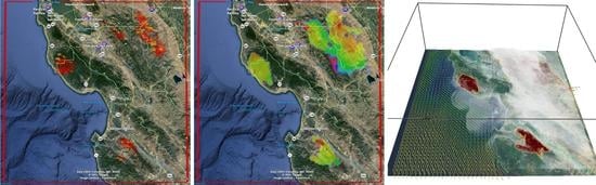
2.1. Study Cases

The summer and fall of 2020 was the most extensive and extreme wildfire season recorded in California history, according to the California Department of Forestry and Fire Protection (CALFIRE) [46]. Many of these fires were started by cloud-to-ground lightning flashes from remnants of Tropical Storm Fausto around August 2020. During this historic fire season, more than 9000 incidents burned over 4 million acres, causing numerous fatalities and damaging or destroying more than 10,000 structures [47]. The abundance, size, and complexity of the fire events make this past wildfire season in California a good testbed for our proposed method. The fire progression histories presented in this paper were processed with the intention of providing fire initialization for subsequent fire modeling studies. The wildfire incidents were filtered by (1) time (2020), (2) space (ONCC and OSCC NIFC GACCs), and (3) burned area (larger than 100 thousand acres), which resulted in the top 10 largest fires of 2020 California wildfire season (Table 1). Figure 1 shows the study domain, along with the location of each wildfire analyzed in this study.

2.2. Satellite Data

For the research, we used satellite Active Fire (AF) products to estimate the progression of wildfires. These products detect thermal anomalies based on the brightness temperature response from spectral bands with wavelengths 4- and 11- μ m. A moving window method characterizes neighboring non-fire background pixels, and fire pixels are further improved using contextual refinement in space and time. The Level-2 (L2) is preferred over the Level-3 (L3) AF products for science use [37]. L2 data is already corrected for cloud and water cover but at the same time maintains important information from the raw products and provides granules with a categorical mask, which classifies every pixel either as missing, clear ground, or fire (Figure 2). On the other hand, L3 data, commonly used operationally and by the public, consists of hotspots only, combined from multiple granules. L3 data is much easier to use and the volume of data is much less, but the distinction between no fire and no data is lost. Finally, in AF data, for every pixel classified as fire, additional information is provided, such as position on the granule, longitude and latitude, fire radiative power, and detection confidence. The last piece of information is essential for the machine learning technique proposed in Section 2.5, since it provides a way to weigh the importance of the data when using a statistical learning method. Unfortunately, unlike fire pixels, clear ground detection pixels are not accompanied by a confidence level. Finally, to process L2 data, one needs to acquire a separate geolocation product, used to define the location of the L2 products from a particular satellite data source. Geolocation of the pixels is defined at their centers.
Moderate Resolution Imaging Spectroradiometer (MODIS) on-board of the Terra and Aqua satellites provides L2 AF products, MOD14 and MYD14 respectively, with four overpasses a day at 1 km resolution [48,49]. In order to geolocate the complete fire mask, geolocation products MOD03 and MYD03 for each satellite [50,51] need to be obtained and associated with every fire mask granule. Visible Infrared Imaging Radiometer Suite (VIIRS) on-board of the Suomi-NPP satellite provide two additional L2 AF products, VNP14 and VNP14IMG, with two overpasses a day at moderate and high spatial resolution (750 m and 375 m), respectively [52,53]. The complete fire mask for these products needs to be geolocated using the VNP03 and VNP03IMG products, respectively [54,55].

2.3. Infrared Fire Perimeters

For large events, National Infrared Operations (NIROPS) provides fire extent data derived from infrared sensors flew on-board aircraft, surveying wildfires, typically at night. These infrared (IR) fire perimeters provide the most accurate representation of the fire front position during the time of the overflight. They are generally accurate at the order of meters, which makes them very useful for situational awareness. However, IR fire perimeters can sometimes be delayed several days after the fire ignition time, and are typically captured at intervals equal to a day or more, assuming that the fire and weather conditions and availability of the resources permit these flights. Although infrared perimeters provide a superior depiction of the spatial fire extent, their temporal frequency is problematic for forecasting applications.
The IR fire perimeters were retrieved from the National Interagency Fire Center (NIFC) Archived Wildfire Perimeters [56] and Wildfire Perimeters [57] databases using ArcGIS API for Python. The perimeter selection was based on the bounding box and time of interest for each incident. Pulling all of the data from both databases ensures that all available IR fire perimeters for each incident are acquired. However, some of these perimeters are duplicated; thus, assessing their acquisition time can be problematic. The databases include three different time definitions: CreateDate, DateCurrent, and PolygonDateTime. Sometimes, inconsistencies exist within this database, likely due to human errors during data entry. The main priority is to use the PolygonDateTime. However, in many cases, this field is not provided. Therefore, the second priority is to use the CreateDate time. Using the CreateDate time may generate inconsistencies where perimeters from different times have the same creation day and time assigned. For those cases, the field DateCurrent is used. To summarize, fire perimeters from the NIFC GIS portal may need manual adjustment, and that each perimeter’s temporal assignment can be quite uncertain.

2.4. Support Vector Machines

The support vector machine (SVM), introduced in Reference [58,59], is a supervised machine learning algorithm. Training an SVM consists of finding a separating surface between two sets of points in a finite dimensional vector space (the training set). The surface, now called a decision surface, is then used to classify other points as belonging to one set or the other, depending on which side of the surface they are.

2.4.1. Linear Separation

In order to solve the separation problem, Vapnik [60] formulated an optimization problem. Consider the two-dimensional example in Figure 3 to explain the idea. Two different sets of points x i , shown as green and red squares, should be separated using a straight line w x + b = 0 , e.g.,  w x i + b > 0 for the red points and w x i + b < 0 for the green points. The same reasoning applies in higher dimension. Suppose we are given column vectors x i R n and labels i = 1 if x i is a red point and i = 1 if x i is a green point. We are looking for w R n and b R such that the sets of red points and the green points are separated by the hyperplane w T x i + b = 0 , i.e.,
w T x i + b > 0 if i = 1 , and w T x i + b < 0 if i = 1 .
Now, scale the coefficients w and b so that w T x i + b 1 for all red points, and w T x i + b 1 for all green points. Then, we can write both inequalities in a common form as i ( w T x i + b ) 1 . Since the distance of the point x and the hyperplane w T x + b = 0 is w x + b / w , the distance of the separating hyperplane from each set is at least 1 / w , and it equals to 1 / w if the equality i ( w T x i + b ) = 1 is attained for at least one point in that set. Thus, the optimal hyperplane w T x + b = 0 that separates the sets and maximizes the distance from each is given by the solution of the quadratic optimization problem
min w , b 1 2 w T w subject to i w T x i + b 1 , i = 1 , , n .
The distance of the hyperplanes w T x + b = 1 and w T x + b = 1 , which equals to d = 2 / w , is called the margin of the separation. The points x i on these hyperplanes are the closest to the separating hyperplane, and they are called support vectors, naming the algorithm after them.

2.4.2. Soft Margins

The constraints i ( w T x i + b ) 1 ensure separation without errors. When the training data cannot be separated without error, one can separate them approximately, minimizing the total error. Thus, we relax the inequalities i ( w T x i + b ) 1 to i ( w T x i + b ) 1 ζ i ,   ζ i > 0 . Geometrically, the point x i is allowed to violate the separation and lie at the distance ζ i / w on the opposite side of the hyperplane. Adding a sum of the violations ζ i with weights C i > 0 to the objective function results in the soft-margin SVM,
min w , b 1 2 w T w + i = 1 n C i ζ i subject to i w T x i + b 1 ζ i , i = 1 , , n .
We will use the weights C i to model the confidence level of the data points ( x i , i ) .

2.4.3. Kernels and Non-Linear Separation

Since linear separation is neither feasible nor desirable in many applications, a kernel technique is used to map the data x i to vectors ϕ ( x i ) in an infinite dimensional vector space, called feature space, where a separating hyperplane is found. Upon mapping back into the input space, the separating hyperplane becomes a non-linear decision surface. The feature space is equipped with an inner product, denoted by · , such that ϕ ( x ) · ϕ ( x ) = K ( x , y ) , where K ( x , y ) is a suitable function, called kernel. In an implementation, vectors in the feature space, its inner product, or the non-linear mapping ϕ , do not need to be used explicitly; rather, the computations are performed on vectors in the input space, with the inner product x T y on replaced by K ( x , y ) . In this work, the kernel is chosen to be a Gaussian radial basis function K ( x i , x j ) = e γ | | x i x j | | 2 . The soft-margin optimization problem (2) in the feature space is
min w , b 1 2 w · w + i = 1 n C i ζ i subject to i w · ϕ ( x i ) + b 1 ζ i . i = 1 , , n .
The solution of (3) is found by solving the dual problem for the vector of Lagrange multipliers α = ( α i ) R n ,
min α 1 2 α T Q α e T α subject to T α = 0 , 0 α i C i , i = 1 , , n ,
where Q i j = i j K ( x i , x j ) is an n × n positive semi-definite matrix, e is the vector of all ones, and  = ( i ) . Once the dual problem (4) is solved, α is found. Then, b is computed from the KKT conditions on Equation (3) as
b = i : 0 < α i < C i y i i f ( α ) | { i | 0 < α i < C i } | , if | i | 0 < α i < C i | > 0 m ( α ) + M ( α ) 2 , otherwise ,
where f ( α ) = 1 2 α T Q α e T α , m ( α ) = min { y i i f ( α ) | α i = 0 , y i = 1 or α i = C i , y i = 1 } , and  M ( α ) = max { y i i f ( α ) | α i = 0 , y i = 1 or α i = C i , y i = 1 } . Then, the decision function is mapped into the input space as
F ( x ) = i = 1 n i α i K ( x i , x ) + b ,
which can be used to classify yet unseen input data x as
( x ) = 1 , if F ( x ) < 0 1 , if F ( x ) 0 .
See Reference [58,59] for more details on the method, and see Reference [61,62] for the specific implementation used.

2.5. Estimation of Fire Arrival Time

2.5.1. Preprocessing

In the initial step, all AF satellite data intersecting the bounding box and time interval of interest are retrieved. The information stored from every clear ground and fire detection pixel includes its latitude, longitude, satellite acquisition time, and confidence level. While clear ground detection pixels do not have a confidence level, they do tend to have higher confidence [36,38]; thus, a sufficient high constant value of 95% is assigned to them (a 100% value can lead to overfitting). All the fire pixels with less than 70% confidence were treated as false alarms and discarded. Every dimension of the data (longitude, latitude, and satellite acquisition time) was then normalized using the min-max feature scaling to have values set between [ 0 , 1 ] . This pre-processing part is critical to avoid the impact of different data ranges on the final solution. The AF satellite data is significantly imbalanced due to a massive amount of clear ground detection pixels. Therefore, a simple under-sampling technique is performed on the clear ground detection pixels. The acquisition and techniques used to pre-process the data as described above can be found in the repository and the code provided in the Supplementary Materials section at the end of the paper.

2.5.2. SVM Deployment

From Section 2.5.1, a three-dimensional training set of points (longitude, latitude, and time) are labeled as ground or fire detection with a confidence level attached to them. The main goal is to find the best separation between these two sets to find the best fire arrival time for any latitude-longitude point in the domain based on these satellite detection data. So, this new approach is not only considering the fire detection pixels but also the clear ground detection pixels, which play an important role, as well. Moreover, the confidence associated with each fire detection contributes to the estimate. Therefore, a generalization of the problem can be defined as a given training set of points x i R p , i = 1 , , n with associated labels i { 1 , 1 } n and confidence levels c i [ 0 , 100 ] . This separation problem can be solved using a machine learning classification method called support vector machine (SVM) described on Section 2.4.
The optimization problem (4) is very sensitive of the value of the parameters C i and γ . Therefore, these optimal hyperparameters need to be tuned so that they capture the properties of the data without over-fitting. These parameters are defined as C i = c i 3 k C , where c i is the confidence level associated with detection x i and k C is a scalar factor; and γ = n k γ p S x , where n is the number of training data points, p = 3 is the dimension of the training data, S x is the population standard deviation of the training data, and k γ is a scalar factor. From these hyperparameters, k C and k γ need to be tuned, since smaller values of k C and k γ , more possibility of over-fitting but less flexibility to follow the data. Therefore, a k-fold cross-validation on an exhaustive grid search on k C and k γ is performed for each experiment using the sklearn.model_selection.GridSearchCV, and k is selected to be 5, which is the most common option. This procedure consists of, for each combination of values k C and k γ , split the training set into k smaller sets and select all combinations between k 1 of these subsets for training purposes and the remaining one subset to validate the results computing the error with independent data. Then, all the errors from the different splits are averaged in order to estimate the final error of prediction for every combination of hyperparameters. Finally, all averaged errors for all combinations of k C and k γ are compared, and the combination of hyperparameters with less error is chosen to retrain the model with all the training data. Since the data is extremely imbalanced, the same proportion of fire and ground detection pixels is maintained in all the splits of the data.
For the purpose of this article, the optimization problem (4) is solved using the python interface with weights for data instances implementation [62] of support vector classification C-SVC from libsvm C++ library [61]. This library is used in the code included in theSupplementary Materials section at the end of the paper.

2.5.3. Postprocessing

Using the SVM method, the L2 AF satellite data from Section 2.2 can be separated using a non-linear hyperplane which can be defined as all the points x such that the decision function is 0, i.e.,  F ( x ) = 0 . However, a unique fire arrival time value at each location is desired and not ensured. As one can observe in Figure 4, a location ( x 1 , x 2 ) can have different temporal values t where F ( x 1 , x 2 , t ) = 0 . Therefore, the fire arrival time at a location ( x 1 , x 2 ) is defined as
T ( x 1 , x 2 ) = min { t R F ( x 1 , x 2 , t ) = 0 } .
However, the existence of such a time t in a location ( x 1 , x 2 ) such that F ( x 1 , x 2 , t ) = 0 is not ensured either. Moreover, the resolution of the volume mesh grid, which the decision function F is evaluated on, can affect the existence of such a time t, as well. Therefore, for all ( x 1 , x 2 ) R 2 , the decision function is approximated using a piecewise polynomial approximation, which is twice continuously differentiable by cubic splines interpolation as
F ( x 1 , x 2 , t ) s ( t ) .
So, interpolate.CubicSpline method of SciPy [63] python package is used to find a piecewise polynomial approximation at each location ( x 1 , x 2 ) . In Figure 4, an example of the piecewise polynomial approximation (blue line) of the vertical profile values of the decision function at a fixed location (orange crosses) is showed. Then, the real roots of this piecewise polynomial approximation can be found easily using roots method of scipy.interpolate.PPoly element as
R x 1 x 2 = { t R s ( t ) = 0 } .
Then, the final definition of the fire arrival time at a location ( x 1 , x 2 ) can be formulated as
T ( x 1 , x 2 ) = M , if R x 1 x 2 = min R x 1 x 2 , otherwise ,
where M is a maximum fire arrival time value associated with a fire arrival time never acquired in the simulation. Finally, one can ensure this maximum value at each location ( x 1 , x 2 ) doing
T ( x 1 , x 2 ) = min ( T ( x 1 , x 2 ) , M ) .
Figure 4 shows an example of the three roots of the piecewise polynomial approximation of the vertical profile values of the decision function at a fixed location (green circles) and the minimum t root of the same approximation (red circle). This minimum t is what will be defined as the fire arrival time at this fixed location. This process is repeated for each point in the domain. The fire arrival time estimation described in this section is part of the python code included in the Supplementary Materials section at the end of the paper.
Finally, the results are transformed back to original scales using the same scale parameters as were used in the pre-processing in Section 2.5.1.

3. Results

The fire arrival time estimation using the machine learning method from satellite data described in Section 2 is applied to the top 10 largest wildfires in California this past fire season 2020 (Table 1). The evaluation of the results is focused on two main analyses (1) L2 AF satellite data assessment to identify where the spatial resolution and temporal frequency from satellite detection pixels could impact the SVM estimation, and (2) the validation of fire arrival time estimation where the resulting fire arrival time is compared to IR observed fire perimeters considering two commonly used metrics: area burned and spatial discrepancy.

3.1. L2 AF Satellite Data Assessment

L2 AF satellite data is compared to IR fire perimeters in order to assess the spatiotemporal correlation between the IR fire perimeters and the fire detection pixels. For every IR fire perimeter, the fire pixels detected between the previous and the current perimeter times are identified. Then, the percentage of fire detection pixels falling spatially between the IR perimeters is calculated. Figure 5 shows an example of that computation for the August Complex between 2 September and 15 September 2020. The blue and green filled areas represent the observed IR fire perimeters, and scatter empty circles are L2 AF fire detection pixels sensed between perimeter times. The green circles show detection pixels falling spatially inside the two consecutive perimeters, and the red ones otherwise. The fire detection pixels falling inside the earliest perimeter could be associated to some smoldering happening at those locations so they are not considered to be a satellite error. The percentage of the green circles or fire detection pixels between the perimeters estimates the spatiotemporal correlation between L2 AF fire detection pixels and IR fire perimeters. When the earliest IR perimeter is considered, the fire detection pixels are filtered, and the percentage is calculated from the start of the fire event as specified in Table 1.
The variability of the percentages varies among analyzed cases. The fewer IR perimeters, the larger percentage because more fire detection pixels are likely to fall in between the perimeters. For instance, the LNU Complex (LNU) has percentages all >80% with 91% average, while the Red Salmon Complex (RSC) has most of the percentages <70% with 69% average. In addition, for the same reason, the less spaced out in time the IR perimeters are, the smaller the correlations were between the satellite data and airborne perimeters (smaller percentages). Finally, we can observe that all the transparent circles happened at the beginning or the end of the fire event (LNU, SD, and RSC). Sometimes, at the beginning of the fire, IR fire perimeters are captured before the fire is big enough to be sensed by the AF satellite data. Moreover, at the end of the fire, when the intensity of the fire is very low, the satellites are not capable of detecting fire detection pixels.
Percentages on the first row of Table 2 shows how almost all the cases have a percentage larger than 70%, and a total average of 81%. Therefore, the fire detection pixels are mostly correlated to the IR fire perimeters, indicating a good opportunity to predict the fire evolution from this source of data. Simultaneously, these results proves the necessity of using a method that considers implicit errors in the data since we have an error on every 2 out of 10 pixels. We believe the major source in this analysis of error comes from the temporal misspecification of IR perimeters. Errors in satellite fire detection pixels are likely due to relatively low spatial resolution and large spatial inhomogeneity, which make it difficult for processing algorithms to separate the hot spots from the background. In addition, satellite data can have geolocation errors caused by the fact that every pixel’s location is defined to be a point at the center of the pixel, which is a crude assumption.

3.2. Evaluation of the Fire Arrival Time Estimation

As described in Section 2.5.3, the fire progression is parameterized as a fire arrival time, which is a real-valued function defining for each location x R 2 the time that the fire arrives at that location T ( x ) . Note that by defining the fire progression in such a way, fire perimeters can be constructed at any temporal interval by computing contours at different times. For evaluations utilizing observed IR fire perimeters, hourly contours are computed from the fire arrival times estimated by the machine learning technique for the 10 largest wildfires in California during the summer of 2020. The evaluation is performed at IR perimeter times using two common metrics: burned area and spatial discrepancies.

3.2.1. Burned Area

For each hourly contour, the burned area is computed and plotted as solid blue lines in Figure 6. These results can then be compared to burned area estimates from observed IR fire perimeters represented as colored circles. In most cases, the colored circles lie close to the blue lines indicating good agreement between observed IR fire perimeters and resulting fire arrival time from the proposed machine learning method. For each fire, the mean absolute percentage error between the burned area from the SVM method and IR fire perimeters is calculated to quantify their agreement, showing values between 3–20%, with an average of 12% (Table 2). In addition, most of the increases in burned area are represented by the fire arrival time estimation. However, the burned area from SVM estimation tends to overestimate relative to the observed IR fire perimeters. For each fire, the mean percentage of overprediction on the errors (Table 2) is calculated as the area overpredicted over the area wrongly classified (expressed on percentage), showing that, on average, 63% of the area burned wrongly estimated by the SVM method is by overprediction. In fact, the only case that underestimated more than overestimated is the Slater/Devil (SD) wildfire. This result is caused by the fact that, in the SVM estimation, the fire and clear ground pixels are integrated as spatiotemporal points located at the pixel center. However, the algorithm classifies pixels using the whole extent of the pixel, which can be more than 1 km 2 depending on the scan angle and product resolution. For future work, a non-convex optimization could be applied to overcome this limitation. Furthermore, as one can observe in the results from Slater/Devil (SD) and LNU Lightning Complex (LNU) wildfires, the machine learning method can successfully estimate burnt area during the initial stage of fire progression before satellite fire detection pixels by interpolating between the clear ground detection pixels and the earliest fire detection pixels. In both cases, the IR fire perimeter circles are transparent, indicating the absence of fire detection pixels prior to the perimeter time. Before the first fire detection pixel, the clear ground detection pixels inform where the fire is not burning to the machine learning method, allowing the capture of fire progression prior to the appearance of fire detection pixels. In general, final burned areas estimated from the SVM method are also very close to the final burned areas reported for each fire in Table 1. Table 2 reports, for each fire, the percentage error between total burned areas from the machine learning method and reported by CALFIRE showing total burned areas overestimated by the SVM method in positive values (AC, LNU, CK, NC, SQF, DC, and BC) and underestimated in negative values (SCU, SD, and RSC). The percentage errors are between −2% and 13%, with an absolute average of 5% for all the fires.

3.2.2. Spatial Discrepancies

For each top 10 wildfires, spatial discrepancies at every observed IR fire perimeter time are computed. In this work, we estimate spatial discrepancies using the Sørensen’s coefficient (SC) [64], calculated as:
SC = 2 A 2 A + B + C ,
where A is the area burned for both IR and SVM estimated perimeters representing matches (true positives), B is the area burned by IR perimeter and unburned by SVM (false negatives), and C is the area indicated as burned by SVM estimated perimeter and unburned by IR perimeter (false positives). So, in other words, A is the area burned with an agreement between both perimeters, B the area burned underpredicted by the SVM method, and C the area burned overpredicted by the SVM method. SC ranges between 0 and 1, where values close to 1 represent a high spatial agreement between the observed IR perimeter and the SVM estimated one. Figure 7 shows an example of how the SC can be computed for the August Complex fire on 15 September 2020. The spatial discrepancy between an IR perimeter (discontinuous blue polygon) and an SVM estimated perimeter (discontinuous red polygon) is computed using burned areas A (green area), B (blue area), and C (red area). The SC value for this example is 0.915, proving a high spatial agreement between both perimeters.
Two other scalar attributes for characterizing the contingency table of SVM versus IR perimeters [65] are the Probability of Detection (POD) and the False Alarm Ratio (FAR), calculated as
POD = A A + B and FAR = C A + C ,
which range between 0 and 1. The POD, commonly known as the hit rate or sensitivity, is the ratio of fire burned area predicted using the SVM method that is also burned by the IR fire perimeters. Therefore, values close to 1 indicate that the SVM method detects where the fire is happening effectively. The FAR is the ratio of fire burned area predicted using the SVM method that is not burned by the IR fire perimeters. It has a negative orientation; values close to 0 indicate that the SVM method is not burning erroneous regions.
Table 2 shows for each fire, the POD, FAR, and SC averaged at all the times that IR fire perimeters were provided. All the mean POD values are greater than 0.8, except for LNU. The value of 0.68 in the LNU fire is caused by the fact that only three IR fire perimeters were provided, and the first of those was measured before any fire detection pixel was sensed (Figure 6). However, an average POD value of 0.86 indicates that if the SVM method characterizes a location as having fire, the IR perimeters also indicate fire 86% of the time. All the mean FAR values are around 0.2 with the same previous exception of LNU because of the same reason. An average FAR value of 0.21 indicates that, 21% of the time, SVM is predicting fire where IR perimeters show none. Appendix A provides a more extensive analysis of POD and FAR values and their relation to the SVM overprediction of the fire extent. Finally, all the mean SC values are around 0.8 with the same previous exception of LNU because of the same reason. The average for all the wildfires is 0.82, proving that the SVM method can provide an accurate spatial representation of the fire extent.
Figure 8 depicts the SC (black line with dots) for the top 10 largest wildfires of 2020 in California at every IR fire perimeter time. The dashed black vertical line represents the time of the August Complex (AC) wildfire snapshot showed in Figure 5 and Figure 7. Overall, SC values are close to 1, indicating a high spatial agreement between the fire extent estimated by SVM and derived from IR fire perimeters. The SC tends to increase over time as it is gradually easier for the SVM method (based on relatively coarse satellite data) to accurately capture the fire area as the number of fire detection pixels increases. Consequently, some of the lowest agreement values occur at the time of the first IR fire perimeter when the number of fire pixels is low due to the small fire extent (see initial fire burned areas for LNU, RSC, and BC fires in Figure 6). Furthermore, in Red Salmon Complex (RSC) fire, there are sudden and abrupt changes in the SC value. These fluctuations are caused by the abundance of observed IR fire perimeters for this particular case, which provided very frequent fire perimeter scans.
To better understand the observed SC variability, the matching area A (dotted green line), false-negative area B (dotted blue line), and false-positive area C (dotted red line) are plotted in the same Figure 8. Plotting these areas allows us to identify the impact of over and under-prediction on the SC values. For instance, as mentioned in the previous section, the SVM method tends to overestimate burned area as the dotted red lines are generally over the dotted blue lines. In fact, on average, the dotted red lines are over the dotted blue lines by 63% (Table 2). In addition, the increases in the under and overpredicted areas are generally associated with significant fire growth as indicated by the corresponding increases in the intersecting areas (dotted green lines), which can be used as a proxy for the fire size.
Figure 9 shows a comparison between L2 AF fire detection pixels, results from SVM estimation, and observed IR fire perimeters for five special cases out of the top 10 largest wildfires of 2020 in California, one per row. This figure allows for a visual assessment of spatial discrepancies. All the plots are colored using a rainbow colormap with the range depending on the event start and end times from Table 1. The first column shows a scatter plot of the L2 AF fire detection pixels plotted in different sizes depending on their confidence level, the second column depicts the continuous fire arrival time from the machine learning method, the third column plots the same previous fire arrival time but only at the IR perimeter times, and the fourth column shows the observed IR fire perimeters. The rest of the 10 cases can be found in Appendix B.
The first two columns of Figure 9 visualize how the SVM method integrates the satellite data into a continuous fire progression. For instance, looking at the August Complex (AC) and SCU Lightning Complex (SCU) wildfires (Figure 9a–h), it can be seen that this method ignores fire detection pixels of low confidence level (red circles) while preserving small fires for cases where the confidence level of those detection pixels are high (green circles). The two isolated dark blue detection pixels in the north-center and center-west surrounded by a red circle in Figure 9a are filtered out and are not present in the SVM results shown in the next column (Figure 9b). However, at the same time, the SVM still preserves small fires, like the south-west cyan one (surrounded by a green circle in Figure 9a), as long as the confidence of the detection pixels is high. A closer examination of the fire detection pixels in this region revealed that these pixels correspond to the much smaller Oak fire that was not mapped by NIROPS focused on the August Complex fire. A similar situation happens with the SCU wildfire, where the method is able to distinguish a much smaller fire not mapped by NIROPS, the Coyote fire (detection pixels surrounded by a green circle in Figure 9e).
The last two columns illustrate spatial discrepancies between SVM-estimated and observed fire extent at the time of IR perimeters. While the level of details provided by the SVM method is not as high as in the IR perimeters in terms of spatial representation, the SVM method does still provided a very good representation of the overall fire progression. Since the SVM method is based on satellite detection pixels, it is particularly valuable in situations where the number of available IR perimeters is low (SCU, LNU, and SD) or non-existent. For these cases, the method proposed in this article provides a continuous near-real-time representation of the fire progression not available from other data sources.
To summarize, the SVM method proposed here is sometimes sensitive to false alarms from the L2 AF satellite data. For instance, in the DC wildfire (Figure 9q–t), false positive detection pixels over the ocean resulted in unrealistic offshore fire progression. This problem could be potentially rectified by increasing the threshold of the confidence level below which fire detection pixels are filtered out or use ancillary data to generate a mask correcting false positive detection pixels over nonburnable areas corresponding to water bodies. The LNU wildfire (Figure 9i–l) is a good example illustrating that the proposed method can estimate the fire progression of three concurrent fires. However, the accuracy of the method may be limited by sparse fire detection pixels. The white holes produced at the start of the SD wildfire illustrates this problem (Figure 9m–p). A higher spatiotemporal resolution in the L2 AF satellite data or/and further refinement of the method would be required to overcome this problem.

4. Discussion and Conclusions

The proposed SVM method integrates MODIS and VIIRS active fire data to estimate fire progression using a machine learning method. Both datasets are provided by polar-orbiting satellites and deliver global coverage. Therefore, the presented method can be applied globally. The method incorporates both fire and clear ground detection pixels in a spatiotemporal space and can integrate additional data to overcome potential problems associated with limited temporal and spatial resolutions of the current satellite products. For instance, while, in this study, the airborne IR fire perimeters were used for validation only, the method can also integrate both the satellite data and airborne IR observations for improved accuracy.
In lieu of a typical spatial interpolation, the presented SVM method identifies fires spatiotemporally, integrating fire and clear ground detection pixels using the fire arrival time concept. The fire arrival time is calculated as the minimal time separating areas burning and not burning by using a cubic splines interpolation at each location. The satellite observations, which are discrete in time, are used to train the machine learning method presented here, which provides a continuous description of the fire progression. The fire extent can then be estimated at any given time in contrast with the similar studies mentioned in the introduction, which are designed to provide a daily estimate of the fire extent given the satellite data. Moreover, this novel method was proven to deal with false alarms or outliers by utilizing the confidence level associated with each fire detection pixel. The method also handles better small-scale irregularities since it provides a smooth estimation of the fire evolution for its kernel mathematical properties. Finally, the proposed method provides good quality estimates between satellite overpasses since it uses a weighted learning process not only utilizing the fire detection pixels but also the clear ground ones.
Even though, on average, 81% of the L2 AF fire detection pixels were spatiotemporally correlated to the observed IR fire perimeters, the need for a statistical learning method was proven to limit the overfitting of the data. The method presented deals with that by utilizing the confidence levels provided with satellite fire detection pixels. This strategy allows the fire progression to be primarily driven by high-confidence fire detection pixels, while low-confidence pixels are filtered out, thus having a limited impact on the estimated fire progression. This feature allows this method to deliver robust results even when the input satellite data suffer from errors associated with obstructions of satellite view by dense smoke or clouds, oblique scan angles, terrain shading, or other factors, without compromising the representation of small fires.
The resulting SVM-based fire arrival time estimates were evaluated using independent observed IR fire perimeters for 10 different fires. Both the time progression of the burned area and the spatial fire extent at the perimeter times matched well IR observations proving the method’s ability to provide a continuous near-real-time estimation of the fire progression not available from other data sources. On average, 12% mean absolute percentage error of burned area, 5% percentage error of total burned area, 0.21 False Alarm Ratio, 0.86 Probability of Detection, and 0.82 Sørensen’s coefficient indicated a high spatiotemporal agreement between estimated fire arrival time and airborne IR perimeters.
The SVM method does have some limitations that should be considered. The SVM method generally tended to overestimate the fire area. On average, 63% of the errors between the SVM method and IR fire perimeters are caused by an overestimation. This problem is believed to be associated with the fact that fire and clear ground detection pixels are integrated as spatiotemporal points located at the pixel center. However, the detection algorithm classifies pixels using the whole extend of the pixel, which can be much larger than one square kilometer, especially for oblique scan angles. Therefore, for future work, we propose to deploy a non-convex optimization to overcome this limitation. In addition, the SC representing the level of agreement between the SVM and IR derived perimeters tends to be lower at the beginning of the fire events, when the number of satellite detection pixels was low and when the size of the fire was small. We believe that future data sources with higher spatial and temporal resolutions may alleviate this problem. Future work could also include a systematic study focused on better representation of the confidence threshold used to filter out false fire detection pixels, as well as exploration of more meaningful ways to tune hyperparameters. The method could also benefit from the use of ancillary data allowing to avoid false fire detection pixels over unburnable regions, as well as incorporating other satellite data sources, like GOES or burn scar data, among others.

Supplementary Materials

The Python code acquiring L2 AF satellite data intersecting an AOI and a time interval as mentioned on Section 2.2, running the SVM method described on Section 2.4, and estimating fire arrival time as proposed on Section 2.5.3 is available online at https://github.com/openwfm/JPSSdata (accessed on 1 June 2021).

Author Contributions

Conceptualization, A.F. and J.M.; methodology, A.F., J.M., and J.H.; mathematics, J.M.; software and visualization, A.F.; supervision and coordination, J.M.; selection of case studies and evaluation of results, D.V.M., A.K., and K.H.; writing–original draft preparation, A.F.; writing–review and editing, all coauthors; project administration, K.H.; funding acquisition, K.H., A.K., and J.M. All authors have read and agreed to the published version of the manuscript.

Funding

This project was funded by the NASA Applied Sciences Program grant 80NSSC19K1091 and National Science Foundation grant ICER-1664175.

Institutional Review Board Statement

Not applicable.

Informed Consent Statement

Not applicable.

Data Availability Statement

Not applicable.

Acknowledgments

The authors would like to acknowledge high-performance computing support from Cheyenne (doi:10.5065/D6RX99HX) provided by NCAR’s Computational and Information Systems Laboratory, sponsored by the National Science Foundation. The computing support from the Center for High Performance Computing (University of Utah) and Center for Computational Mathematics (University of Colorado Denver) is greatly appreciated.

Conflicts of Interest

The authors declare no conflict of interest.

Abbreviations

The following abbreviations are used in this manuscript:
WRFWeather Research and Forecasting
CALFIRECalifornia Department of Forestry and Fire Protection
ONCCNorthern California Geographic Area Coordination Center
OSCCSouthern California Geographic Area Coordination Center
NIROPSNational Infrared Operations
GACCGeographic Area Coordination Centers
AOIArea Of Interest
L2Level-2
AFActive Fire
MODISModerate Resolution Imaging Spectroradiometer
VIIRSVisible Infrared Imaging Radiometer Suite
GOESGeostationary Operational Environmental Satellite
NIFCNational Interagency Fire Center
MLMachine Learning
SVMSupport Vector Machine
SCSørensen’s coefficient
PODProbability of Detection
FARFalse Alarm Ratio

Appendix A. Performance Analysis

To further assess the performance of the SVM method using IR fire perimeters, this appendix includes a more concise analysis of some metrics averaged and shown in Table 2, Probability of Detection (POD) and False Alarm Ratio (FAR). These metrics were initially described and analyzed in Section 3.2.2. For every fire and at every IR fire perimeter time, we computed A or the area burned for both IR and SVM (true positives), B or the area burned by IR and unburned by SVM (false negatives), and C or the area burned by SVM and unburned by IR (false positives). These three parameters computed at every fire and IR fire perimeter time are then used to compute POD and FAR using equations in (5). Figure A1 plots every case as a function of 1-FAR or success ratio on the independent axis and POD on the dependent axis using a 2D scatter plot colored by the wildfire. This kind of plot is commonly called performance diagram [65] and provides another way to analyze differences between perimeters extracted from the SVM method and the observed IR fire perimeters. The plot shows two new metrics, the critical success index using black dashed curves and the bias represented as gray dotted lines. The critical success index is the proportion of area correctly burned (value between 0 and 1) and represents the accuracy of the SVM method. The bias is the ratio of area burned estimated by SVM over the area burned by the IR fire perimeters. Therefore, a bias of 1 indicates that the SVM method is unbiased with respect to IR fire perimeters. The SVM method overestimates the fire extent if the bias is greater than 1 and underestimating if less than 1.
Figure A1. Performance diagram of the top 10 largest wildfires of 2020 in California (Table 1). Each colored star depicts the performance of the SVM method compared to the IR fire perimeters at one specific IR fire perimeter time. The color of the star indicates the wildfire case. The black dashed curves are critical success index, and the gray dotted lines are bias.
Remotesensing 13 02203 g0a1
The first thing that one can notice in Figure A1 is the red outlier. This point corresponds to the first perimeter of the LNU fire, which was emphasized in Section 3.2.2 to be a problem due to the fact that the IR fire perimeter was measured prior to any fire detection pixel. In addition, one can observe that most of the points have a bias slightly greater than 1 proving the SVM overprediction of the fire extent observed in Section 3.2.2. However, there is one pink point clearly underpredicting the fire extent which corresponds to the first perimeter of the SD fire, which was shown in Table 2 to be the only case which SVM underpredicted more than overpredicted with MP Overpredicted of 44%. Finally, one can observe that most of the points have a critical success index close to 1 proving that the SVM method can provide accurate fire arrival times for improving fire modeling.

Appendix B. Rest of the Cases

For reference, Figure A2 in this appendix includes all the cases missing in Figure 9.
Figure A2. The rest of the cases (one per row) from the top 10 largest wildfires of 2020 in California (Table 1). L2 AF satellite fire detection pixels (first column), continuous fire arrival time from SVM (second column), perimeters from SVM at IR perimeters time (third column), and observed IR fire perimeters (fourth column).
Remotesensing 13 02203 g0a2

References

  1. Westerling, A.L. Warming and Earlier Spring Increase Western U.S. Forest Wildfire Activity. Science 2006, 313, 940–943. [Google Scholar] [CrossRef] [PubMed] [Green Version]
  2. Liu, Y.; Stanturf, J.; Goodrick, S. Trends in global wildfire potential in a changing climate. For. Ecol. Manag. 2010, 259, 685–697. [Google Scholar] [CrossRef]
  3. Dennison, P.E.; Brewer, S.C.; Arnold, J.D.; Moritz, M.A. Large wildfire trends in the western United States, 1984–2011. Geophys. Res. Lett. 2014, 41, 2928–2933. [Google Scholar] [CrossRef]
  4. Abatzoglou, J.T.; Williams, A.P. Impact of anthropogenic climate change on wildfire across western US forests. Proc. Natl. Acad. Sci. USA 2016, 113, 11770–11775. [Google Scholar] [CrossRef] [Green Version]
  5. Jaffe, D.; Hafner, W.; Chand, D.; Westerling, A.; Spracklen, D. Interannual Variations in PM2.5 due to Wildfires in the Western United States. Environ. Sci. Technol. 2008, 42, 2812–2818. [Google Scholar] [CrossRef] [PubMed]
  6. Anderson, J.O.; Thundiyil, J.G.; Stolbach, A. Clearing the Air: A Review of the Effects of Particulate Matter Air Pollution on Human Health. J. Med. Toxicol. 2011, 8, 166–175. [Google Scholar] [CrossRef] [PubMed] [Green Version]
  7. Kim, K.H.; Kabir, E.; Kabir, S. A review on the human health impact of airborne particulate matter. Environ. Int. 2015, 74, 136–143. [Google Scholar] [CrossRef] [PubMed]
  8. Mallia, D.V.; Lin, J.C.; Urbanski, S.; Ehleringer, J.; Nehrkorn, T. Impacts of upwind wildfire emissions on CO, CO2, and PM2.5 concentrations in Salt Lake City, Utah. J. Geophys. Res. Atmos. 2015, 120, 147–166. [Google Scholar] [CrossRef]
  9. Spracklen, D.V.; Mickley, L.J.; Logan, J.A.; Hudman, R.C.; Yevich, R.; Flannigan, M.D.; Westerling, A.L. Impacts of climate change from 2000 to 2050 on wildfire activity and carbonaceous aerosol concentrations in the western United States. J. Geophys. Res. 2009, 114. [Google Scholar] [CrossRef]
  10. Clark, T.L.; Jenkins, M.A.; Coen, J.; Packham, D. A Coupled Atmosphere-Fire Model: Convective Feedback on Fire-Line Dynamics. J. Appl. Meteorol. 1996, 35, 875–901. [Google Scholar] [CrossRef] [Green Version]
  11. Clark, T.; Jenkins, M.; Coen, J.; Packham, D. A Coupled Atmosphere-Fire Model: Role of the Convective Froude Number and Dynamic Fingering at the Fireline. Int. J. Wildland Fire 1996, 6, 177. [Google Scholar] [CrossRef] [Green Version]
  12. Coen, J.; Schroeder, W.; Quayle, B. The Generation and Forecast of Extreme Winds during the Origin and Progression of the 2017 Tubbs Fire. Atmosphere 2018, 9, 462. [Google Scholar] [CrossRef] [Green Version]
  13. Peace, M.; Mattner, T.; Mills, G.; Kepert, J.; McCaw, L. Fire-Modified Meteorology in a Coupled Fire–Atmosphere Model. J. Appl. Meteorol. Climatol. 2015, 54, 704–720. [Google Scholar] [CrossRef]
  14. Clark, T.L.; Radke, L.; Coen, J.; Middleton, D. Analysis of Small-Scale Convective Dynamics in a Crown Fire Using Infrared Video Camera Imagery. J. Appl. Meteorol. 1999, 38, 1401–1420. [Google Scholar] [CrossRef] [Green Version]
  15. Coen, J.; Mahalingam, S.; Daily, J. Infrared Imagery of Crown-Fire Dynamics during FROSTFIRE. J. Appl. Meteorol. 2004, 43, 1241–1259. [Google Scholar] [CrossRef] [Green Version]
  16. Clements, C.B.; Zhong, S.; Goodrick, S.; Li, J.; Potter, B.E.; Bian, X.; Heilman, W.E.; Charney, J.J.; Perna, R.; Jang, M.; et al. Observing the Dynamics of Wildland Grass Fires: FireFlux—A Field Validation Experiment. Bull. Am. Meteorol. Soc. 2007, 88, 1369–1382. [Google Scholar] [CrossRef] [Green Version]
  17. Lareau, N.P.; Clements, C.B. The Mean and Turbulent Properties of a Wildfire Convective Plume. J. Appl. Meteorol. Climatol. 2017, 56, 2289–2299. [Google Scholar] [CrossRef]
  18. Lareau, N.P.; Nauslar, N.J.; Abatzoglou, J.T. The Carr Fire Vortex: A Case of Pyrotornadogenesis? Geophys. Res. Lett. 2018, 45, 13107–13115. [Google Scholar] [CrossRef]
  19. Clark, T.L.; Coen, J.; Latham, D. Description of a Coupled Atmosphere-Fire Model. Int. J. Wildland Fire 2004, 13, 49–64. [Google Scholar] [CrossRef] [Green Version]
  20. Mandel, J.; Beezley, J.D.; Coen, J.L.; Kim, M. Data Assimilation for Wildland Fires: Ensemble Kalman filters in coupled atmosphere-surface models. IEEE Control Syst. Mag. 2009, 29, 47–65. [Google Scholar] [CrossRef] [Green Version]
  21. Mandel, J.; Beezley, J.D.; Kochanski, A.K. Coupled atmosphere-wildland fire modeling with WRF 3.3 and SFIRE 2011. Geosci. Model Dev. 2011, 4, 591–610. [Google Scholar] [CrossRef] [Green Version]
  22. Filippi, J.B.; Bosseur, F.; Pialat, X.; Santoni, P.A.; Strada, S.; Mari, C. Simulation of Coupled Fire/Atmosphere Interaction with the MesoNH-ForeFire Models. J. Combust. 2011, 2011, 1–13. [Google Scholar] [CrossRef] [Green Version]
  23. Coen, J. Modeling wildland fires: A description of the Coupled Atmosphere-Wildland Fire Environment model (CAWFE); NCAR/TN-500+STR; NCAR: Boulder, CO, USA, 2013. [Google Scholar] [CrossRef]
  24. Kochanski, A.; Jenkins, M.; Mandel, J.; Beezley, J.; Krueger, S. Real time simulation of 2007 Santa Ana fires. For. Ecol. Manag. 2013, 294, 136–149. [Google Scholar] [CrossRef] [Green Version]
  25. Mandel, J.; Amram, S.; Beezley, J.D.; Kelman, G.; Kochanski, A.K.; Kondratenko, V.Y.; Lynn, B.H.; Regev, B.; Vejmelka, M. Recent advances and applications of WRF-SFIRE. Nat. Hazards Earth Syst. Sci. 2014, 14, 2829–2845. [Google Scholar] [CrossRef] [Green Version]
  26. Jiménez, P.; Muñoz-Esparza, D.; Kosović, B. A High Resolution Coupled Fire–Atmosphere Forecasting System to Minimize the Impacts of Wildland Fires: Applications to the Chimney Tops II Wildland Event. Atmosphere 2018, 9, 197. [Google Scholar] [CrossRef] [Green Version]
  27. Giannaros, T.M.; Lagouvardos, K.; Kotroni, V. Performance Evaluation of an Operational Rapid Response Fire Spread Forecasting System in the Southeast Mediterranean (Greece). Atmosphere 2020, 11, 1264. [Google Scholar] [CrossRef]
  28. Sethian, J.A. A fast marching level set method for monotonically advancing fronts. Proc. Nat. Acad. Sci. USA 1996, 93, 1591–1595. [Google Scholar] [CrossRef] [PubMed] [Green Version]
  29. Finney, M.A. Fire growth using minimum travel time methods. Can. J. For. Res. 2002, 32, 1420–1424. [Google Scholar] [CrossRef]
  30. Mandel, J.; Beezley, J.D.; Kochanski, A.K.; Kondratenko, V.Y.; Kim, M. Assimilation of Perimeter Data and Coupling with Fuel Moisture in a Wildland Fire–Atmosphere DDDAS. Procedia Comput. Sci. 2012, 9, 1100–1109. [Google Scholar] [CrossRef] [Green Version]
  31. Kochanski, A.K.; Mallia, D.V.; Fearon, M.G.; Mandel, J.; Souri, A.H.; Brown, T. Modeling Wildfire Smoke Feedback Mechanisms Using a Coupled Fire-Atmosphere Model With a Radiatively Active Aerosol Scheme. J. Geophys. Res. Atmos. 2019, 124, 9099–9116. [Google Scholar] [CrossRef]
  32. Mallia, D.V.; Kochanski, A.K.; Kelly, K.E.; Whitaker, R.; Xing, W.; Mitchell, L.E.; Jacques, A.; Farguell, A.; Mandel, J.; Gaillardon, P.E.; et al. Evaluating Wildfire Smoke Transport Within a Coupled Fire-Atmosphere Model Using a High-Density Observation Network for an Episodic Smoke Event Along Utah’s Wasatch Front. J. Geophys. Res. Atmos. 2020, 125. [Google Scholar] [CrossRef]
  33. Mandel, J.; Kochanski, A.K.; Vejmelka, M.; Beezley, J.D. Data Assimilation of Satellite Fire Detection in Coupled Atmosphere-Fire Simulations by WRF-SFIRE. In Advances in Forest Fire Research; Viegas, D.X., Ed.; Coimbra University Press: Coimbra, Portugal, 2014; pp. 716–724. [Google Scholar] [CrossRef] [Green Version]
  34. Farguell Caus, A.; Haley, J.; Kochanski, A.K.; Fité, A.C.; Mandel, J. Assimilation of Fire Perimeters and Satellite Detections by Minimization of the Residual in a Fire Spread Model. In Computational Science—ICCS 2018; Shi, Y., Fu, H., Tian, Y., Krzhizhanovskaya, V.V., Lees, M.H., Dongarra, J., Sloot, P.M.A., Eds.; Springer International Publishing: Cham, Switzerland, 2018; pp. 711–723. [Google Scholar] [CrossRef] [Green Version]
  35. Mandel, J.; Kochanski, A.K.; Ellicot, E.A.; Haley, J.; Hearn, L.; Farguell, A.; Hilburn, K. Retrieving Fire Perimeters and Ignition Points of Large Wildfires from Satellite Observations. In Proceedings of the Poster NH23C 0859, AGU Fall Meeting, Washington DC, USA, 10–14 December 2018. [Google Scholar] [CrossRef] [Green Version]
  36. Giglio, L.; Schroeder, W.; Justice, C.O. The collection 6 MODIS active fire detection algorithm and fire products. Remote Sens. Environ. 2016, 178, 31–41. [Google Scholar] [CrossRef] [PubMed] [Green Version]
  37. Giglio, L.; Schroeder, W.; Hall, J.V.; Justice, C.O. MODIS Collection 6 Active Fire Product User’s Guide Version 2.6. Department of Geographical Sciences, University of Maryland. 2020. Available online: https://modis-fire.umd.edu/files/MODIS_C6_Fire_User_Guide_C.pdf (accessed on 7 March 2021).
  38. Schroeder, W.; Giglio, L. Visible Infrared Imaging Radiometer Suite (VIIRS) 375 m Active Fire Detection and Characterization Algorithm Theoretical Basis Document 1.0. 2016. Available online: https://viirsland.gsfc.nasa.gov/PDF/VIIRS_activefire_375m_ATBD.pdf (accessed on 28 August 2018).
  39. Schmit, T.J.; Griffith, P.; Gunshor, M.M.; Daniels, J.M.; Goodman, S.J.; Lebair, W.J. A Closer Look at the ABI on the GOES-R Series. Bull. Am. Meteorol. Soc. 2017, 98, 681–698. [Google Scholar] [CrossRef]
  40. Mu, M.; Randerson, J.T.; van der Werf, G.R.; Giglio, L.; Kasibhatla, P.; Morton, D.; Collatz, G.J.; DeFries, R.S.; Hyer, E.J.; Prins, E.M.; et al. Daily and 3-hourly variability in global fire emissions and consequences for atmospheric model predictions of carbon monoxide. J. Geophys. Res. Atmos. 2011, 116. [Google Scholar] [CrossRef]
  41. Schroeder, W.; Prins, E.; Giglio, L.; Csiszar, I.; Schmidt, C.; Morisette, J.; Morton, D. Validation of GOES and MODIS active fire detection products using ASTER and ETM+ data. Remote Sens. Environ. 2008, 112, 2711–2726. [Google Scholar] [CrossRef]
  42. Fusco, E.J.; Finn, J.T.; Abatzoglou, J.T.; Balch, J.K.; Dadashi, S.; Bradley, B.A. Detection rates and biases of fire observations from MODIS and agency reports in the conterminous United States. Remote Sens. Environ. 2019, 220, 30–40. [Google Scholar] [CrossRef]
  43. Veraverbeke, S.; Sedano, F.; Hook, S.J.; Randerson, J.T.; Jin, Y.; Rogers, B.M. Mapping the daily progression of large wildland fires using MODIS active fire data. Int. J. Wildland Fire 2014, 23, 655. [Google Scholar] [CrossRef] [Green Version]
  44. Scaduto, E.; Chen, B.; Jin, Y. Satellite-Based Fire Progression Mapping: A Comprehensive Assessment for Large Fires in Northern California. IEEE J. Sel. Top. Appl. Earth Obs. Remote Sens. 2020, 13, 5102–5114. [Google Scholar] [CrossRef]
  45. Parks, S.A. Mapping day-of-burning with coarse-resolution satellite fire-detection data. Int. J. Wildland Fire 2014, 23, 215. [Google Scholar] [CrossRef]
  46. Yan, H.; Mossberg, C.; Moshtaghian, A.; Vercammen, P. California Sets New Record for Land Torched by Wildfires as 224 People Escape by Air from a ’Hellish’ Inferno. 2020. Available online: https://www.cnn.com/2020/09/05/us/california-mammoth-pool-reservoir-camp-fire/index.html (accessed on 10 December 2020).
  47. California Department of Forestry and Fire Protection (CALFIRE). 2020 Incident Archive. 2020. Available online: https://www.fire.ca.gov/incidents/2020 (accessed on 10 December 2020).
  48. Giglio, L.; Justice, C. MODIS/Terra Thermal Anomalies/Fire 5-Min L2 Swath 1 km V061; 2020. [Google Scholar] [CrossRef]
  49. Giglio, L.; Justice, C. MODIS/Aqua Thermal Anomalies/Fire 5-Min L2 Swath 1 km V061; 2020. [Google Scholar] [CrossRef]
  50. MODIS Science Data Support Team. MODIS/Terra Geolocation Fields 5-Min L1A Swath 1 km; 2017. [Google Scholar] [CrossRef]
  51. MODIS Science Data Support Team. MODIS/Aqua Geolocation Fields 5-Min L1A Swath 1 km; 2017. [Google Scholar] [CrossRef]
  52. Schroeder, W.; Giglio, L. VIIRS/NPP Thermal Anomalies/Fire 6-Min L2 Swath 750 m V001; 2017. [Google Scholar] [CrossRef]
  53. NASA Suomi-NPP Land Science Team. VIIRS/NPP Active Fires 6-Min L2 Swath 375 m; 2017. [Google Scholar] [CrossRef]
  54. VIIRS Calibration Support Team (VCST). VIIRS/NPP Moderate Resolution Terrain-Corrected Geolocation L1 6-Min Swath- 750m; 2017. [Google Scholar] [CrossRef]
  55. VIIRS Calibration Support Team (VCST). VIIRS/NPP Imagery Resolution Terrain-Corrected Geolocation L1 6-Min Swath- 375m; 2017. [Google Scholar] [CrossRef]
  56. National Interagency Fire Center (NIFC). Archived Wildfire Perimeters. 2020. Available online: https://data-nifc.opendata.arcgis.com/datasets/archived-wildfire-perimeters-2 (accessed on 10 December 2020).
  57. National Interagency Fire Center (NIFC). Wildfire Perimeters. 2020. Available online: https://data-nifc.opendata.arcgis.com/datasets/wildfire-perimeters (accessed on 10 December 2020).
  58. Boser, B.E.; Guyon, I.M.; Vapnik, V.N. A Training Algorithm for Optimal Margin Classifiers. In Proceedings of the Fifth Annual Workshop on Computational Learning Theory (COLT ’92), Pittsburgh, PA, USA, 27–29 July 1992; Association for Computing Machinery: New York, NY, USA, 1992; pp. 144–152. [Google Scholar] [CrossRef]
  59. Cortes, C.; Vapnik, V. Support-Vector Networks. Mach. Learn. 1995, 20, 273–297. [Google Scholar] [CrossRef]
  60. Vapnik, V. Estimation of Dependences Based on Empirical Data; Springer Series in Statistics; Springer: Berlin/Heidelberg, Germany, 1982. [Google Scholar]
  61. Chang, C.C.; Lin, C.J. LIBSVM: A library for support vector machines. ACM Trans. Intell. Syst. Technol. 2011, 2, 27:1–27:27. [Google Scholar] [CrossRef]
  62. Chang, M.W.; Lin, H.T.; Tsai, M.H.; Ho, C.H.; Yu, H.F. LIBSVM Tools: Weights for data instances. Available online: https://www.csie.ntu.edu.tw/~cjlin/libsvmtools (accessed on 6 March 2021).
  63. Jones, E.; Oliphant, T.; Peterson, P.; others. SciPy: Open Source Scientific Tools for Python. 2001. Available online: http://www.scipy.org/ (accessed on 1 June 2021).
  64. Legendre, P.; Legendre, L. Numerical Ecology; Elsevier: Amsterdam, The Netherlands, 1998. [Google Scholar]
  65. Wilks, D.S. Statistical Methods in the Atmospheric Sciences, 4th ed.; Elsevier: Amsterdam, The Netherlands, 2020. [Google Scholar] [CrossRef]
Figure 1. AOI location for the top 10 largest wildfires of 2020 in California. Abbreviations are described in Table 1.
Remotesensing 13 02203 g001
Figure 2. L2 AF MODIS fire mask granule overlapping a fire simulation domain for 2015 Cougar Creek fire, WA. Green squares are clear ground detection pixels, red squares are fire detection pixels, and transparent regions are missing data.
Remotesensing 13 02203 g002
Figure 3. Two-dimensional example of the optimal linear separating hyperplane using SVM classification.
Remotesensing 13 02203 g003
Figure 4. Example of a vertical profile of the decision function when using inverse interpolation.
Remotesensing 13 02203 g004
Figure 5. L2 AF satellite data assessment between two IR fire perimeters for the August Complex wildfire (score of 93%).
Remotesensing 13 02203 g005
Figure 6. Fire area comparison between machine learning estimation (blue line) and IR fire perimeters (colored points) for the top 10 largest wildfires of 2020 in California (Table 1). Circle colors represent the percentage of satellite L2 AF fire detection pixels falling between consecutive IR fire perimeters. Dashed black vertical line indicates the time snapshot of the example showed in Figure 5 and Figure 7.
Remotesensing 13 02203 g006
Figure 7. Example of spatial discrepancy using Sørensen’s coefficient for the August Complex wildfire (value of 0.915).
Remotesensing 13 02203 g007
Figure 8. Spatial discrepancies using the Sørensen’s coefficient between machine learning estimation and IR fire perimeters (black lines with filled circles on perimeter times) for the top 10 largest wildfires of 2020 in California (Table 1). The areas necessary to calculate the discrepancies are plotted in dash lines. Dashed black vertical line indicates the time snapshot of the example showed in Figure 5 and Figure 7.
Remotesensing 13 02203 g008
Figure 9. Special cases (one per row) chosen from the top 10 largest wildfires of 2020 in California (Table 1). L2 AF satellite fire detection pixels (first column, a,e,i,m,q), continuous fire arrival time from SVM (second column, b,f,j,n,r), perimeters from SVM at IR perimeters time (third column, c,g,k,o,s), and observed IR fire perimeters (fourth column, d,h,l,p,t). Circles depict where the satellite data captured fire detection pixels that are not part of the IR fire perimeters. Red circles depict where the SVM method filtered out those pixels, and green circles show where the method detected smaller fires not captured by the NIROPS operations. The rest of the cases can be found in Appendix B.
Remotesensing 13 02203 g009
Table 1. Top 10 largest wildfires of 2020 in California. For each fire, start date, end date, and the AOI is defined for SVM experiments. Dates are from the year 2020, defined as “Month-Day” at 12 am UTC. The area of interest (AOI) format is “min longitude, max longitude, min latitude, max latitude” in WGS84 degrees.
WildfireAbbreviationAcres BurnedStart DateEnd DateAOI
August ComplexAC1,032,64808-1510-24−123.520, −122.507, 39.389, 40.578
SCU Lightning ComplexSCU396,62408-1509-05−121.900, −121.050, 37.070, 37.650
CreekCK379,89509-0311-05−119.520, −118.900, 36.950, 37.680
LNU Lightning ComplexLNU363,22008-1608-31−123.300, −121.930, 38.260, 38.990
North ComplexNC318,93508-1609-29−121.540, −120.720, 39.500, 39.960
SQF ComplexSQF174,17808-1810-15−118.920, −118.230, 36.040, 36.570
Slater/DevilSD166,12709-0610-03−123.830, −123.140, 41.700, 42.150
Red Salmon ComplexRSC144,69807-2611-01−123.625, −123.180, 40.960, 41.280
Dolan/ColemanDC124,92408-1709-21−121.720, −121.200, 35.910, 36.230
BobcatBC115,99707-2909-25−118.130, −117.750, 34.150, 34.500
Table 2. Summary of metrics calculated for each wildfire comparing L2 AF satellite data and SVM estimation against observed IR fire perimeters: Mean Percentage (MP) Fire Pixels, Mean Absolute Percentage Error (MAPE) Burned Area, Mean Percentage (MP) Overpredicted, Percentage Error (PE) Total Burned Area, Mean False Alarm Ratio, Mean Probability of Detection, and Mean Sørensen’s Coefficient. Average values are calculated as the absolute mean of all the fires. Fire abbreviations are described in Table 1.
MetricsACSCUCKLNUNCSQFSDRSCDCBCAverage
MP Fire Pixels88%89%77%91%77%81%80%69%85%73%81%
MAPE Burned Area16%12%9%20%14%11%3%7%16%13%12%
MP Overpredicted79%60%68%59%69%68%44%55%68%58%63%
PE Total Burned Area13%−1%7%8%2%8%−2%−1%3%4%5%
Mean Probability of Detection0.940.870.920.680.920.910.820.810.910.820.86
Mean False Alarm Ratio0.190.190.150.370.190.180.130.220.200.240.21
Mean Sørensen’s Coefficient0.870.830.890.650.860.860.850.790.850.780.82
Publisher’s Note: MDPI stays neutral with regard to jurisdictional claims in published maps and institutional affiliations.

