Article

A Convolutional Neural Network for Large-Scale Greenhouse Extraction from Satellite Images Considering Spatial Features

1
Airborne Remote Sensing Center, Aerospace Information Research Institute, Chinese Academy of Sciences, Beijing 100094, China
2
University of Chinese Academy of Sciences, Beijing 100049, China
3
Satellite Application Center for Ecology and Environment, Ministry of Ecology and Environment, Beijing 100094, China
4
Key Laboratory of Digital Earth Science, Aerospace Information Research Institute, Chinese Academy of Sciences, Beijing 100094, China
*
Author to whom correspondence should be addressed.
Remote Sens. 2022, 14(19), 4908; https://doi.org/10.3390/rs14194908
Submission received: 4 August 2022 / Revised: 19 September 2022 / Accepted: 28 September 2022 / Published: 30 September 2022
(This article belongs to the Special Issue Applications of Deep Learning in Smart Agriculture)

Abstract

:
Deep learning-based semantic segmentation technology is widely applied in remote sensing and has achieved excellent performance in remote sensing image target extraction. Greenhouses play an important role in the development of agriculture in China. However, the rapid expansion of greenhouses has had a series of impacts on the environment. Therefore, the extraction of large-scale greenhouses is crucial for the sustainable development of agriculture and environmental governance. It is difficult for existing methods to acquire precise boundaries. Therefore, we propose a spatial convolutional long short-term memory structure, which can fully consider the spatial continuity of ground objects. We use multitask learning to improve the network’s ability to extract image boundaries and promote convergence through auxiliary loss. We propose a superpixel optimization module to optimize the main-branch results of network semantic segmentation using more precise boundaries obtained by advanced superpixel segmentation techniques. Compared with other mainstream methods, our proposed structure can better consider spatial information and obtain more accurate results. We chose Shandong Province, China, as the study area and used Gaofen-1 satellite remote sensing images to create a new greenhouse dataset. Our method achieved an F1 score of 77%, a significant improvement over mainstream semantic segmentation networks, and it could extract greenhouse results with more precise boundaries. We also completed large-scale greenhouse mapping for Shandong Province, and the results show that our proposed modules have great potential in greenhouse extraction.

1. Introduction

As a common facility in modern agriculture, greenhouses can significantly improve crop yields by minimizing the impact of weather conditions, human factors, and other features of the external environment on crop yields, and they play an important role in the development of agriculture. According to data from the third national agricultural census, China’s greenhouses covered an area of 981,000 hectares by the end of 2016 [1]. While the large number of greenhouses brings greater agricultural production, it also has a series of impacts on the environment due to rapid expansion, including soil pollution and environmental pollution. Therefore, large-scale greenhouse mapping is not only useful for estimating the coverage rate of modern agriculture in a country, but also critical for the sustainable development of modern agriculture and environmental governance.
The traditional greenhouse mapping method mainly adopts the manual field survey method, but this method requires too much manpower and material resources. It takes much time to draw a version of the national greenhouse map. With the development of remote sensing satellite detection technology, large-scale remote sensing images are becoming easier to obtain. At present, remote sensing images have been widely used in various fields, including agricultural disaster monitoring [2], global land-use mapping [3], earthquake monitoring [4], and urban planning [5]. In recent years, the method of agricultural greenhouse extraction using remote sensing satellite observation data has become the mainstream method for large-scale greenhouse extraction. Warner [6] constructed a greenhouse vegetable field extraction index based on remote sensing data in Qingzhou city, Shandong Province, which can quickly extract greenhouse vegetable fields. However, this index-based method requires great expertise, and the follow-up research has mainly been based on the supervised classification method. According to the different types of research units in the classification method, the supervised classification methods used in remote sensing image applications can mainly be divided into two categories: pixel-based [7] and object-based [8,9] classification methods. Chen and Li [10] extracted the backscatter intensity information of different polarization information based on SAR data as the input of the classifier and proved the important potential of SAR data in greenhouse extraction. However, this pixel-based method is easily affected by noise in the image due to using less of the local information of the image. Coslu et al. [11] took Antalya Province, Turkey, as the research area and used the object-based classification method to automatically extract the greenhouses in the urban space, achieving an accuracy rate of more than 80%. Aguilar et al. [12] combined the rich texture information of WorldView-2 and the spectral information of the Landsat 8 Operational Land Imager to extract greenhouses in Southern Spain using the classification method of a decision tree. Compared with pixel-based methods, object-based methods can more fully consider the texture information and structural information of greenhouses in remote sensing images, which can yield more reliable results. However, the object-based classification method needs to manually design reasonable object features, so it is still insufficient in the intelligent application of large-scale greenhouse mapping.
Image semantic segmentation, as a technique for classifying objects in images at the pixel level, has a wide range of applications in the field of computer vision. Since the fully convolutional neural network (FCN) [13] achieved the best results on the Pascal VOC2012 dataset in 2014, deep learning has been widely used in semantic segmentation. In the past few years, many excellent semantic segmentation networks have been proposed, including UNet [14], LinkNet [15], PSPNet [16], DeepLabV3 [17], PAN [18], etc. At the same time, some studies have applied deep learning semantic segmentation networks in greenhouse extraction. Sun et al. [19] constructed five improved FCN models by using the multiscale fusion method and performed greenhouse monitoring on UAV images. Baghirli et al. [20] used optical satellite images for semantic segmentation for pixel-level tasks to perform greenhouse extraction, fully incorporating dilation convolution and skip connections based on UNet. The experimental results demonstrated that the proposed model outperformed the baseline UNet structure. The previously mentioned approach using deep learning networks for greenhouse extraction is homogeneous in the form of the network structure, employing a decoder to progressively upsample the abstract features extracted by the encoder and calculating the gap between them and the labels. These methods have great advantages over traditional methods. However, the spatial information of the object is missing from the network, which means that the extracted object geometry still has a large gap with the real labels, and the accuracy is still unsatisfactory. Zhang et al. [21] designed a new multipath backbone network based on HRNetV2 [22] to enhance the interaction of multiscale information through an attention mechanism. Spatial gradient variation was introduced to fully combine the segmentation task with the boundary learning task, and then the joint loss was used to optimize the boundary results. This method is better than previous methods for the accurate identification of greenhouses.
To better utilize the spatial information in the image, the combination of long short-term memory (LSTM) and neural network has been widely used in image processing. Shi et al. [23] first proposed combining the concept of convolution with LSTM and constructed a convolutional LSTM (ConvLSTM) structure by using convolutional structures in recurrent connections, which can better capture the spatial location information in images. Based on UNet, Azad et al. [24] constructed a bidirectional densely connected ConvLSTM network structure for medical image segmentation and obtained more accurate segmentation results. In the above studies, the ConvLSTM structure was proven to be able to better extract the spatial information of images in semantic segmentation and thus obtain more accurate results.
Meanwhile, most of the existing studies are for single tasks, such as semantic segmentation and object detection. In practice, it is often necessary to train a separate network for each task. As a paradigm in machine learning, multitask learning can perform cross-task learning and use information from different tasks to improve the generalization ability of the model. Li et al. [25] proposed a new network by constraining the connectivity of roads with auxiliary tasks. It effectively alleviated the influence of shadows in satellite images on the extraction results. The advanced results demonstrated the applicability of auxiliary tasks for feature extraction from remote sensing images.
For high-resolution images, pixel-based image processing methods will take a long time. Ren and Malik [26] proposed oversegmenting the image into superpixels, grouping similar pixels in the original image into small blocks to provide a concise representation of the graph. As an oversegmentation technique, superpixel segmentation can provide better boundary information than pixel-based semantic segmentation, and there is also less redundant information in the data. By using superpixels as the basic image unit, the computational complexity can be effectively reduced, and the feature extraction of images can be performed more efficiently [27]. The most widely used superpixel segmentation method is SLIC algorithm [28]. However, it cannot be directly embedded into an end-to-end neural network because it is nondifferentiable. Jampani et al. [29] improved the original SLIC to guarantee that each computational process in the iterative process is differentiable and proposed differentiable SLIC. They also proposed superpixel sampling networks (SSNs) to perform end-to-end training using deep networks for feature extraction in a supervised learning manner.
Despite the work in the above-mentioned studies, large-scale greenhouse mapping is still difficult to achieve, and the main difficulties include the following: (1) The task of mapping large-scale greenhouses is influenced by complex greenhouse structures and large-scale differences. Additionally, remote sensing images contain a large number of similar backgrounds, including buildings, mulch, and cultivated land. Therefore, the robustness of the greenhouse extraction algorithm is crucial to the extraction performance. (2) Large-scale greenhouse mapping requires remote sensing images with appropriate resolution to reduce the data volume. However, the impact of mixed pixels on greenhouse boundary extraction needs to be considered in low-resolution images. Therefore, reducing the influence of complex greenhouse structures and mixed pixels on the extraction results in the large-scale greenhouse extraction task is the key of this paper. We propose a convolutional neural network considering spatial information that combines a multitask learning strategy and a superpixel optimization method, aiming to better extract the spatial relationship of targets in image features and obtain more accurate boundaries.
In summary, the contributions of this paper are as follows:
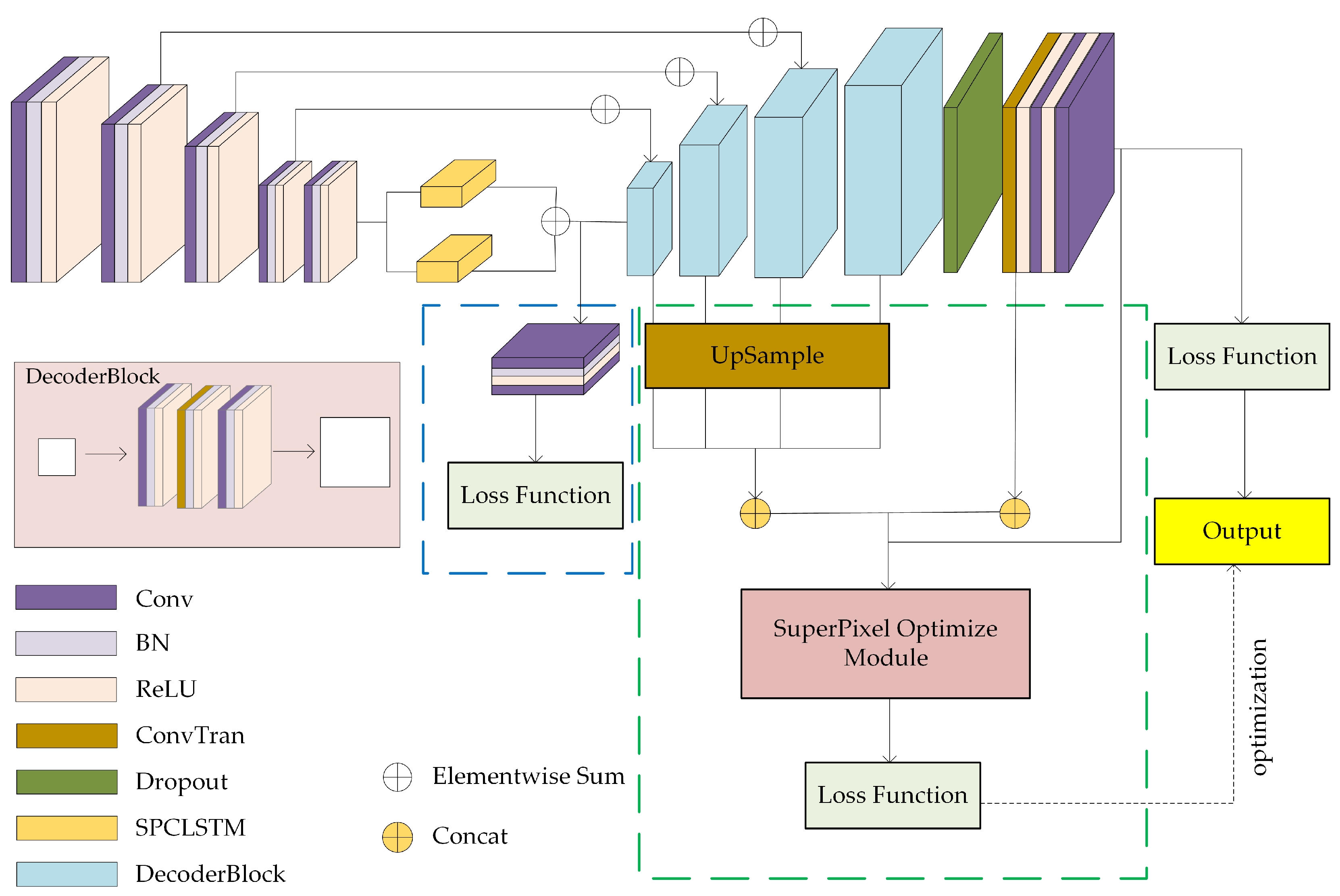
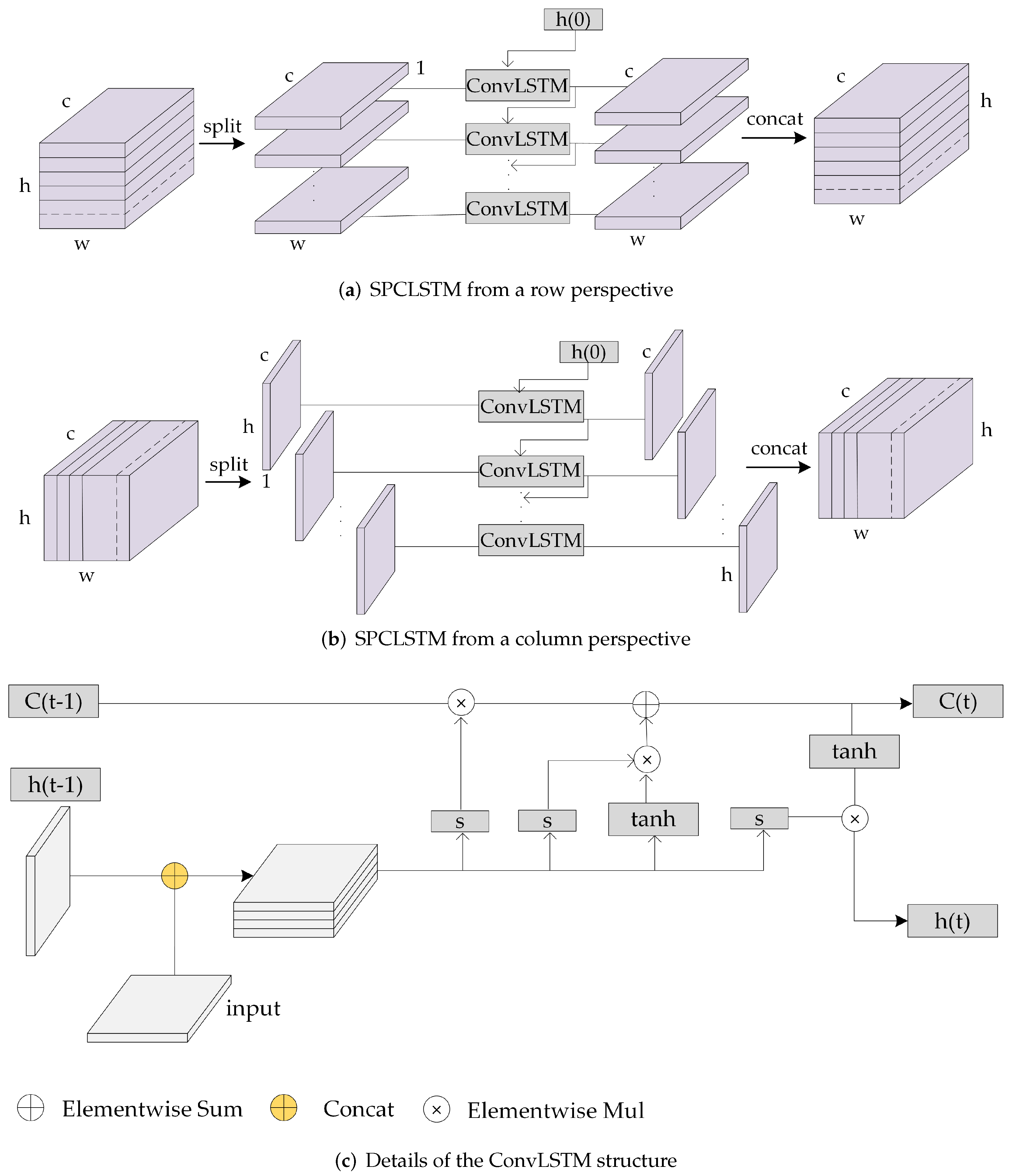
  • We propose the spatial convolutional long short-term memory (Spatial ConvLSTM, SPCLSTM) structure. The learning ability of the network for the spatial continuity of the image feature surface is enhanced by the structure of convolutional long short-term memory (ConvLSTM).
  • We introduce a multitask learning strategy in the network to compute auxiliary losses using the intermediate features extracted by the network, reducing the fuzziness of boundaries in greenhouse result extraction during training.
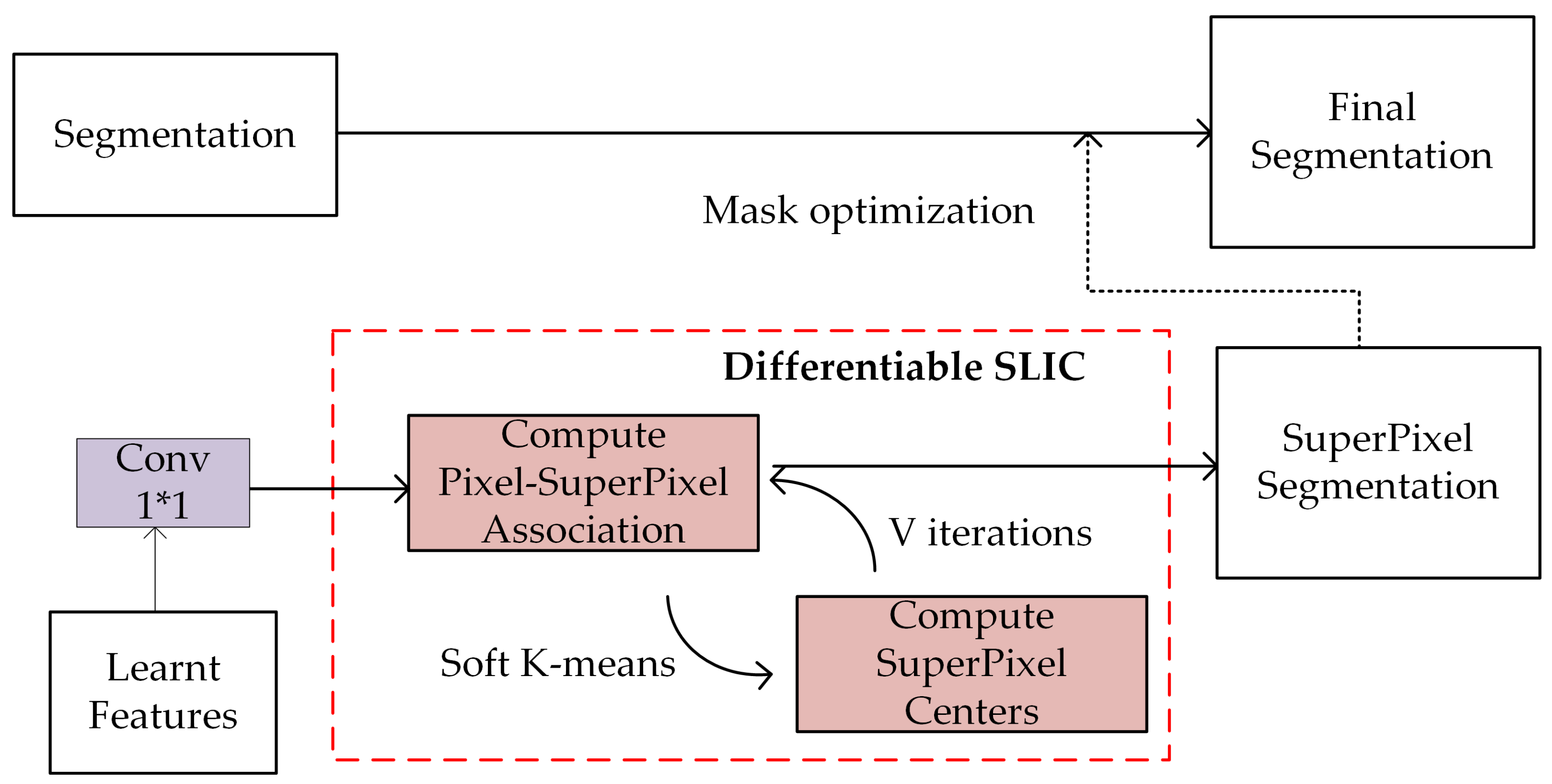
  • We propose a superpixel optimization module (SOM) that can better obtain the boundary information of the greenhouse by iterating the features of the decoder using the superpixel segmentation network. Based on this module, the greenhouse extraction results with accurate boundary information can be obtained.
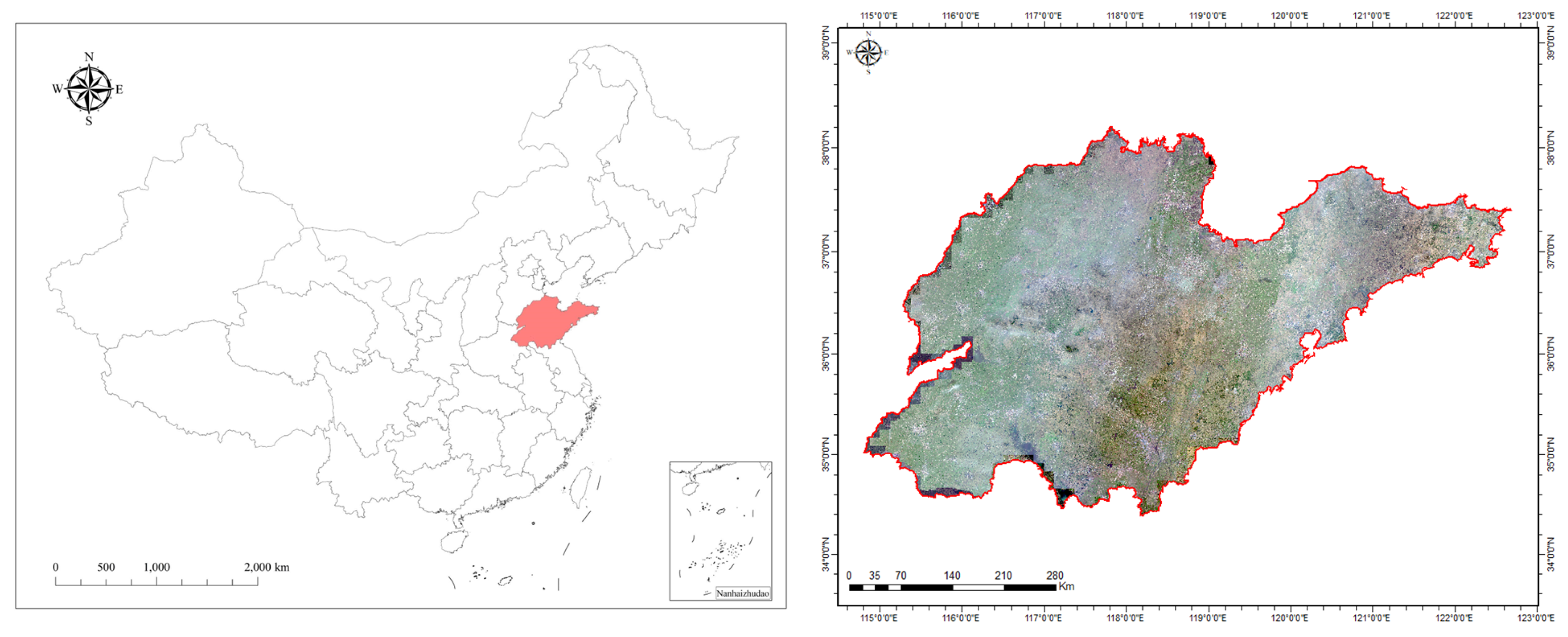
  • We also perform large-scale greenhouse mapping from 2.38 m satellite imagery in Shandong Province, China.
Put together, the proposed structure aims to make better use of the spatial information of ground objects to obtain more accurate boundary results. Compared with other mainstream methods, our network can be better applied to large-scale greenhouse extraction tasks.

2. Materials and Methods

2.1. Study Area

The study area is Shandong Province ( 34 22.9 38 24.01 , 114 47.5 122 42.3 ), China, which is located in the eastern coastal area of China, as shown in Figure 1. Shandong Province, as a major agricultural province, is an important production area for grain crops and cash crops. The area is covered with a large number of agricultural greenhouses, which have made great contributions to the agricultural development of Shandong Province. Therefore, we chose Shandong Province as the study area to test the performance of our structure in extracting agricultural greenhouses on a large scale.

2.2. Data Sets

The image data used in this paper are the 2015 Gaofen-1 satellite (GF-1) images from Shandong Province, China, covering an area of 158,000 square kilometers. The GF-1 satellite was successfully launched in April 2013. The satellite orbit and attitude control parameters are shown in the Table 1. The panchromatic resolution of the GF-1 satellite is 2 m, and the multispectral resolution is 8 m. At the same time, the revisit period of GF-1 is only 4 days and has high temporal resolution. The specific payload technical indicators are shown in the Table 2. Combining the advantages of high spatial resolution and high temporal resolution at the same time, the high-resolution data of the GF-1 satellite have played an important role in such applications as geographic mapping and agricultural resource detection [30].
We acquired multispectral images with high spatial resolution using the technique of image fusion. All images are in the RGB color space and have a resolution of 2.38 m. The labels cover approximately 6% of the study area, with 0 representing the background and 1 representing a greenhouse. All labels are manually annotated by team members, ensuring the high quality of the dataset. We divided the samples into a training set, validation set, and test set at a ratio of 8:1:1. To feed the data into the designed neural network, we cropped the large-scale samples to image patches of size 768 × 768 pixels. Based on the above work, we randomly constructed a large-scale agricultural greenhouse dataset (LSAG dataset) containing 11,913 training samples, 1367 validation samples, and 1367 test samples.

2.3. Methods

2.3.1. Network Architecture

The structure of our proposed network is shown in Figure 2. Our network adopts an encoder–decoder structure, and ResNet34 [31] is used in our network. First, we use ResNet34 as the encoder to extract features. To better extract the spatial structure information in the images, we use the SPCLSTM module to model the spatial relationships of the feature maps from the row and column perspectives. We also use the output of the SPCLSTM module as the feature maps of the auxiliary tasks to calculate the supervised loss, accelerating the convergence of the network. Finally, we perform superpixel segmentation on the decoder results and use the exact oversegmentation results of the image to further optimize the segmentation results of the decoder.

2.3.2. Spatial ConvLSTM

Pan et al. [32] used layer-by-layer convolution instead of traditional convolution in the feature map, thus enabling information transfer between pixels across rows and columns. Zhou et al. [33] performed convolution operations on the rows and columns based on an SCNN and superimposed the output of the previous row or column onto the next row or column as the input. The results proved that this structure can solve the problem of road extraction interruption by enhancing the road geometry. Inspired by their work but in contrast to their study, we extract the spatial relationships of the feature maps from the row and column perspectives in parallel, rather than serially from first the row perspective and then the column perspective. More importantly, our module adopts the structure of ConvLSTM to consider the temporal relationship between different rows or different columns to reflect the spatial position relationship of the objects in the image.
Our SPCLSTM module is shown in Figure 3. Figure 3a,b show the two forms of the SPCLSTM module from the row and column perspectives, respectively. Figure 3c represents the structure of ConvLSTM.
Taking Figure 3a as an example, the SPCLSTM module receives the feature map of size C × H × W extracted by the encoder and outputs a tensor of size C × H × W after modeling the spatial relationships in the feature map. C, H, and W denote the number of channels and the height and width of the feature map, respectively. After partitioning the feature map from the row perspective, we can obtain sequence data representing the sequential relationships between rows. Then, the ConvLSTM structure is used to describe the order relationship between rows. The structure of ConvLSTM is shown in Figure 3c. The structure is very similar to that of LSTM, and the difference between the two lies in the intermediate computing operations. The input and output of ConvLSTM are three-dimensional tensors, and the convolution operation is used to better obtain the relationship between the spatial feature transformations of different rows or columns.
ConvLSTM was first proposed in [23], and the computational procedure of it can be formulated as follows:
i t = σ ( W x i X t + W h i H t 1 + W c i C t 1 + b i ) f t = σ ( W x f X t + W h f H t 1 + W c f C t 1 + b f ) C t = f t C t 1 + i t t a n h ( W x c X t + W h c H t 1 + b c ) o t = σ ( W x o X t + W h o H t 1 + W c o C t + b o ) H t = o t t a n h ( C t )
where * in the formula denotes the convolution operation, and ∘ denotes the Hadamard product. X t is the input tensor, H t is the hidden sate tensor, and C t is the memory cell tensor. W x and W h represent the convolution kernels corresponding to the input and hidden state, while b means the bias term. σ represents the sigmoid function. The effect of predicting the future state of a cell in the grid using local inputs and past states is achieved by the convolution operator.

2.3.3. Multitask Learning

The purpose of multitask learning is to reuse existing prior knowledge to design multiple correlated tasks for a neural network and then accelerate the training and convergence process of the network by optimizing multiple tasks simultaneously. We found that the semantic segmentation of remote sensing images is greatly affected by mixed pixels, and the object boundary is prone to blurring, which is more obvious in low-resolution images. For the greenhouse extraction task, fuzzy boundaries have an important impact on the optimization process during network training. Therefore, we add a multitask learning strategy to the network structure to reduce the effect of ambiguous image boundaries.
In Figure 2, we add a multitask learning strategy after the SPCLSTM module, which is the blue dashed box in the figure. The feature maps obtained after the spatial relationship modeling by the SPCLSTM module are merged, and then the loss function is calculated after the convolution operation. Therefore, in the whole network, the main loss is first calculated from the main branch network, which is the loss value obtained by comparing the result of the network after the decoder calculation with the real value. Second, the network contains an auxiliary loss, and the auxiliary loss value is calculated using the results after modeling the spatial relationship of the encoder’s output. Finally, we calculate the gradient propagation by summing the two loss values. Unlike the loss value of the main branch network, the calculation of the auxiliary loss value is performed after downsampling by a factor of 32. By optimizing both loss functions simultaneously through multitask learning, the model is better able to focus on the blurred boundaries of the images to obtain extraction results with precise boundaries. More importantly, multitask learning can better promote the directional propagation of gradients, which facilitates the training of the network and accelerates convergence.

2.3.4. Superpixel Optimization

Superpixel segmentation is an oversegmentation technique that obtains accurate boundary representations of image objects by clustering the image pixels. SLIC is a classical superpixel segmentation method that converts images from the RGB color space to the CIELAB color space for clustering and is also an unsupervised learning method. The SLIC method is nondifferentiable, which means that SLIC cannot be directly applied to neural networks. Inspired by the SSN [29], we add a superpixel branch to the network and use the results of superpixel segmentation to optimize the results of semantic segmentation to obtain more accurate boundary information.
In contrast to their work, our superpixel branch consists of three steps. First, all the features of the decoder are fused as the input of the differentiable SLIC module. Then, we propose a superpixel optimization module (SOM), which performs a differentiable SLIC step and an optimization step. We take the intermediate features and segmentation results as the input, and the output is the greenhouse extraction result optimized by the superpixel results. Finally, we use the optimized semantic segmentation results and the true label values to calculate the loss function values to optimize the network. The structure of the SOM is shown in Figure 4.
The inputs are all the outputs of the decoder in the network layer and the results of the semantic segmentation of the main branch network. First, the superpixel segmentation results are obtained by differentiable SLIC processing. The semantic segmentation results are then mask-optimized to obtain more accurate boundary results by using the oversegmentation results of superpixel segmentation. Our mask optimization steps can be described by Algorithm 1. Our input includes the result of the superpixel segmentation and the extracted map of the semantic segmentation network. For each mask in the semantic segmentation result, there must be a superpixel block intersecting it in the superpixel segmentation result. Therefore, first, we traverse each superpixel block R s u p ( i ) in the superpixel result and determine whether the superpixel block intersects a certain mask R s e g ( j ) in the semantic segmentation result. If there is an intersection, we calculate the Jaccard index of the intersection area and the superpixel block directly. The higher the index is, the more similar the two results are. Here, we introduce a threshold θ ; if the value of the Jaccard index is greater than the threshold, we use the boundary of the superpixel block as the final result. Otherwise, we use the boundary of the original mask in the semantic segmentation result as the final result.    
Algorithm 1: Superpixel optimization module.
Remotesensing 14 04908 i001

2.3.5. Loss Function

The loss function of our network consists of multiple parts. Greenhouse extraction is a binary semantic segmentation task in which the network aims to distinguish between the greenhouse and the background of the image. Like in [34], we use a joint loss function which is a combination of the binary cross entropy (BCE) and dice coefficient loss. The theory of BCE loss was first proposed in [35]. It has been widely used as a loss function for binary classification, such as building segmentation [36], binary change detection [37]. We first use BCE loss as the basic loss function to calculate the pixel difference between the predicted result and the true label. The BCE loss is defined as follows:
L B C E = 1 N i = 1 N ( y i l o g y i ^ + ( 1 y i ) ( 1 l o g y i ^ ) ) .
where N in the formula denotes the number of samples, y i represents the real label value, y i { 0 , 1 } , and y i ^ represents the probability value of the predicted greenhouses.
Since the BCE loss needs to determine whether each pixel value is a greenhouse and then average all the values, the final loss function value is influenced by the category with more area when the distribution of categories in the image is unbalanced. In the greenhouse extraction task, an image often contains more background information, and the greenhouse is only a minority of the image. Therefore, we add the dice loss function. Dice loss was first used in [38]. Compared with the BCE loss function, which considers the difference between individual pixels, dice considers the intersection of all pixels in the same class as the ground truth and is not affected by a large number of background pixels. The dice loss function is calculated as follows:
L d i c e = 1 2 | Y P | | Y | + | P | ,
where Y denotes the true label value, P denotes the model predicted value, and | · | represents the number of elements in the set.
Since the network adopts a multitask learning strategy, the calculation of the loss value includes the loss of multiple branches. For the main branch, we compute the difference between the predicted result and the true label. For the auxiliary branch, since the middle feature map is downsampled by a factor of 32 in the original size, we also downsample the true label value by a factor of 32 and calculate the loss value with the auxiliary feature map. For the superpixel optimization structure, we calculate the loss value between the optimized result and the label value.
Therefore, the loss function of the network can be expressed as follows:
L j o i n t = L B C E 1 + L d i c e 1 + λ 1 × ( L B C E 2 + L d i c e 2 ) + λ 2 × ( L B C E 3 + L d i c e 3 ) ,
where L B C E 1 , L d i c e 1 , L B C E 2 , and L d i c e 2 represent the BCE and dice losses of the main branch and the BCE and dice loss values of the auxiliary branch, respectively. L B C E 3 and L d i c e 3 denote the BCE and dice loss values, respectively, between the superpixel optimization results and the label values. λ 1 and λ 2 represent the proportions of the loss values of the multitask learning structure and the superpixel optimization structure, respectively.

2.3.6. Evaluation Metrics

In our experiments, the F1 score and intersection over union (IoU) are used as the evaluation metrics. The F1 score is the harmonic mean of precision and recall, with a minimum value of 0 and a maximum value of 1. IoU represents the ratio of the intersection of the predicted results and the true value to the union. Both of them are the most common evaluation metrics in semantic segmentation [39], and the relevant formulas are as follows:
P r e c i s i o n = T P T P + F P
R e c a l l = T P T P + F N
F 1 = 2 P r e c i s i o n R e c a l l P r e c i s i o n + R e c a l l
I o U = T P T P + F P + F N
In the formula, TP, FP, and FN represent the numbers of true positives, false positives, and false negatives, respectively. TP represents the number of correctly identified greenhouse pixels, FP represents the number of non-greenhouse pixels incorrectly identified as greenhouses, and FN denotes the number of greenhouse pixels incorrectly identified as non-greenhouse pixels. Precision measures the percentage of correctly classified pixels in the prediction results, and recall indicates the percentage of correctly predicted pixels among the pixels that are the greenhouse results.

2.3.7. Train Details

All neural networks used in the experiments in this paper were built using the PyTorch deep learning framework [40]. In the training phase, we used all training samples and validation samples.
Before the samples were fed into the network, we performed data augmentation to increase the number of samples. The data augmentation methods we employed included random flipping, rotation, scaling, and random cropping of the samples to a size of 512 × 512. During testing, we used all 768 × 768 samples to obtain the output and used only the output of the main branch to calculate the test accuracy. During the inference on the province-wide range, we used the overlap-tile strategy to crop the large images to a size of 1024 × 1024, which could effectively solve the problem of poor edge performance in the extraction results of the greenhouses.
We trained our network on 2 NVIDIA TITAN XP GPUs (12 GB memory). For the proposed network architecture, the size of a mini-batch can be as large as 12. We chose BCE and dice as the loss functions and used AdamW [41] as the optimizer, with the initial learning rate set to 0.001 and the weight decay to 0. The learning rate was adjusted by observing whether the F1 score of the validation set increased within 20 epochs. If there was no increase, then the learning rate was adjusted to half of the previous rate. In addition, we used a warm-up strategy in the first 500 training iterations, which can reduce the probability of the network falling into a local optimum and can help the network train better. Meanwhile, batch normalization [42] was used to help the network accelerate convergence. For the hyperparameter settings in the superpixel optimization module, we set the value of the threshold θ to 0.5. For the hyperparameter setting of the loss function, we set the values of λ 1 and λ 2 to 0.2.

3. Results

3.1. Ablation Study

3.1.1. Quantitative Comparisons

To test the generalization ability of the proposed module on greenhouse extraction, we tested the performance of different modules on our own large-scale agricultural greenhouse dataset (LSAG dataset). We adopted the UNet structure as the baseline network and used ResNet34 as the encoder. On this basis, the modules we proposed were added, and the results for the Shandong Gaofen-1 satellite dataset are shown in Table 3.
The baseline network UNet can achieve an F1 score of 74.92% on our dataset, while the experimental accuracy can reach 77.40% after adding the SPCLSTM module. In the ablation experiments, we set the number of layers of the SPCLSTM module to 2. The SPCLSTM module can model the spatial information of the greenhouse in the image from the perspective of rows and columns and better extract the image features of the greenhouse to ensure that the greenhouse results have the correct spatial information. From the quantitative results, the SPCLSTM module can effectively improve the precision and recall of the greenhouse extraction results. That is, the SPCLSTM can effectively reduce false detection and missed detection in greenhouse extraction. When adding a multitask learning strategy to our architecture, we can achieve an accuracy of 76.03% in terms of F1 score on our LSAG dataset. Compared with the baseline structure UNet and the results after adding the SPCLSTM module, the network using the multitask strategy has a higher precision in the prediction results, while the recall rate is significantly lower. The multitask structure is more sensitive to the boundary information in the image and has stricter requirements for the shape of the greenhouse due to the addition of the intermediate result calculation loss in the process of network feature extraction, resulting in more missing information in the process of extracting the model. In the fourth row in Table 3, we combine the SPCLSTM and the multitask learning strategy. Compared with adding the SPCLSTM module or the multitask learning strategy separately, the combination of the two modules can better balance the precision and recall of greenhouse extraction to improve the final accuracy of the network. Finally, we added a superpixel segmentation structure to obtain the best results. We first performed superpixel segmentation on the feature map of the decoder to obtain the oversegmentation results and then used the oversegmentation results to optimize the results of the main network semantic segmentation. Benefiting from the more precise boundary information in the oversegmentation results of superpixel segmentation, the results in the table show that our superpixel segmentation optimization strategy improves both precision and recall. The F1 score improved by approximately 4% over the baseline.

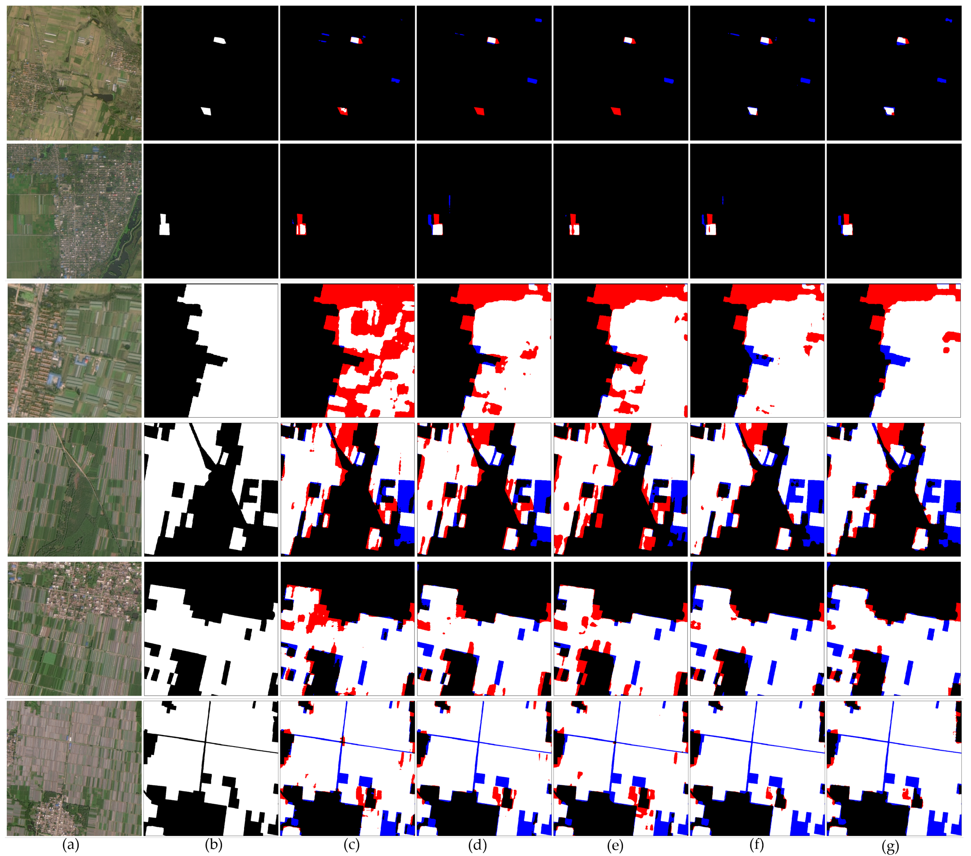
3.1.2. Visualization Results

To qualitatively compare the effects of different modules, some result graphs of the ablation experiments are shown in Figure 5. On the whole, the network with the SPCLSTM module, multitask learning strategy, and superpixel segmentation structure added in the last column can achieve the most accurate greenhouse extraction effect, but there are still cases of false detections and missed detections.
In the validation set results shown in Figure 5, we divide the example images into three groups. The first and second rows represent scenes with a sparse distribution of greenhouses. The third, fourth, and fifth rows are a group, representing a scene in which the greenhouse and other objects coexist with a small difference in the distribution range. The last row represents the large-scale greenhouse extraction task.
In the first and second rows, the greenhouses are sparsely distributed in the image. The baseline UNet has many missed detections and cannot completely extract the small and sporadically distributed greenhouse shapes. In the first row, the SPCLSTM structure can reduce false detections in the area near the greenhouse because it can model the spatial characteristics of the greenhouse. The multitask learning strategy has stricter constraints on the boundary information of the greenhouse and has a higher degree of discrimination for small objects with similar textures in the image. Therefore, similar greenhouses and buildings can be better distinguished. However, the current single structure generally has some missed detections. After combining the SPCLSTM and a multitask learning strategy, the network has a better learning ability for the spatial shape information and boundary information of the greenhouse. For sparsely distributed greenhouses, more complete results can be extracted. Finally, the SOM is added to optimize the semantic segmentation results by using the obtained oversegmentation results. The network can effectively reduce the false detection of buildings with similar textures. In the second row, there are a large number of residential areas in the original image, and there are cultivated areas with similar structural information near the greenhouse. The SPCLSTM structure has a better ability to extract the spatial information of the greenhouse and can help obtain the results of greenhouses with regular geometric shapes. The multitask learning strategy adds an additional loss function to optimize the network, and the extracted greenhouse results can fit the label values well on the edges. After combining the two and using the SOM, our network is able to achieve a better balance between precision and recall. The extracted greenhouse results are smoother and have a regular geometry.
In the second set of examples, the greenhouse occupies a large area in the image, and there are also large-scale residential areas or cultivated or grassland areas in the image. From the overall results, the baseline UNet has a large number of missed detections in the application of large-scale greenhouse extraction. The main reason is that the texture information of the greenhouses in the images is quite different, and simply extracting the greenhouses based on the texture information can lead to missed detections. The structure we propose can gradually reduce the missed detections, and the extracted results are gradually regularized to better fit the edge of the greenhouse. In the third row, there are a large number of irregularly distributed greenhouses in the image. The extraction results of the baseline are very scattered and not smooth, and there are many missed detections on the edges. The SPCLSTM structure can better consider the shape information of the greenhouse in the image. Therefore, the SPCLSTM module has a good extraction ability, whether the greenhouse in the image is vertical or horizontal. Although the multitask learning strategy still has a large number of missed detections, the extracted greenhouse results are more accurate on the edges. After combining the SPCLSTM module and the multitask learning strategy, the extracted greenhouse results can better fit the real edge information. Finally, our proposed SOM can effectively eliminate the missed detection of small areas in the extraction of greenhouses. In the fourth row, the greenhouses in the image are distributed in a large area of vertical strips, and the baseline is likely to miss some greenhouses with dissimilar texture information. Since the SPCLSTM module can better extract regularly shaped greenhouses and the multitask learning strategy can ensure that the extracted greenhouse results have better edge information, the results are significantly improved after combining the SPCLSTM module and the multitask learning strategy. With the addition of the SOM, the network also has a stronger ability to identify areas with large differences in texture information in the distribution area of the greenhouse, which can reduce the missed detections in the distribution area. In the fifth row, there are a large number of residential areas in the vicinity of the greenhouse. Moreover, the color information of the residential area has a high similarity to that of the greenhouse, which makes the extraction of the greenhouse in this area difficult. From the results, it can be found that the baseline has more missed inspections in the adjacent parts of the residential area and the greenhouse. The SPCLSTM module can consider the spatial information of residential areas and greenhouses and has a higher ability to distinguish between residential areas and greenhouses. After incorporating a multitask learning strategy, the extracted greenhouse results have higher accuracy on the edges. The superpixel segmentation optimization strategy can further optimize the edge information of the extracted results. At the same time, it can eliminate missed detections in the greenhouse area. However, these groups of extraction results have false detections for non-greenhouses in the greenhouse area, and these false detections in the greenhouse area need further study.
In the last set of images, we show the effect of different structures on large-scale greenhouse extraction. In the last row, the greenhouse occupies most of the area in the image, and there is also a small part of a residential area and grass. The baseline has more missed detections in the large-scale greenhouse extraction results. The main reason is that UNet only considers the texture information of the objects in the image, and there may be objects with different texture information in the distribution area of the greenhouse. After considering the spatial information of the greenhouse, the SPCLSTM can significantly reduce the missed detections in the greenhouse extraction, and the geometry of the extracted large-scale greenhouse results is more regular. After considering the edge information of the greenhouse, the multitask learning strategy can effectively improve the results of extracting the edge compared with the baseline. Finally, the SOM can be used to further optimize the edge information of the extraction results. Our proposed network structure can gradually eliminate the missed detection of large greenhouse areas in the image to improve the greenhouse extraction results.

3.2. Comparing Methods

3.2.1. Quantitative Comparisons

We perform qualitative and quantitative comparisons with other state-of-the-art methods on the LSAG dataset. The mainstream methods compared include UNet [14], PAN [18], DeepLabV3+ [43], UNet++ [44], HRNet [45], and AFNet [46]. UNet adopts an encoder–decoder structure and fuses the corresponding features of the encoder during the upsampling process of the decoder, which can preserve the low-level features and high-level semantic features of the image. PAN adopts a feature pyramid attention (FPA) module in the network to consider the contextual information at different scales and adopts a global attention upsampling (GAU) module in the decoder structure to fully fuse low-level and high-level feature information. DeepLabV3+ adopts an encoder–decoder structure and controls the size of the receptive field through atrous convolution. UNet++ improves upon UNet by adding dense convolutional layer connections and is able to balance the accuracy and speed of the network through pruning operations. HRNet connects multi-resolution convolutional streams in parallel, so the feature representation has richer semantic information and more accurate spatial structure. AFNet fuses features at different levels to improve the classification accuracy of target objects at the boundary. Our comparison results are shown in Table 4.
In the table, train time represents the time for our model to train an epoch, and test time represents the running time of the model on the test set. In terms of accuracy, our network achieves the best results compared to state-of-the-art methods. The training time and testing time of the proposed structure are slightly worse than those of UNet and PAN. The network structures of HRNet and AFNet are relatively complex, and the amount of parameters and training time are very large. This is very inconvenient for large-scale greenhouse extraction tasks. Considering the balance between time and accuracy, our network is more competitive than the mainstream methods.

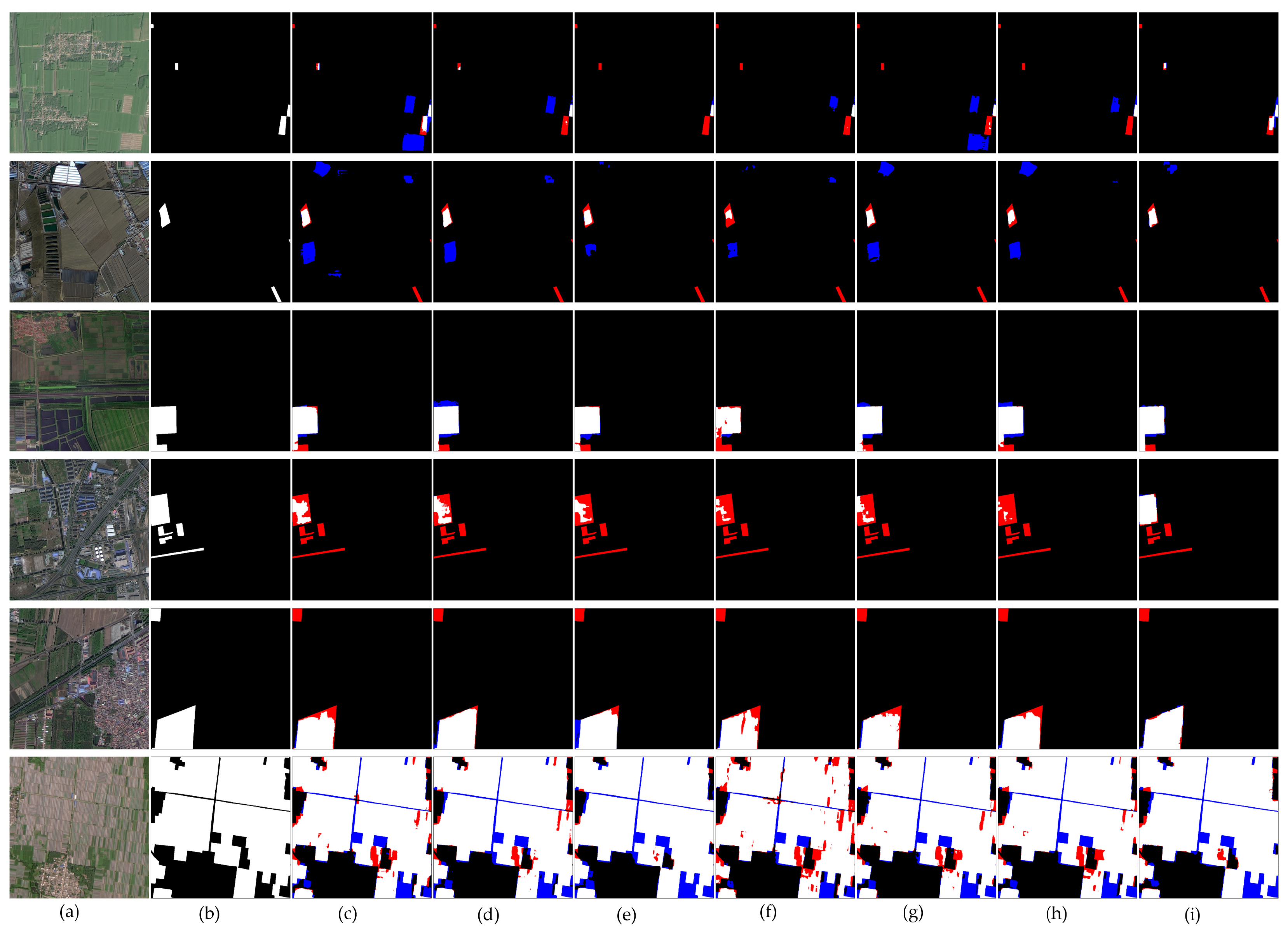
3.2.2. Visualization Results

A comparison of our visualization results is shown in Figure 6. On the whole, our method can effectively reduce the missed detections and false detections in the greenhouse extraction results of the network, whether it is performing a small-area greenhouse extraction task or a large-scale greenhouse extraction task.
In Figure 6, we divide the comparison results into three groups. The first and second rows are a group representing a sparsely distributed area of small greenhouses, and there are many similar objects in the image. The third, fourth, and fifth rows are a group representing a scene in which small-area greenhouses are densely distributed in a certain area, and the greenhouses within this distribution range are slightly different in texture. The last row represents a large-scale greenhouse extraction task. In the first and second rows, all methods have some false detections and missed detections, but our network is able to minimize the false and missed detections. In the first row, the surrounding arable land will affect the extraction of the target greenhouse, and the mainstream network generally misclassifies the cultivated land as greenhouses. In the second row, the similar buildings in the image will also affect the extraction of the target greenhouse. The mainstream networks mistakenly classify similar buildings around the greenhouse as greenhouses. Our network establishes a spatial relationship between the rows and columns to model the spatial characteristics of the greenhouse, which can effectively reduce false detections in the extraction results of the greenhouse. However, in this set of experiments, all the results have missed detections, such as in the bottom right area of the second row. In this scenario, the information of the greenhouse is not very different from that of the surrounding area, except for the color, and the existing network structure has difficulty distinguishing it directly based on color and texture.
In the second set of experiments, our network can extract more accurate greenhouse results than the mainstream networks. The mainstream networks have some missed detections in the greenhouse extraction task in this complex scene. In the third row, there are a few buildings near the greenhouse area in the image that affect the extraction results. At the same time, the greenhouses in the area have different color information, and there are large gaps between the greenhouses in the area. Due to the use of attention, PAN is more sensitive to the details in the image, and the extracted large-scale greenhouse results are prone to fragmentation. In the results of the fourth row, the information of the image is relatively complex, and the texture information of the greenhouse area is quite different, so it is easy to miss detection. In this scenario, the greenhouse extraction effect of the mainstream networks shows some missed detections, and the extraction results are very irregular. In contrast, our network has a stronger geometric modeling ability to extract greenhouse results with a more accurate geometry in complex scenes. In the fifth row, the color information of the greenhouse in the image is quite different, and the difference from the cultivated land in the surrounding area is very small. All networks can correctly extract the location of the greenhouse area, but the extraction results of the mainstream networks do not match the label values on the edge. The main reason is that the texture information of this part of the image is very different from that of most greenhouse areas, and it is difficult for mainstream networks to directly extract such areas with large differences. Our network can extract greenhouse results with more accurate boundaries and geometry based on the spatial distribution information of the features due to its ability to fully consider the spatial information of the feature targets in the images. However, in this set of experimental results, all networks have missed detections to some extent. Because the greenhouse information in this small area is quite different from the main area where the greenhouse is distributed, it is difficult for the network to judge whether the area is a greenhouse based on the texture information in the image. Although there are still a small number of missed detections, our network greatly improves compared to mainstream networks. The small number of missed detections can be improved by further research on how to effectively combine other types of data to obtain more information.
In the last row, we show the results of different network structures on the large-scale greenhouse extraction task. The mainstream networks all have missed detections in the results of large-scale greenhouse extraction tasks, resulting in extraction results that appear very broken. In particular, the mainstream networks are more likely to miss greenhouses with slightly different texture information in large areas. Our network combined with a multitask learning strategy and SOM can effectively ensure that there are no scattered missed detections in the extraction results. However, these groups of networks have poor distinctions between greenhouses and roads, and roads are wrongly classified as greenhouses. Because the color information of a greenhouse and a road in an image is similar and the shapes of both are slender, the network cannot distinguish them simply based on the texture information and spatial information. Therefore, it is necessary to further limit the spatial information of the greenhouse to distinguish the greenhouse from other objects with similar shapes.

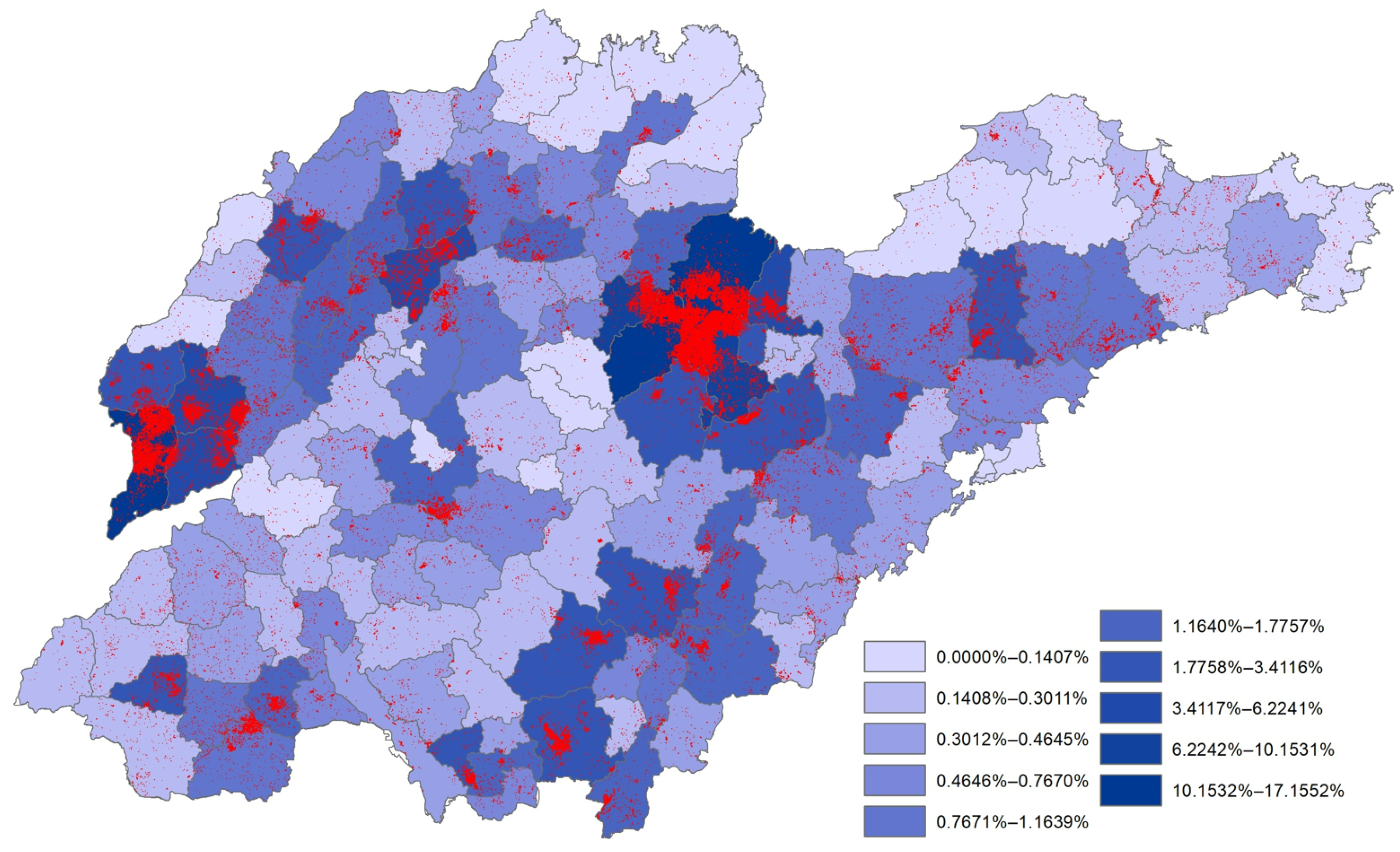
3.3. Large-Scale Greenhouse Mapping

We completed the mapping of a 2.38 m greenhouse in Shandong Province, China, using the proposed network structure, and the results are shown in Figure 7. In the figure, the red area represents the greenhouse results extracted in the study area, accounting for 1.35% of the total study area. We also show the proportion of greenhouse area in different counties at the county level. The deeper blue an area in the figure is, the higher the proportion of the greenhouse area at the county level.

4. Discussion

4.1. Numbers of SPCLSTM Layers

In our network, the complexity of the network model can be enhanced by stacking SPCLSTM modules. Although complex networks have a stronger ability to model the spatial features of images, choosing appropriate parameter values is still a problem that needs to be considered. Here, we experimentally test the effect of the number of stacked SPCLSTM modules on the network performance and model complexity. The results are shown in Table 5. To eliminate the influence of the multitask learning strategy and superpixel optimization module, we only add the SPCLSTM module based on UNet in our experiment.
As the number of SPCLSTM modules increases, the number of parameters of the network does not change, while the train time and test time have a significant tendency to increase. The train time here refers to the time it takes for the model to train an epoch. One epoch means that all data are used once. While the test time here represents the running time of our structure on the test set. In terms of accuracy, a higher level is reached when the number of SPCLSTM modules is increased to 2. After that, the performance of the network decreases slightly as the number of SPCLSTM modules continues to increase. Therefore, we set the number of SPCLSTM modules to 2 as the hyperparameter setting of our experiments to ensure that the model has a high accuracy rate and the test time is within an acceptable range.

4.2. Applications

The network structure proposed in this paper is mainly suitable for large-scale greenhouse extraction tasks and has a strong ability to distinguish complex objects in large-scale remote sensing images. The main advantage of our network over other mainstream networks is that it can obtain greenhouse extraction results with accurate and complete geometry and boundary information.
Our proposed structure is suitable for different scenarios. First, for sparsely distributed greenhouse extraction tasks, ordinary convolutional neural networks cannot effectively extract complete greenhouses. At the same time, it is easy to falsely detect ground objects with similar texture information in the image. This situation occurs mainly because sparsely distributed greenhouses generally account for a small proportion of the images. More importantly, this type of greenhouse is often not very different from the surrounding environment, which makes it difficult for ordinary convolutional neural networks to directly extract complete greenhouse results. Second, for an extraction task with a dense distribution of greenhouses in a certain area, the mainstream convolutional neural network is often affected by the difference in the texture information of the greenhouses in the region, resulting in more missed detections. From the experimental results, our method can effectively ignore the color difference of greenhouses in the same area to reduce the proportion of missed parts. Finally, for the large-scale greenhouse extraction task, the mainstream convolutional neural network is easily affected by large differences in the greenhouses in the region during the extraction process, and there are more missed detection cases. From the experimental point of view, the main problem with the existing mainstream networks in various scenes of greenhouse extraction applications is the high number of missed detections in the extraction process for greenhouses with different texture information. Our network has a good improvement effect in a variety of scene applications.
Our proposed structure is also applicable to different remote sensing image datasets. For other types of remote sensing images, such as multispectral or hyperspectral, our proposed structure still has strong applicability. In optical images, there are often some objects that are difficult to distinguish through RGB bands, such as greenhouses and plastic films. They tend to have similar texture and shape information in images. However, hyperspectral images and multispectral images often have information of different spectral bands, which is beneficial to the distinction of different ground objects. For different types of image data, the network structure we adopt can be applied by changing the number of input channels. At the same time, our proposed SPCLSTM structure can preserve the spectral information of the corresponding ground objects. For multispectral images, the SPCLSTM structure can firstly model the spatial information of ground objects by considering the relationship between image rows and columns. At the same time, the SPCLSTM structure can reserve all the spectral information of each ground object. Further, the SPCLSTM structure can obtain the continuity information of spectral bands in multispectral or hyperspectral images by dividing the features from the perspective of spectral bands.
Our proposed network is similar to the UNet structure in that it has the form of an encoder–decoder network, but the different modules used in the network can effectively improve its performance and can be easily embedded in other frameworks. The SPCLSTM module considers the spatial characteristics of the greenhouse structure from the perspective of rows and columns, which strengthens the network’s ability to learn the spatial information of the greenhouse. In the small-area greenhouse extraction task, it is less affected by the surrounding environment, ensuring that the extraction results will not be affected by the existence of similar ground objects. In large-scale greenhouse extraction applications, greenhouses with large differences can also be accurately extracted through similar spatial information. The multitask learning strategy calculates the loss value between the features with spatial information and the label value, which promotes gradient propagation and accelerates the convergence of the network. It is most important to ensure that the extraction results of the greenhouse have more accurate boundaries. For sparsely distributed greenhouse extraction applications, the multitask learning strategy has stricter constraints on boundary information to ensure fewer false detections in the network. For large-scale greenhouse extraction tasks, the multitask learning strategy can obtain more precise boundaries during the extraction process. According to the experimental results, the adoption of the SPCLSTM module and multitask learning strategy can yield very accurate greenhouse extraction results by simultaneously considering the spatial geometric information and edge information of the greenhouse. Finally, the superpixel optimization strategy further ensures the accuracy of the semantic segmentation results on the boundary. We combine all the decoder outputs as the input of the superpixel optimization module and then perform superpixel segmentation through differentiable SLIC. The semantic segmentation results are then optimized using our proposed optimization strategy. In the optimization process, the superpixel segmentation results and the semantic segmentation results are essentially complementary. The superpixel segmentation results add more precise boundary information to the semantic segmentation results, and the semantic segmentation results assign the extracted semantic information to the superpixel segmentation results. In the network, a convolutional layer is added to the superpixel optimization branch to indicate that the branch is learnable. For sparsely distributed greenhouse extraction tasks, the SOM can effectively reduce the false detection of small targets. Additionally, for large-scale greenhouse extraction applications, the SOM can further fill in the missed targets in the area.
In general, the proposed network module, including the SPCLSTM, multitask learning structure, and SOM, can gradually optimize the spatial geometric information and edge information of the greenhouse to obtain the best extraction results for both sparsely distributed greenhouse regions and large densely distributed greenhouse regions. The experiments prove that our structure has strong robustness in practical applications.

4.3. Limitations

Although our study has strong advantages in large-scale greenhouse extraction, the proposed structure still has some drawbacks. Similar to the extraction results of all mainstream networks, our network structure still has a small number of false detections on the large-area greenhouse extraction task. For greenhouses and adjacent cultivated land in concentrated areas, there are still some cases of misclassification of cultivated land as greenhouses in our network structure. For greenhouse extraction tasks in large areas, the network structure cannot distinguish roads and greenhouses well. Because the greenhouses and roads in the images are both slender objects and are similar in texture, simply applying a combination of spatial and texture information cannot distinguish the two well.
In future research, we will first focus on the extraction of the spatial information of ground objects. For slender targets, we will determine how to properly extract spatial information to improve the discrimination between similar targets through information such as the length and width of the targets. A second task is the fusion of spatial information and texture information. There are many methods of data fusion, and our network only aims to model spatial features after the texture information is extracted. In future research, various methods of information fusion will be tested. Finally, we aim to improve the superpixel optimization strategy. The currently adopted optimization strategy is still established artificially, and this strategy is often influenced by the subjective features of researchers. In future research, we will study how to use non-artificial strategies for optimization.

5. Conclusions

Large-scale greenhouse extraction is crucial for the sustainable development of modern agriculture. However, existing greenhouse extraction networks do not fully consider the spatial relationship of the objects in remote sensing images, and the extracted greenhouse results have errors on the boundaries, with relatively limited accuracy. In this paper, we first construct a large-scale agricultural greenhouse dataset named LSAG. To better model the spatial relationship of remote sensing ground objects, we propose the SPCLSTM structure. It can calculate the correlation between different rows or different columns of an image and has a stronger ability to extract the spatial features of objects. The extracted greenhouse results have more accurate boundary information. In addition, we adopt a multitask learning strategy in the network training process to calculate the loss value between network features with spatial information and label values. The auxiliary loss is used to optimize the training of the network and accelerate convergence. At the end of the network, we add a superpixel optimization branch to obtain more accurate boundary results for greenhouse extraction. We propose a learnable superpixel optimization module to perform superpixel segmentation on the stacked decoder features and use the superpixel segmentation results to optimize the semantic segmentation results of the main branch network to obtain greenhouse extraction results with precise boundaries.
The experimental results show that our proposed structure achieves state-of-the-art performance, with an F1 score as high as 78.66% on our large-scale agricultural greenhouse dataset, which proves that the proposed module can effectively help the semantic segmentation network to obtain greenhouse extraction results with precise boundaries. The SPCLSTM module models the spatial features of ground objects, while the multitask learning strategy and the superpixel optimization module can obtain results with more accurate boundary information. The results of province-wide large-scale greenhouse extraction also demonstrate the feasibility of our structures in application. In future research, a deeper study on the application of superpixel optimization to greenhouse extraction will be considered to obtain a more efficient model, and the application of our network structure for greenhouse extraction at the national level will be considered.

Author Contributions

Conceptualization, M.C. and J.G.; methodology, M.C. and J.G.; validation, X.Y. and P.C.; formal analysis, Q.L.; resources, Z.C.; data curation, P.C.; writing—original draft preparation, M.C. and Z.W.; writing—review and editing, Z.W.; visualization, Z.W.; supervision, X.Y.; project administration, Z.C.; funding acquisition, Z.C. All authors have read and agreed to the published version of the manuscript.

Funding

This research was funded by the the National Key Research and Development Program of China (Grant No. 2021YFB390110302).

Data Availability Statement

Not applicable.

Acknowledgments

The authors are grateful to the editors and anonymous reviewers for their informative suggestions.

Conflicts of Interest

The authors declare no conflict of interest.

Abbreviations

The following abbreviations are used in this manuscript:
BCEbinary cross entropy
CNNconvolutional neural network
ConvLSTconvolutional long short-term memory
FCNfully convolutional neural network
FNfalse negative
FPfalse positive
FPAfeature pyramid attention
GAUglobal attention upsampling
IoUintersection over union
LSAGlarge-scale agricultural greenhouse
LSTMlong short-term memory
PANpyramid attention network
PSPNetpyramid scene parsing network
ReLURectified Linear Unit
RNNrecurrent neural network
SARsynthetic aperture radar
SCNNspatial convolutional neural network
SLICsimple linear iterative clustering
SOMsuperpixel optimization module
SPCLSTMspatial convolutional long short-term memory
SSNsuperpixel sampling network
TPtrue positive
UAVunmanned aerial systems

References

  1. National Bureau of Statistics. Communiqué on Major Data of the Third National Agricultural Census (No. 2). Available online: http://www.stats.gov.cn/tjsj/tjgb/nypcgb/qgnypcgb/201712/t20171215_1563539.html (accessed on 29 June 2022).
  2. Sun, X.; Lai, P.; Wang, S.; Song, L.; Ma, M.; Han, X. Monitoring of Extreme Agricultural Drought of the Past 20 Years in Southwest China Using GLDAS Soil Moisture. Remote Sens. 2022, 14, 1323. [Google Scholar] [CrossRef]
  3. Hansen, M.C.; Potapov, P.V.; Pickens, A.H.; Tyukavina, A.; Hernandez-Serna, A.; Zalles, V.; Turubanova, S.; Kommareddy, I.; Stehman, S.V.; Song, X.P.; et al. Global land use extent and dispersion within natural land cover using Landsat data. Environ. Res. Lett. 2022, 17, 034050. [Google Scholar] [CrossRef]
  4. Xiang, M.; Deng, Q.; Duan, L.; Yang, J.; Wang, C.; Liu, J.; Liu, M. Dynamic monitoring and analysis of the earthquake Worst-hit area based on remote sensing. Alex. Eng. J. 2022, 61, 8691–8702. [Google Scholar] [CrossRef]
  5. Liu, G.; Li, J.; Nie, P. Tracking the history of urban expansion in Guangzhou (China) during 1665–2017: Evidence from historical maps and remote sensing images. Land Use Policy 2022, 112, 105773. [Google Scholar] [CrossRef]
  6. Zhao, G.-X.; Li, J.; Li, T.; Yue, Y.-D.; Warner, T. Utilizing landsat TM imagery to map greenhouses in Qingzhou, Shandong Province, China. Pedosphere 2004, 14, 363–369. [Google Scholar]
  7. Sekar, C.S.; Kankara, R.S.; Kalaivanan, P. Pixel-based classification techniques for automated shoreline extraction on open sandy coast using different optical satellite images. Arab. J. Geosci. 2022, 15, 1–19. [Google Scholar] [CrossRef]
  8. Lv, Z.; Yang, X.; Zhang, X.; Benediktsson, J.A. Object-Based Sorted-Histogram Similarity Measurement for Detecting Land Cover Change with VHR Remote Sensing Images. IEEE Geosci. Remote Sens. Lett. 2022, 19, 1–5. [Google Scholar] [CrossRef]
  9. Aguilar, M.A.; Jiménez-Lao, R.; Ladisa, C.; Aguilar, F.J.; Tarantino, E. Comparison of spectral indices extracted from Sentinel-2 images to map plastic covered greenhouses through an object-based approach. Gisci. Remote Sens. 2022, 59, 822–842. [Google Scholar] [CrossRef]
  10. Chen, Z.; Li, F. Mapping Plastic-Mulched Farmland with C-Band Full Polarization SAR Remote Sensing Data. Remote Sens. 2017, 9, 1264. [Google Scholar]
  11. Coslu, M.; Sonmez, N.; Koc-San, D. Object-based greenhouse classification from high resolution satellite imagery: A case study Antalya-Turkey. Int. Arch. Photogramm. Remote Sens. Spatial Inf. Sci. 2016, XLI-B7, 183–187. [Google Scholar]
  12. Aguilar, M.A.; Nemmaoui, A.; Novelli, A.; Aguilar, F.J.; García Lorca, A. Object-based greenhouse mapping using very high resolution satellite data and Landsat 8 time series. Remote Sens. 2016, 8, 513. [Google Scholar] [CrossRef]
  13. Long, J.; Shelhamer, E.; Darrell, T. Fully convolutional networks for semantic segmentation. In Proceedings of the IEEE Conference on Computer Vision And Pattern Recognition, Boston, MA, USA, 7–12 June 2015; pp. 3431–3440. [Google Scholar]
  14. Ronneberger, O.; Fischer, P.; Brox, T. U-net: Convolutional networks for biomedical image segmentation. In Proceedings of the International Conference on Medical image computing and Computer-Assisted Intervention, Munich, Germany, 5–9 October 2015; pp. 234–241. [Google Scholar]
  15. Chaurasia, A.; Culurciello, E. Linknet: Exploiting encoder representations for efficient semantic segmentation. In Proceedings of the IEEE Visual Communications and Image Processing (VCIP), St. Petersburg, FL, USA, 10–13 December 2017; pp. 1–4. [Google Scholar]
  16. Zhao, H.; Shi, J.; Qi, X.; Wang, X.; Jia, J. Pyramid scene parsing network. In Proceedings of the IEEE Conference on Computer Vision and Pattern Recognition, Honolulu, HI, USA, 21–26 July 2017; pp. 2881–2890. [Google Scholar]
  17. Chen, L.C.; Papandreou, G.; Schroff, F.; Adam, H. Rethinking atrous convolution for semantic image segmentation. arXiv 2017, arXiv:1706.05587. [Google Scholar]
  18. Li, H.; Xiong, P.; An, J.; Wang, L. Pyramid attention network for semantic segmentation. arXiv 2018, arXiv:1805.10180. [Google Scholar]
  19. Sun, Y.; Han, J.; Chen, Z. Monitoring method for UAV image of greenhouse and plastic-mulched Landcover based on deep learning. Trans. Chin. Soc. Agric. Mach. 2018, 49, 133–140. [Google Scholar]
  20. Baghirli, O.; Ibrahimli, I.; Mammadzada, T. Greenhouse Segmentation on High-Resolution Optical Satellite Imagery Using Deep Learning Techniques. arXiv 2020, arXiv:2007.11222. [Google Scholar]
  21. Zhang, X.; Cheng, B.; Chen, J.; Liang, C. High-Resolution Boundary Refined Convolutional Neural Network for Automatic Agricultural Greenhouses Extraction from GaoFen-2 Satellite Imageries. Remote Sens. 2021, 13, 4237. [Google Scholar] [CrossRef]
  22. Sun, K.; Zhao, Y.; Jiang, B.; Cheng, T.; Xiao, B.; Liu, D.; Mu, Y.; Wang, X.; Liu, W.; Wang, J. High-resolution representations for labeling pixels and regions. arXiv 2019, arXiv:1904.04514. [Google Scholar]
  23. Shi, X.; Chen, Z.; Wang, H.; Yeung, D.Y.; Wong, W.K.; Woo, W.C. Convolutional LSTM network: A machine learning approach for precipitation nowcasting. In Proceedings of the 28th International Conference on Neural Information Processing Systems, Sanur, Indonesia, 8–12 December 2021; pp. 802–810. [Google Scholar]
  24. Azad, R.; Asadi-Aghbolaghi, M.; Fathy, M.; Escalera, S. Bi-directional convlstm u-net with densley connected convolutions. In Proceedings of the IEEE/CVF International Conference on Computer Vision Workshops, Seoul, Korea, 27–28 October 2019; pp. 406–415. [Google Scholar]
  25. Li, X.; Zhang, Z.; Lv, S.; Pan, M.; Ma, Q.; Yu, H. Road Extraction From High Spatial Resolution Remote Sensing Image Based on Multi-Task Key Point Constraints. IEEE Access 2021, 9, 95896–95910. [Google Scholar] [CrossRef]
  26. Ren, X.; Malik, J. Learning a classification model for segmentation. In Proceedings of the Computer Vision, IEEE International Conference on IEEE Computer Society, Madison, WI, USA, 18–20 June 2003; p. 10. [Google Scholar]
  27. Chen, Z.; Guo, B.; Li, C.; Liu, H. Review on superpixel generation algorithms based on clustering. In Proceedings of the IEEE 3rd International Conference on Information Systems and Computer Aided Education (ICISCAE), Dalian, China, 27–29 September 2020; pp. 532–537. [Google Scholar]
  28. Achanta, R.; Shaji, A.; Smith, K.; Lucchi, A.; Fua, P.; Süsstrunk, S. SLIC superpixels compared to state-of-the-art superpixel methods. IEEE Trans. Pattern Anal. Mach. Intell. 2012, 34, 2274–2282. [Google Scholar] [CrossRef]
  29. Jampani, V.; Sun, D.; Liu, M.Y.; Yang, M.H.; Kautz, J. Superpixel sampling networks. In Proceedings of the European Conference on Computer Vision (ECCV), Munich, Germany, 8–14 September 2018; pp. 352–368. [Google Scholar]
  30. Chen, L.; Letu, H.; Fan, M.; Shang, H.; Tao, J.; Wu, L.; Zhang, Y.; Yu, C.; Gu, J.; Zhang, N.; et al. An Introduction to the Chinese High-Resolution Earth Observation System: Gaofen-17 Civilian Satellites. J. Remote Sens. 2022, 2022, 9769536. [Google Scholar] [CrossRef]
  31. He, K.; Zhang, X.; Ren, S.; Sun, J. Deep residual learning for image recognition. In Proceedings of the IEEE Conference on Computer Vision and Pattern Recognition, Honolulu, HI, USA, 21–26 July 2016; pp. 770–778. [Google Scholar]
  32. Pan, X.; Shi, J.; Luo, P.; Wang, X.; Tang, X. Spatial as deep: Spatial cnn for traffic scene understanding. In Proceedings of the AAAI Conference on Artificial Intelligence, New Orleans, LA, USA, 2–7 February 2018; Volume 32. [Google Scholar]
  33. Zhou, M.; Sui, H.; Chen, S.; Wang, J.; Chen, X. Bt-roadnet: A boundary and topologically-aware neural network for road extraction from high-resolution remote sensing imagery. ISPRS J. Photogramm. Remote 2020, 168, 288–306. [Google Scholar] [CrossRef]
  34. Zhou, L.; Zhang, C.; Wu, M. D-LinkNet: LinkNet with pretrained encoder and dilated convolution for high resolution satellite imagery road extraction. In Proceedings of the IEEE Conference on Computer Vision and Pattern Recognition Workshops, Salt Lake City, UT, USA, 18–23 June 2018; pp. 182–186. [Google Scholar]
  35. Good, I.J. Rational Decisions. J. R. Stat. Soc. Ser. B Methodol. 1952, 14, 107–114. [Google Scholar] [CrossRef]
  36. Sheikh, M.A.A.; Maity, T.; Kole, A. IRU-Net: An Efficient End-to-End Network for Automatic Building Extraction From Remote Sensing Images. IEEE Access 2022, 10, 37811–37828. [Google Scholar] [CrossRef]
  37. Chen, P.; Zhang, B.; Hong, D.; Chen, Z.; Yang, X.; Li, B. FCCDN: Feature constraint network for VHR image change detection. ISPRS J. Photogramm. Remote Sens. 2022, 187, 101–119. [Google Scholar] [CrossRef]
  38. Milletari, F.; Navab, N.; Ahmadi, S.A. V-net: Fully convolutional neural networks for volumetric medical image segmentation. In Proceedings of the 2016 Fourth International Conference on 3D Vision (3DV), Stanford, CA, USA, 25–28 October 2016; pp. 565–571. [Google Scholar]
  39. Minaee, S.; Boykov, Y.Y.; Porikli, F.; Plaza, A.J.; Kehtarnavaz, N.; Terzopoulos, D. Image segmentation using deep learning: A survey. IEEE Trans. Pattern Anal. Mach. Intell. 2021, 44, 3523–3542. [Google Scholar] [CrossRef]
  40. Paszke, A.; Gross, S.; Massa, F.; Lerer, A.; Bradbury, J.; Chanan, G.; Killeen, T.; Lin, Z.; Gimelshein, N.; Antiga, L.; et al. Pytorch: An imperative style, high-performance deep learning library. In Proceedings of the 33rd International Conference on Neural Information Processing Systems, Vancouver, BC, Canada, 8–14 December 2019; pp. 8026–8037. [Google Scholar]
  41. Loshchilov, I.; Hutter, F. Decoupled weight decay regularization. arXiv 2017, arXiv:1711.05101. [Google Scholar]
  42. Ioffe, S.; Szegedy, C. Batch normalization: Accelerating deep network training by reducing internal covariate shift. In Proceedings of the International Conference on Machine Learning. PMLR, Paris, France, 6–11 July 2015; pp. 448–456. [Google Scholar]
  43. Chen, L.C.; Zhu, Y.; Papandreou, G.; Schroff, F.; Adam, H. Encoder-decoder with atrous separable convolution for semantic image segmentation. In Proceedings of the European Conference on Computer Vision (ECCV), Munich, Germany, 8–14 September 2018; pp. 801–818. [Google Scholar]
  44. Zhou, Z.; Rahman Siddiquee, M.M.; Tajbakhsh, N.; Liang, J. Unet++: A nested u-net architecture for medical image segmentation. In Deep Learning in Medical Image Analysis and Multimodal Learning for Clinical Decision Support; Springer: Berlin/Heidelberg, Germany, 2018; pp. 3–11. [Google Scholar]
  45. Wang, J.; Sun, K.; Cheng, T.; Jiang, B.; Deng, C.; Zhao, Y.; Liu, D.; Mu, Y.; Tan, M.; Wang, X.; et al. Deep high-resolution representation learning for visual recognition. IEEE Trans. Pattern Anal. Mach. Intell. 2020, 43, 3349–3364. [Google Scholar] [CrossRef] [PubMed]
  46. Yang, X.; Li, S.; Chen, Z.; Chanussot, J.; Jia, X.; Zhang, B.; Li, B.; Chen, P. An attention-fused network for semantic segmentation of very-high-resolution remote sensing imagery. ISPRS J. Photogramm. Remote Sens. 2021, 177, 238–262. [Google Scholar] [CrossRef]
Figure 1. The location of the study area. The map on the left indicates the specific location of the study area in China, and the map on the right shows the Gaof en-1 satellite image of the study area.
Remotesensing 14 04908 g001
Figure 2. Architecture of our proposed network. The blue box in the figure represents the multitask branch network, and the green box represents the superpixel branch network. In the figure, Conv represents convolution operation with kernel size equal to 3 × 3, BN represents batch normalization, and ReLU means rectified linear unit. ConvTran represents the transpose convolution used to expand the feature size. Dropout is a special operation to prevent overfitting in convolutional neural networks. Elementwise Sum means the addition of two matrix corresponding position elements, and Concat means stacking the matrix in a certain dimension.
Remotesensing 14 04908 g002
Figure 3. Details of the SPCLSTM structure. (a) The SPCLSTM module from a row perspective. (b) The SPCLSTM module from a column perspective. (c) The details of the ConvLSTM structure. c, h, and w denote the number of channels and the height and width of the feature map, respectively. (c) s represents the sigmoid function, and tanh represents the tanh function. h(t) represents the short-term memory at time t in the LSTM structure, while C(t) represents the long-term state preserved by the LSTM structure at time t in the cell structure. Elementwise Mul represents the product of two matrix corresponding position elements.
Remotesensing 14 04908 g003
Figure 4. Superpixel optimization module. Conv in the figure represents the convolution operation using a 1 × 1 size convolution kernel.
Remotesensing 14 04908 g004
Figure 5. Examples of greenhouse extraction ablation experiments. Red indicates missed detection (the label value is a greenhouse that is not recognized), and blue indicates false detection (the label value is not a greenhouse but is incorrectly identified as a greenhouse). From left to right: (a) Gaofen-1 satellite image; (b) ground truth; (c) UNet; (d) UNet-SPCLSTM; (e) UNet-MultiTask; (f) UNet-SPCLSTM-MultiTask; (g) UNet-SPCLSTM-MultiTask-SOM.
Remotesensing 14 04908 g005
Figure 6. Some examples of the results on the LSAG dataset. Red indicates missed detection (the label value is a greenhouse but is not recognized), and blue indicates false detection (the label value is not a greenhouse but is incorrectly identified as a greenhouse). From left to right: (a) Gaofen-1 satellite image; (b) Ground truth; (c) UNet; (d) PAN; (e) DeepLabV3+; (f) UNet++; (g) HRNet; (h) AFNet; (i) Ours.
Remotesensing 14 04908 g006
Figure 7. Mapping results of greenhouses from 2.38 m satellite imagery in Shandong Province, China, based on the proposed architecture. Red pixels represent a greenhouse. Blue areas of different intensities represent counties with different greenhouse densities.
Remotesensing 14 04908 g007
Table 1. GF-1 satellite orbit and attitude control parameters.
ParameterGF-1
Rail typeSun synchronous regression orbit
Orbital altitude (km)645
Orbit inclination ( )98.05
Local time (descending)10:30 a.m.
Side swing ability (rolling)±25 , motor time of 25 ≤ 200 s, ability of
emergency side swing roll ±35
Table 2. GF-1 satellite payload specifications.
ParameterPanchromatic (PAN)/Multispectral Camera (MS)Multispectral
Camera (MS)
Spectral range (µm)PAN0.45~0.90
MS0.45~0.520.45~0.52
0.45~0.520.45~0.52
0.45~0.520.45~0.52
0.45~0.520.45~0.52
Spatial resolution (m)PAN2 m16 m
MS8 m
Swath width (km)60800
Revisit cycle
(side-sway)/day
4
Covering the period
(no side swing)/day
414
Table 3. Ablation experiments for the network design, where UNet serves as a baseline. √ indicates the adoption of the corresponding structure.
ModuleMetrics (%)
BaselineSPCLSTMMultitaskSOMPrecisionRecallF1IoU
74.8774.9674.9259.89
77.4977.3177.4063.13
78.8673.4076.0361.34
77.4478.2177.8363.70
78.8279.5278.6664.83
Table 4. Quantitative comparison of our proposed structure and SOTA methods on the LSAG dataset.
MethodParams
(M)
Train
Time (s)
Test
Time (s)
Precision
(%)
Recall
(%)
F1 (%)IoU (%)
UNet28674513774.8774.9674.9259.89
PAN25168312679.9062.8370.3454.25
DeepLabV3+17560711879.3567.1972.7757.19
UNet++305102022382.0264.5372.2356.53
HRNet460152837883.1467.8474.7159.63
AFNet810210458380.2672.0875.9561.22
Ours29081616278.8279.5278.6664.83
Table 5. Comparison of network performance with different numbers of SPCLSTM modules.
SPSLSTM
Num
Params(M)Train
Time(s)
Test
Time (s)
Precision
(%)
Recall
(%)
F1 Score
(%)
IoU (%)
184.83406875.5178.8577.1462.59
284.83927577.4977.3177.4063.13
384.84478777.6477.1077.3763.01
484.85109877.1677.6477.4062.92
584.857610778.2476.4877.3562.77
Publisher’s Note: MDPI stays neutral with regard to jurisdictional claims in published maps and institutional affiliations.

