Article

Mangrove Ecosystem Mapping Using Sentinel-1 and Sentinel-2 Satellite Images and Random Forest Algorithm in Google Earth Engine

1
Department of Photogrammetry and Remote Sensing, Faculty of Geodesy and Geomatics Engineering, K. N. Toosi University of Technology, Tehran 19967-15433, Iran
2
Research Center for Spatial Information (CEOSpaceTech), University POLITEHNICA of Bucharest (UPB), Sector 1, 011061 Bucharest, Romania
3
Wood Environment & Infrastructure Solutions, Ottawa, ON K2E 7L5, Canada
4
Department of Technology and Society, Faculty of Engineering, Lund University, P.O. Box 118, 221 00 Lund, Sweden
*
Author to whom correspondence should be addressed.
Remote Sens. 2021, 13(13), 2565; https://doi.org/10.3390/rs13132565
Submission received: 19 May 2021 / Revised: 7 June 2021 / Accepted: 25 June 2021 / Published: 30 June 2021
(This article belongs to the Special Issue Remote Sensing in Mangroves II)

Abstract

:
Mangroves are among the most productive ecosystems in existence, with many ecological benefits. Therefore, generating accurate thematic maps from mangrove ecosystems is crucial for protecting, conserving, and reforestation planning for these valuable natural resources. In this paper, Sentinel-1 and Sentinel-2 satellite images were used in synergy to produce a detailed mangrove ecosystem map of the Hara protected area, Qeshm, Iran, at 10 m spatial resolution within the Google Earth Engine (GEE) cloud computing platform. In this regard, 86 Sentinel-1 and 41 Sentinel-2 data, acquired in 2019, were employed to generate seasonal optical and synthetic aperture radar (SAR) features. Afterward, seasonal features were inserted into a pixel-based random forest (RF) classifier, resulting in an accurate mangrove ecosystem map with average overall accuracy (OA) and Kappa coefficient (KC) of 93.23% and 0.92, respectively, wherein all classes (except aerial roots) achieved high producer and user accuracies of over 90%. Furthermore, comprehensive quantitative and qualitative assessments were performed to investigate the robustness of the proposed approach, and the accurate and stable results achieved through cross-validation and consistency checks confirmed its robustness and applicability. It was revealed that seasonal features and the integration of multi-source remote sensing data contributed towards obtaining a more reliable mangrove ecosystem map. The proposed approach relies on a straightforward yet effective workflow for mangrove ecosystem mapping, with a high rate of automation that can be easily implemented for frequent and precise mapping in other parts of the world. Overall, the proposed workflow can further improve the conservation and sustainable management of these valuable natural resources.

Graphical Abstract

1. Introduction

Mangroves are unique ecosystems that grow along tropical and sub-tropical coastlines. They provide many ecological benefits, including coastal protection, carbon sequestration, and waste and pollution assimilation [1,2,3,4,5]. Despite their significant environmental services, mangroves continue to disappear due to anthropogenic activities and climate change [6,7]. For instance, over the last five decades, approximately 20–30% of global mangroves have disappeared due to various phenomena, such as urban expansion, conversion to aquaculture, sea-level rise, and sediment alterations [8,9,10,11,12,13]. Therefore, accurate spatial and temporal mapping and monitoring of mangrove ecosystems are crucial for natural resource conservation and sustainable development goals [14].
In situ observations provide the most accurate information about mangroves. However, collecting in situ observations through field surveys is challenging, due to the limited accessibility of mangrove communities, as they are located in harsh and tidally inundated environments [15]. Therefore, remote sensing has been recognized as an efficient and cost-effective approach for mapping mangroves [16].
In this regard, multi-spectral [17,18,19], hyperspectral [20], light detection and ranging (LIDAR) [21], and synthetic aperture radar (SAR) [22] datasets have been utilized for mangrove studies. For instance, Manna and Raychaudhuri [23] examined the potential of Sentinel-2 images for mangrove mapping in Sunderban, India. Moreover, Zhu et al. [21] employed unmanned aerial vehicle (UAV) optical and LIDAR data to map mangrove-inundation patterns in Fujian, China. Furthermore, Kabiri [24] utilized RGB images, acquired by UAV, to classify the coastal ecosystem of Nayband Bay, Iran, into five classes of mangrove, shallow water, deep water, vegetation, and sand. The ortho-images and reference samples were fed to a maximum likelihood classifier to fulfill this task, producing a land cover map with an OA of 87.6%. Likewise, Toosi et al. [25] investigated the suitability of combining Sentinel-2 and WordView-2 images to produce a mangrove ecosystem map with eight classes. An upscaling approach in three stages was applied to produce a wall-to-wall land cover map based on a single-date Sentinel-2 image, resulting in the OA and Kappa coefficient (KC) of 65.5% and 0.63, respectively. The incorporation of single-date satellite imagery along with few reference samples were two limiting factors of their research, leading to moderate accuracy.
Most conducted studies on mangroves using remote sensing data have implemented traditional approaches on local computers, requiring manual acquiring, correcting, and processing of satellite images. Therefore, Cárdenas et al. [26] encouraged scholars to employ cloud-computing platforms, such as Google Earth Engine (GEE), making mangrove mapping more efficient [27,28]. This platform enables the automation of repetitive tasks (e.g., image acquisition, calibrating, and processing) and, thus, decreasing the dedicated time up to 60% [26].
GEE is a cloud platform enabling high-performance computing capabilities for geospatial data processing [29,30]. GEE hosts petabytes of satellite images, which have been efficiently employed in a variety of Earth science-related studies, such as land cover mapping [31,32,33], monitoring of volcanic thermal anomalies [34], monitoring of forest health [35,36], and wildfire damage assessment [37]. This cloud platform was also used in several mangrove studies, especially mangrove extent mapping [8,15,38,39,40]. For example, Mondal et al. [39] combined annual downscaled Sentinel-2 images and two machine learning algorithms of random forest (RF) and classification and regression trees (CART) within GEE for mangrove extent mapping along the coasts of Senegal and Gambia. The final mangrove extent maps of RF and CART had average OAs of about 93.44% and 92.18%, respectively. Furthermore, Sentinel-1 and Sentinel-2 data were employed in conjunction to produce a 10 m-resolution mangrove extent map of China [15]. In this regard, quantile synthesis features derived from both datasets were applied to an RF classifier using both pixel-based and object-based approaches. Finally, the classification results were improved by the constraint of tidal flats and visual manipulations. It was reported that the pixel-based approach obtained a higher OA, of approximately 95%, based on two-class (i.e., mangroves and non-mangroves) mapping.
Almost all of the mangrove-related studies within GEE, to the best of our knowledge, were dedicated to mangrove extent mapping [8,15,39,40,41] and, thus, the potential of this cloud platform for detailed mangrove ecosystem mapping was not fully explored. Additionally, other studies that were carried out to map a detailed mangrove ecosystem implemented traditional approaches on local computers using a few satellite observations [23,25]. Therefore, in this study, the GEE cloud computing platform was integrated with open-access satellite images to produce a detailed mangrove ecosystem map, advancing conservation and sustainable management of these valuable ecosystems through a higher automation level. The proposed approach uses an uncomplicated yet effective framework, allowing a consistent mangrove ecosystem mapping workflow for monitoring and assessment purposes. In this regard, the objectives of the present study are summarized as (1) incorporating multi-source images of Sentinel-1 and Sentinel-2 for accurate mangrove ecosystem mapping within GEE through an efficient and reproducible workflow, and (2) employing dense seasonal time-series observations to alleviate the tidal effect for more accurate mapping without any further tidal refinements. The robustness of the proposed method was then examined through cross-validation and consistency analyses. Furthermore, the contribution of multi-source remote sensing data and seasonal observations were also investigated.

2. Materials and Methods

2.1. Study Area

The study area covers the mangrove ecosystem in the Hara protected area of Qeshm Island, southern Iran (see Figure 1), which is under protection by different international conventions [42]. It is approximately centered at latitude and longitude of 26° 50′ N and 55° 44′ E, respectively, between the northwest estuaries of Qeshm Island and Hormozgan province. This area is the largest mangrove ecosystem in the Persian Gulf and Oman Sea coasts [43]. The study area includes grooved tidal channels, wherein tides are semi-diurnal. Furthermore, this region is affected by considerable tidal fluctuations, which necessitate taking the tidal effect into account for accurate mangrove mapping. There are generally two mangrove species, Avicennia marina and Rhizophora mucronata, in the Persian Gulf, the dominant of which is Avicennia marina, which grows in oxygen-poor sediments [44,45]. The local community uses this mangrove ecosystem for fishing, leaf-cutting, and regular boat journeys (i.e., tourism), which have negatively impacted the ecosystem, suggesting the necessity of frequent monitoring for conservation and natural resource management. Additionally, due to its proximity to the Strait of Hormuz, through which a large number of oil tankers pass, this area is also adversely impacted by oil leakage [46].

2.2. Datasets

In this section, the datasets employed for mangrove ecosystem mapping are explained. First, a description of the collection and preparation of reference samples is provided, and then the Sentinel-1 and Sentinel-2 satellite datasets are described.

2.2.1. Reference Samples

In this study, precise visual interpretation depended on collecting reference samples from high-resolution satellite images available in ArcMap and Google Earth. Additionally, false-color composite satellite imagery and previous mangrove ecosystem maps were used. Homogenous sites were considered for reference sample collection to mitigate the challenge of mixed pixels by avoiding fragmented areas. In total, nine classes with adequate (i.e., in terms of land cover portion in the study area and possible complexity) reference samples and appropriate spatial distribution (i.e., distributed over the study area) were generated (see Figure 1). Reference samples were then randomly split into two groups of training (50%) and test (50%) samples. Random splitting leads to low bias in the performance of the final classification results [47]. However, the primary challenge of random sampling is the information leak between training and test samples [48]. In other words, random sampling at pixel unit causes the training and test datasets to include reference samples from the same polygons. This issue increases the spatial autocorrelation between training and test datasets, which affects the accuracy assessment results and decreases the generality of the classifier [49]. Therefore, to avoid this, the random splitting step was conducted at the polygon unit, which also spatially disjointed the training and test samples. It should be mentioned that the random splitting step was implemented ten times to enable applying a cross-validation procedure for performance evaluation, which can also prove the applicability and robustness of the proposed method for accurate and detailed mangrove ecosystem mapping [39]. Table 1 provides the number of training and test polygons (i.e., the average value in ten iterations) and their corresponding area. In total, 265 and 264 training and test polygons with an area of about 125.22 ha and 130.38 ha were generated, respectively.

2.2.2. Satellite Images
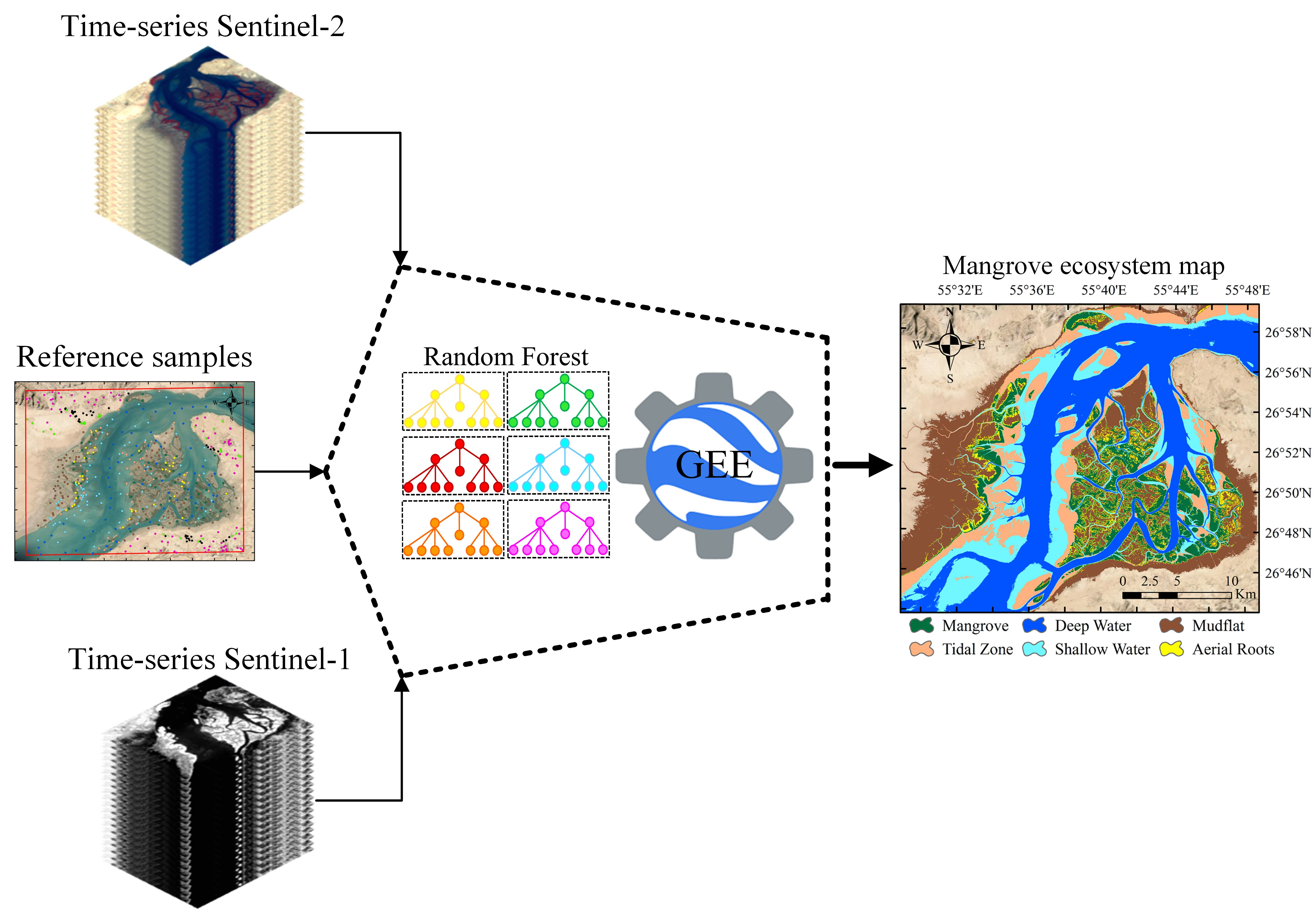
The time-series Sentinel-1 and Sentinel-2 satellite images were integrated to produce an accurate mangrove ecosystem map. Combining SAR and optical data allows the detection of different physical and spectral characteristics of land covers and, thus, their integration may achieve precise classification results [50,51,52]. Additionally, time-series data enables consideration of the water level fluctuations and tidal effects in the mangrove ecosystem, which can also increase the reliability of the classification results [53].
Sentinel-1 is a European SAR satellite, which acquires C-band data in dual-polarization in all-weather conditions with a 6-day temporal resolution. Level-1C ground range detected (GRD) images with 10 m spatial resolution in both ascending and descending modes were employed [54,55]. In total, 86 Sentinel-1 scenes in the VV (vertical transmittance and receiving) and VH (vertical transmittance and horizontal receiving) polarizations, acquired in 2019 (i.e., from 1 January 2019 to 1 January 2020), were employed (see Table 2).
Sentinel-2 is also a European platform launched by the European Space Agency (ESA) and carries the MultiSpectral Instrument (MSI) sensor [54]. This sensor records the Earth’s surface information in 13 spectral bands from visible to shortwave infrared (SWIR) regions, with different spatial resolutions ranging between 10 m and 60 m. In this study, only four bands of blue, green, red, and near infrared (NIR), which are captured with 10 m spatial resolution, were used. As it is acknowledged that satellite imagery with higher spatial resolutions improves mangrove ecosystem mapping, [25], here, only bands with 10 m spatial resolution were employed. This is mainly rooted in the fact that higher spatial resolution imagery improves the delineation of mangrove ecosystem classes, especially identifying mangrove patches with a small area or narrow shapes [56]. In total, 41 Sentinel-2 images, acquired in 2019 (i.e., from 1 January 2019 to 1 January 2020), were considered for mangrove ecosystem mapping (see Table 2).

3. Methodology

The schematic framework, providing an overview of the proposed approach, is presented in Figure 2. This section comprises three sub-sections, in which the satellite data preprocessing, classification workflow, and accuracy assessment procedure are explained in detail.

3.1. Satellite Data Preprocessing

Sentinel-1 GRD data are available within GEE with the snippet of (Image Collection ID: COPERNUCUS/S1_GRD). They are generally ready-to-use data because several preprocessing steps are initially applied to them by the GEE developers. These data are already converted to the backscattering coefficient (σ°, dB) and are ortho-rectified. In particular, five preprocessing steps (1) applying orbit file correction, (2) GRD border noise removal, (3) thermal noise removal, (4) radiometric calibration, and (5) terrain correction were applied to each Sentinel-1 scene, while their detailed information is provided by the GEE developers (https://developers.google.com/earth-engine/guides/sentinel1 accessed on 29 June 2021). Afterward, all available Sentinel-1 scenes in 2019 were categorized based on the seasons of acquisition, followed by applying a mean reducer to generate seasonal time-series data. Downscaling time-series Sentinel-1 data by the mean reducer function produced seasonal datasets, which are less susceptible to image acquisition conditions, and reduced speckle noise [31].
Sentinel-2 top of atmosphere (TOA) reflectance data, which are available within GEE by the snippet (Image Collection ID: COPERNICUS/S2), were also used in this study. The TOA reflectance values were derived through radiometric calibration of raw data. Because of the importance of applying cloud masking, a filtering step was first implemented to remove Sentinel-2 scenes with a cloud cover percentage of higher than 5%. Subsequently, similar to Sentinel-1 data, a seasonal median reducer was applied to all remaining Sentinel-2 scenes, generating seasonal optical features for classification tasks. The median reducer function allows the production of cloud-free seasonal datasets, in which the noisy, very dark, and very bright pixels are also removed [31,57].
Ultimately, eight SAR features (4 VV + 4 VH) and 16 optical features (4 blue + 4 green + 4 red + 4 NIR bands) were used in synergy to produce mangrove ecosystem maps. It is well acknowledged that the quality of the classification results directly depends on the input features [58,59]. As such, the integration of multi-source (i.e., SAR + optical) data can increase the discriminative capability of the classifier [53]. Moreover, time-series satellite data can manifest the water level fluctuations in estuaries, such as mangrove ecosystems [53]. Consequently, seasonal datasets can mitigate the tidal effects in the study area and allow producing cloud-free mosaics.

3.2. Classification

Different classification algorithms have been employed for mangrove mapping using satellite images [23,39,60]. In this regard, choosing the most appropriate classifier, in addition to selecting discriminative features, is important, and directly affects the classification results. Among classifiers, random forest (RF) proved to be an efficient algorithm in mangrove mapping studies [15,44,61]. For instance, Toosi et al. [44] compared four frequently used non-parametric classifiers (i.e., RF, support vector machine (SVM) with linear and radial basis function kernels, and regularized discriminant analysis) for mangrove ecosystem mapping, and concluded that the RF classifier was superior.
RF is an authoritative non-parametric classifier, which employs the bootstrap aggregation technique to combine the classification results of various independent random decision trees and to predict the class label [62]. Each of these random decision trees is trained by a subset of training samples, called in-bag samples, and uses the remnant, called out-of-bag samples, for internal cross-validation. Later, their results are integrated to produce the final classification results. This enables the RF classifier to have a higher tolerance for noise, and also avoids overfitting possibilities [63,64]. Moreover, RF has proven its capability of handling high-dimensional data by resulting in promising maps [31].
In this study, a pixel-based RF classifier was implemented within GEE because of the high potential of the RF classifier for mangrove ecosystem mapping [15,44,61]. In this regard, the final image mosaics, comprising seasonal Sentinel-1 and Sentinel-2 data, were inserted into an RF classifier. Meanwhile, half of the reference samples were employed to train the RF classifier. The RF classifier has several tuning parameters that affect the training phase of the classification step and, thus, directly influence the classification results. Among these parameters, the number of trees and variables at each node are the most influential parameters [63], which were set at 100 and equal to the square root of the number of input features, respectively. It should be noted that these values were determined through several trial and error attempts based on computational efficacy, visual inspection of the classification results, and the average out-of-bag sampling error of the RF classifier in the training phase.

3.3. Accuracy Assessment

Any thematic map derived from remote sensing data should be subjected to a trustworthy accuracy assessment to ensure its quality and reliability [65]. Therefore, both visual interpretation and statistical approaches were conducted to evaluate the accuracy of the final mangrove ecosystem map. High-resolution satellite images available within Google Earth and ArcMap were employed for visual assessment of the classification results. In terms of statistical accuracy assessment, independent test samples were incorporated to generate the confusion matrix, and then other metrics, such as OA, KC, producer accuracy (PA), and user accuracy (UA), were derived. The PA represents how well a specific area can be mapped, whereas the UA is an indicator of how well the produced map represents what really exists in the study area [66]. Furthermore, the F-score, the harmonic average of recall and precision, was computed for each class, and then its macro-averaging was reported for the classification results [67]. As already mentioned in Section 2.2.1, the classification procedure was repeated ten times with different training and test sets to comprehensively assess the classification performance for mangrove ecosystem mapping through a cross-validation step.

4. Results

Figure 3 presents the resulting mangrove ecosystem map (i.e., only classes within the mangrove ecosystem) with 10 m spatial resolution using RF classifier and the integration of seasonal SAR and optical satellite data within GEE. It should be noted that this map was produced based on a majority voting step of ten classification results. The majority voting step allows the production of a more reliable and accurate mangrove ecosystem map [68]. This is rooted in the fact that combining decisions of several classification results can lead to better recognition results [69]. Visually, the thematic map had an acceptable accuracy, indicating the high potential of the proposed method for delineating different classes. Generally, mangrove areas were depicted precisely, and their surroundings were also classified as aerial roots, as these roots grow around mangroves. Furthermore, the middle parts of the tidal channels were correctly classified as deep water, while other parts located near the coastline areas (i.e., tidal zone) were successfully distinguished as shallow water. Additionally, along with their corresponding high-resolution satellite images, two zoomed-in areas are also provided in Figure 3 for better visual interpretation. For instance, Figure 3b,c illustrates a zoomed-in area of the mangrove ecosystem, in which the mangrove areas are successfully identified. Moreover, based on Figure 3d,e, the proposed workflow was highly capable of discriminating between different classes with acceptable precision. In particular, mangrove areas and their surroundings (i.e., aerial roots) were properly discriminated, and also shallow water, deep water, and tidal zone classes were delineated appropriately. Furthermore, other areas without specific covers, which are wet (due to the existence of narrow water channels), were also accurately classified as mudflat.
The consistency images of six classes within the mangrove ecosystem were also computed based on the classification results of ten iterations to determine the robustness of the proposed classification procedure and the consistency of each pixel. It should be noted that the consistency images were produced based on the number of label assignments of each pixel to different classes. In other words, the consistency images present how many times a pixel was assigned to a specific class. The consistency values ranged between one and ten, in which one means very low consistency, while ten means highly consistent. Figure 4 shows the consistency images of six classes within the mangrove ecosystem. It was observed that in almost all cases, the classifier was able to assign consistent labels to each pixel in ten iterations. In particular, mangrove pixels were consistently labeled as mangrove with a high consistency rate of over 85% (i.e., considering pixels with values of eight to ten). Additionally, the tidal zone, deep water, and mudflat classes achieved reasonable rates of stability of over 70%. In contrast, the classes of shallow water and aerial roots obtained lower stability rates. In general, most inconsistencies occurred at boundaries and fragmented locations, where mixed pixels exist, suggesting the necessity of satellite images with a higher spatial resolution for more accurate mapping. For instance, the aerial roots had the highest rate of inconsistency of about 13% (i.e., considering pixels with values of one). This is probably rooted in the fact that these roots grow around mangrove areas and in mudflat conditions, and thus, the classifier may encounter difficulties in distinguishing them. This was more serious in distinguishing aerial roots from mudflat. Furthermore, another source of inconsistency was found between the shallow water and deep water classes, which is in fact associated with their greater similarity. The inconsistency revealed the effect of different training sets and also implied that incorporating the majority voting step could increase the reliability of the final thematic map.
Figure 5 presents the average values of PA and UA along with their standard deviation computed for ten iterations of producing mangrove ecosystem maps. The proposed classification framework obtained high average OA, KC, and F-scores of 93.23% (±1.1), 0.92 (±0.012), and 0.92 (±0.011), respectively. Furthermore, almost all classes achieved high PAs and UAs of over 90%, demonstrating the high potential and applicability of the proposed method for detailed mangrove ecosystem mapping. It is evident that the mangrove classes obtained significant average PA and UA of about 94.4% and 94.5%, indicating the applicability of the implemented approach for accurate mangrove delineation. In fact, the results proved that the proposed approach can not only be used for detailed mangrove ecosystem mapping but also can be effectively employed for accurate mangrove extent mapping. The highest and lowest accuracies were related to deep water and aerial roots, respectively. The aerial roots acquired moderate average PA and UA of approximately 77.6% and 78.2%, respectively, illustrating the challenging task of delineating aerial roots with high accuracy, which is also in accordance with [25]. Furthermore, Figure 5 demonstrates that the proposed approach obtained stable PAs and UAs in all ten iterations, since their standard deviation values ranged between 1.6% and 3.8% for all classes, except for the aerial roots, for which the standard deviation of PAs and UAs were 7.4% and 5.9%, respectively.
The confusion matrices of the classifications were also investigated, to provide an in-depth statistical assessment in each iteration (see Figure 6). Generally, the proposed approach obtained acceptable accuracy since less confusion happened between classes, and confusion matrices were almost diagonal. However, there are several spots where some confusions are observable in Figure 6, such as the confusion between deep water and shallow water, which occurred in all iterations. Additionally, relatively high confusions were also found between aerial roots and other classes of mangrove and mudflat, which were the reasons for the moderate accuracy of aerial roots.
An average confusion matrix (i.e., by averaging and rounding of the corresponding elements in 10 confusion matrices) is also provided in Table 3 to provide a comprehensive overview of all ten confusion matrices at a glance. Table 3 shows that the proposed approach obtained high average OA and KC values of 93.23% and 0.92, respectively, indicating the high potential of this approach for detailed mangrove ecosystem mapping. Moreover, the average omission error (OE) and commission error (CE) values were respectively 7.56% and 7.18%. The dominant confusion was associated with the aerial roots class, causing the highest OE and CE values of 23.06% and 21.92%, respectively, which are also in accordance with [25]. In particular, the two highest confusions occurred interchangeably between aerial roots/mudflat and aerial roots/mangrove. This was because these roots are grown in mudflat areas, exactly around mangroves. Therefore, it was challenging to separate aerial roots from two other classes due to the spectral/backscattering similarities and also the existence of mixed pixels at 10 m spatial resolution. Additionally, the second highest confusion was also observed between deep water and shallow water, which was actually because of their spectral/backscattering similarity.

5. Discussion

5.1. General Findings

Mangrove ecosystems are routinely inundated and are located in inter-tidal zones [21]. Therefore, it is difficult to carry out field surveys to collect reference samples with global positioning system (GPS) devices [15]. The availability of highly accurate reference samples through field surveys is critical for reliable mapping; however, precise visual interpretation of high-resolution satellite images can compensate for this limitation. The proposed method was able to achieve high average OA and KC values, suggesting the suitability of applying this method when conducting fieldwork is difficult. It should be noted that generating reference samples even from high-resolution satellite imagery through precise visual interpretations can cause uncertainties and does not obviate the importance of in situ reference sample collection for more reliable mapping.
Despite the importance of mapping the mangrove extents, which have been conducted more frequently using either traditional or cloud computing-based approaches, fewer studies were devoted to producing detailed mangrove ecosystem maps. However, mapping relevant classes within a mangrove ecosystem (i.e., aerial roots and mudflat) is required to enhance condition assessment and also to suggest appropriate solutions for protection and conservation [25]. In particular, mapping the distribution and condition of aerial roots are highly required for mangrove status monitoring since these roots provide different morphological and physiological adaptions to adverse environmental conditions [70]. For instance, these roots facilitate gas exchange to adapt mangroves to live in oxygen-poor locations [71], protect mangroves from flood effects and hurricanes [70], and mitigate shoreline erosion to prevent mangrove loss [72]. Furthermore, these roots support mangrove growth and accretion by stabilizing mudflat conditions [71,73]. Therefore, obtaining precise information about aerial roots helps to conduct more profound monitoring of mangroves and also to determine the locations for efficient reforestation programs.
In this study, the GEE cloud computing platform was employed for mangrove ecosystem mapping. GEE provides an unprecedented opportunity to employ dense time-series data from free-of-charge satellite images, and also it contains many built-in machine learning and image processing algorithms for satellite data manipulations [29,30]. Furthermore, the existence of ready-to-use data, along with other characteristics, contributes towards developing efficient methods with higher rates of automation and, thus, decreases the dedicated time for data acquisition, calibrating, and preprocessing [26]. Despite these advantages, GEE also has several limitations, such as restrictions on using numerous features and training samples (i.e., encountering limit exceed), which were also addressed in previous studies [32].

5.2. Comparison with the Latest Global Mangrove Maps

The obtained results indicated the high applicability of the proposed method for mangrove ecosystem mapping and also mangrove extent delineation. Therefore, the mangrove extent derived from the proposed method was compared with the recent available global mangrove extent map [74]. This global mangrove map was produced at 25 m (0.8 arc-second) spatial resolution using multi-source remote sensing data of the Advanced Land Observation Satellite (ALOS) Phased-Array L-band SAR (PALSAR) and optical data of Landsat-5 and Landsat-7 through an Extremely Randomized Trees (ERT) classifier [74]. Figure 7 presents the mangrove extent resultants of two products, along with the corresponding high-resolution satellite images for better visualization. Based on Figure 7, it is obvious that the proposed approach outperformed the global mangrove product. Clearly, based on Figure 7a–c, the proposed method was resistant to misclassification, probably of mudflat and aerial roots (i.e., generally unvegetated areas between mangrove patches). Likewise, Figure 7d–f also illustrates that the proposed method was successful at delineating narrow mangrove patches which occurred along the tidal zone areas. Despite the subtle differences in the classification algorithms and the considered classes in each workflow, the main discrepancies between the two maps were almost associated with the spatial resolution of remote sensing satellite data, which suggests the use of Sentinel-1 and Sentinel-2 data. Therefore, the synergistic use of Sentinel-1 and Sentinel-2 can definitely enhance the recent global mangrove extent mapping [53]. Although the utility of 10 m spatial resolution indeed enhanced the mangrove extent mapping, as the results suggest, it is still necessary to use satellite images with a higher spatial resolution to permit the production of more precise detailed mangrove ecosystem maps. This is rooted in the fact that higher spatial resolutions are necessary to discriminate between different classes that are located near each other, and to reduce the mixed pixel effect, such as separating aerial roots from two other classes of mangrove and mudflat. However, the current high cost of acquiring commercial high-resolution images is the main limiting factor.

5.3. Contribution of Multi-Source Remote Sensing Data

As mentioned earlier, the Sentinel-1 SAR and Sentinel-2 optical data were combined to produce an accurate mangrove ecosystem map. It has been well acknowledged that a combination of optical and SAR remote sensing data could enhance the classification results of land cover mapping [75]. However, few studies have combined optical and SAR data for detailed mangrove ecosystem mapping, and they were mainly conducted based on optical data [25,76]. Therefore, here, the contribution of multi-source remote sensing data for detailed mangrove ecosystem mapping was evaluated based on two metrics of OA and KC. In this regard, the explained workflow (Section 3) was repeated with two other scenarios of using only optical or SAR data. The obtained results for the multi-source data processing were comprehensively discussed in the previous section, and the average OA and KC were 93.23% and 0.92, respectively. The average OA and KC achieved for the scenario, in which only optical data were incorporated, were 90.67% and 0.89, respectively. Although the accuracies based on the optical data were still satisfactory, the decline in the accuracies indicates the contribution of multi-source remote sensing data for more accurate mangrove ecosystem mapping. In particular, the use of only optical data resulted in over 1.5% (i.e., averaged over ten iterations) loss of class accuracies of each tidal zone, deep water, shallow water, and mudflat classes. Additionally, the results using only SAR data revealed a weak performance (i.e., OA = 62.98% and KC = 0.58); however, the SAR data was successful at delineating mangrove areas with a high accuracy of over 90% in almost all iterations. When using only SAR data, the lower accuracy was mainly associated with the low capability of separating different classes (i.e., except mangrove) within the mangrove ecosystem, with an average loss of 31.94% in class accuracies. The obtained results suggest that the inclusion of SAR data in the classification task, along with optical data, leads to producing a precise and accurate mangrove ecosystem map. This is mainly due to the fact that these two data sources can provide complementary information about the spectral and physical properties of different classes [77,78].

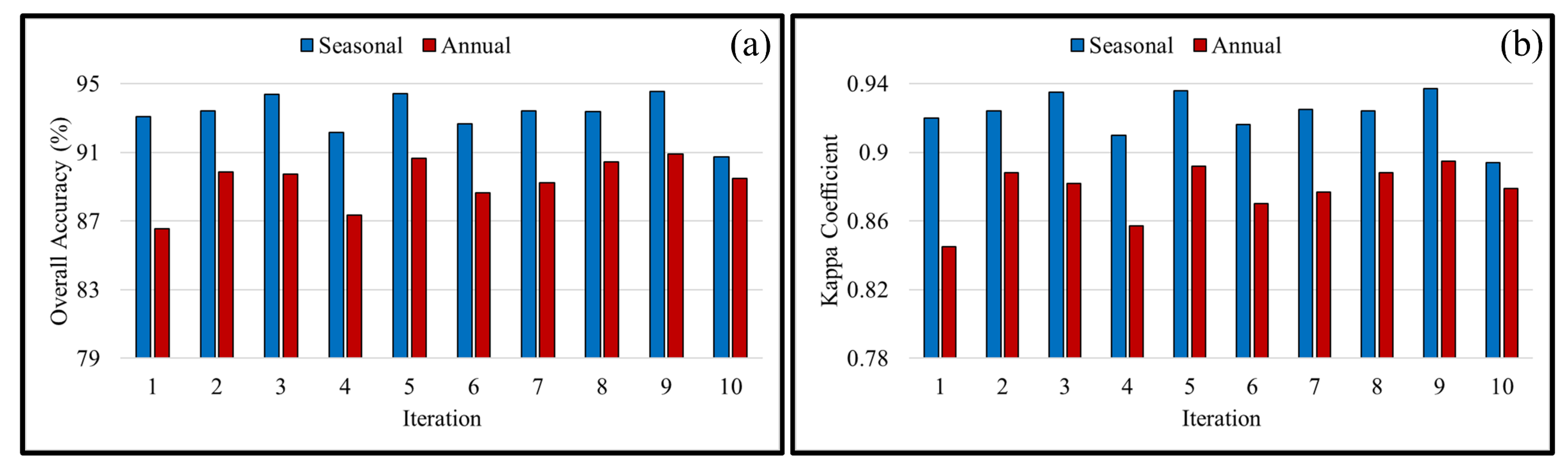
5.4. Comparison with Annual Downscaling

The seasonal downscaling approach was implemented for mangrove ecosystem mapping. In fact, the dense time-series SAR and optical data, acquired in 2019, were downscaled to seasonal features for further analysis. This approach takes the benefits of multi-temporal image analysis, as well as reducing the computational complexity of considering all available images without downscaling. Furthermore, since the mangrove ecosystems are routinely located in the inter-tidal zone and are inundated [21], the classifier may be influenced by the inundation intensity [79], biasing the mangrove extent and area. One solution is to use a single date image, in which the lowest tidal condition occurred; however, finding an image with such criteria may be challenging for several reasons, such as the presence of cloud and low temporal resolution of satellites. Therefore, it is recommended to apply time-series data to acquire more reliable classification results. In this study, seasonal features were used; however, other researchers applied annual downscaling for mangrove mapping [39]. Consequently, the usefulness of seasonal downscaling is compared with the annual downscaling approach. In this regard, the mentioned workflow was also applied to annual downscaled SAR and optical data, and the obtained results were compared with the seasonal approach. As is clear from Figure 8, incorporating seasonal downscaling achieved higher OAs and KCs in all iterations and, thus, it suggests that the seasonal downscaling can provide more discriminative information compared to annual downscaling [80]. This may be rooted in the fact that annual downscaling would override the tidal fluctuations, while the seasonal downscaling includes seasonal variations of water level (i.e., dry and wet seasons), reflecting tidal fluctuations [78].

6. Conclusions

Producing detailed mangrove ecosystem maps is essential for natural resource monitoring and sustainable development goals tracking. In this paper, a straightforward yet robust workflow was proposed to produce mangrove ecosystem maps with high accuracies. For this purpose, Sentinel-1 and Sentinel-2 data were inserted into an RF classifier within the GEE cloud computing platform. The final classification results were comprehensively evaluated through different analyses, and further discussions were provided. The classification results obtained high average OA and KC of 93.23% and 0.92, respectively. Moreover, all the classes obtained high accuracies, except the aerial roots, which achieved moderate accuracies in all cases, suggesting the consideration of other possible solutions (i.e., higher resolution images) for more accurate delineation of this class. Altogether, taking both qualitative (i.e., visual interpretation) and quantitative (i.e., statistical accuracy assessment) evaluation criteria into account, the proposed method confirmed its applicability in producing a detailed mangrove ecosystem map. Furthermore, the comparison results proved the contribution of multi-source remote sensing data (i.e., SAR + optical), as well as the effectiveness of seasonal downscaling. The proposed workflow was implemented based on an open-source platform and free-of-charge satellite data, making it appealing and applicable in almost all countries.

Author Contributions

Conceptualization, A.G. and S.Z.; methodology, A.G. and S.Z.; software, A.G.; validation, A.G., S.Z. and R.M.A.; formal analysis, A.G.; investigation, A.G.; data curation, A.G. and S.Z.; writing—original draft preparation, A.G. and R.M.A.; writing—review and editing, A.G., S.Z., R.M.A., M.A., S.J., A.M.; visualization, A.G.; supervision, A.G., A.M. and S.J.; project administration, A.G.; funding acquisition, M.A. and S.J. All authors have read and agreed to the published version of the manuscript.

Funding

S.J. was partially funded by Knut and Alice Wallenberg grant 99007-RFh2018-2016.

Data Availability Statement

The produced mangrove ecosystem map using Sentinel-1, Sentinel-2, and Random Forest algorithm and the derived mangrove extent map are available upon request from the first author.

Acknowledgments

The authors would like to thank the European Space Agency (ESA) to freely provide Sentinel-1 and Sentinel-2 satellite data. Additionally, the authors thank the anonymous three reviewers for their comments.

Conflicts of Interest

The authors declare no conflict of interest.

References

  1. Chai, M.; Li, R.; Shi, C.; Shen, X.; Li, R.; Zan, Q. Contamination of polybrominated diphenyl ethers (PBDEs) in urban mangroves of Southern China. Sci. Total Environ. 2019, 646, 390–399. [Google Scholar] [CrossRef]
  2. Veettil, B.K.; Pereira, S.F.R.; Quang, N.X. Rapidly diminishing mangrove forests in Myanmar (Burma): A review. Hydrobiologia 2018, 822, 19–35. [Google Scholar] [CrossRef]
  3. Doughty, C.L.; Langley, J.A.; Walker, W.S.; Feller, I.C.; Schaub, R.; Chapman, S.K. Mangrove range expansion rapidly increases coastal wetland carbon storage. Estuar. Coasts 2016, 39, 385–396. [Google Scholar] [CrossRef]
  4. Debrot, A.O.; Veldhuizen, A.; Van Den Burg, S.W.K.; Klapwijk, C.J.; Islam, M.; Alam, M.; Ahsan, M.; Ahmed, M.U.; Hasan, S.R.; Fadilah, R.; et al. Non-Timber Forest Product Livelihood-Focused Interventions in Support of Mangrove Restoration: A Call to Action. Forests 2020, 11, 1224. [Google Scholar] [CrossRef]
  5. Giri, C.; Ochieng, E.; Tieszen, L.L.; Zhu, Z.; Singh, A.; Loveland, T.; Masek, J.; Duke, N. Status and distribution of mangrove forests of the world using earth observation satellite data. Glob. Ecol. Biogeogr. 2011, 20, 154–159. [Google Scholar] [CrossRef]
  6. Bhargava, R.; Sarkar, D.; Friess, D.A. A cloud computing-based approach to mapping mangrove erosion and progradation: Case studies from the Sundarbans and French Guiana. Estuar. Coast. Shelf Sci. 2020. [Google Scholar] [CrossRef]
  7. Mafi-Gholami, D.; Jaafari, A.; Zenner, E.K.; Kamari, A.N.; Bui, D.T. Spatial modeling of exposure of mangrove ecosystems to multiple environmental hazards. Sci. Total Environ. 2020, 740. [Google Scholar] [CrossRef] [PubMed]
  8. Chen, B.; Xiao, X.; Li, X.; Pan, L.; Doughty, R.; Ma, J.; Dong, J.; Qin, Y.; Zhao, B.; Wu, Z.; et al. A mangrove forest map of China in 2015: Analysis of time series Landsat 7/8 and Sentinel-1A imagery in Google Earth Engine cloud computing platform. ISPRS J. Photogramm. Remote Sens. 2017, 131, 104–120. [Google Scholar] [CrossRef]
  9. Romañach, S.S.; DeAngelis, D.L.; Koh, H.L.; Li, Y.; Teh, S.Y.; Barizan, R.S.R.; Zhai, L. Conservation and restoration of mangroves: Global status, perspectives, and prognosis. Ocean. Coast. Manag. 2018, 154, 72–82. [Google Scholar] [CrossRef]
  10. Primavera, J.H. Mangroves, fishponds, and the quest for sustainability. Science 2005, 310, 57–59. [Google Scholar] [CrossRef] [Green Version]
  11. Duncan, C.; Owen, H.J.F.; Thompson, J.R.; Koldewey, H.J.; Primavera, J.H.; Pettorelli, N. Satellite remote sensing to monitor mangrove forest resilience and resistance to sea level rise. Methods Ecol. Evol. 2018, 9, 1837–1852. [Google Scholar] [CrossRef] [Green Version]
  12. Lovelock, C.E.; Cahoon, D.R.; Friess, D.A.; Guntenspergen, G.R.; Krauss, K.W.; Reef, R.; Rogers, K.; Saunders, M.L.; Sidik, F.; Swales, A.; et al. The vulnerability of Indo-Pacific mangrove forests to sea-level rise. Nature 2015, 526, 559–563. [Google Scholar] [CrossRef] [PubMed] [Green Version]
  13. Mafi-Gholami, D.; Zenner, E.K.; Jaafari, A. Mangrove regional feedback to sea level rise and drought intensity at the end of the 21st century. Ecol. Indic. 2020, 110. [Google Scholar] [CrossRef]
  14. Jaramillo, F.; Desormeaux, A.; Hedlund, J.; Jawitz, J.W.; Clerici, N.; Piemontese, L.; Rodríguez-Rodriguez, J.A.; Anaya, J.A.; Blanco-Libreros, J.F.; Borja, S.; et al. Priorities and interactions of sustainable development goals (SDGs) with focus on wetlands. Water 2019, 11, 619. [Google Scholar] [CrossRef] [Green Version]
  15. Zhao, C.; Qin, C.-Z. 10-m-resolution mangrove maps of China derived from multi-source and multi-temporal satellite observations. ISPRS J. Photogramm. Remote Sens. 2020, 169, 389–405. [Google Scholar] [CrossRef]
  16. Kuenzer, C.; Bluemel, A.; Gebhardt, S.; Quoc, T.V.; Dech, S. Remote sensing of mangrove ecosystems: A review. Remote Sens. 2011, 3, 878–928. [Google Scholar] [CrossRef] [Green Version]
  17. Wicaksono, P.; Danoedoro, P.; Hartono; Nehren, U. Mangrove biomass carbon stock mapping of the Karimunjawa Islands using multispectral remote sensing. Int. J. Remote Sens. 2016, 37, 26–52. [Google Scholar] [CrossRef]
  18. Giri, C.; Long, J. Is the geographic range of mangrove forests in the conterminous United States really expanding? Sensors 2016, 16, 2010. [Google Scholar] [CrossRef] [PubMed] [Green Version]
  19. Hauser, L.T.; An Binh, N.; Viet Hoa, P.; Hong Quan, N.; Timmermans, J. Gap-Free Monitoring of Annual Mangrove Forest Dynamics in Ca Mau Province, Vietnamese Mekong Delta, Using the Landsat-7-8 Archives and Post-Classification Temporal Optimization. Remote Sens. 2020, 12, 3729. [Google Scholar] [CrossRef]
  20. Cao, J.; Leng, W.; Liu, K.; Liu, L.; He, Z.; Zhu, Y. Object-based mangrove species classification using unmanned aerial vehicle hyperspectral images and digital surface models. Remote Sens. 2018, 10, 89. [Google Scholar] [CrossRef] [Green Version]
  21. Zhu, X.; Hou, Y.; Weng, Q.; Chen, L. Integrating UAV optical imagery and LiDAR data for assessing the spatial relationship between mangrove and inundation across a subtropical estuarine wetland. ISPRS J. Photogramm. Remote Sens. 2019, 149, 146–156. [Google Scholar] [CrossRef]
  22. Abdel-Hamid, A.; Dubovyk, O.; El-Magd, A.; Menz, G. Mapping mangroves extents on the Red Sea coastline in Egypt using polarimetric SAR and high resolution optical remote sensing data. Sustainability 2018, 10, 646. [Google Scholar] [CrossRef] [Green Version]
  23. Manna, S.; Raychaudhuri, B. Mapping distribution of Sundarban mangroves using Sentinel-2 data and new spectral metric for detecting their health condition. Geocarto Int. 2020, 35, 434–452. [Google Scholar] [CrossRef]
  24. Kabiri, K. Mapping coastal ecosystems and features using a low-cost standard drone: Case study, Nayband Bay, Persian gulf, Iran. J. Coast. Conserv. 2020, 24, 1–8. [Google Scholar] [CrossRef]
  25. Bihamta Toosi, N.; Soffianian, A.R.; Fakheran, S.; Pourmanafi, S.; Ginzler, C.; Waser, L.T. Land Cover Classification in Mangrove Ecosystems Based on VHR Satellite Data and Machine Learning—An Upscaling Approach. Remote Sens. 2020, 12, 2684. [Google Scholar] [CrossRef]
  26. Cárdenas, N.Y.; Joyce, K.E.; Maier, S.W. Monitoring mangrove forests: Are we taking full advantage of technology? Int. J. Appl. Earth Obs. Geoinf. 2017, 63, 1–14. [Google Scholar] [CrossRef] [Green Version]
  27. Giri, C.; Pengra, B.; Long, J.; Loveland, T.R. Next generation of global land cover characterization, mapping, and monitoring. Int. J. Appl. Earth Obs. Geoinf. 2013, 25, 30–37. [Google Scholar] [CrossRef]
  28. Giri, C. Observation and monitoring of mangrove forests using remote sensing: Opportunities and challenges. Remote Sens. 2016, 8, 783. [Google Scholar] [CrossRef] [Green Version]
  29. Gorelick, N.; Hancher, M.; Dixon, M.; Ilyushchenko, S.; Thau, D.; Moore, R. Google Earth Engine: Planetary-scale geospatial analysis for everyone. Remote Sens. Environ. 2017, 202, 18–27. [Google Scholar] [CrossRef]
  30. Amani, M.; Ghorbanian, A.; Ahmadi, S.A.; Kakooei, M.; Moghimi, A.; Mirmazloumi, S.M.; Moghaddam, S.H.A.; Mahdavi, S.; Ghahremanloo, M.; Parsian, S.; et al. Google Earth Engine Cloud Computing Platform for Remote Sensing Big Data Applications: A Comprehensive Review. IEEE J. Sel. Top. Appl. Earth Obs. Remote Sens. 2020, 13, 5326–5350. [Google Scholar] [CrossRef]
  31. Ghorbanian, A.; Kakooei, M.; Amani, M.; Mahdavi, S.; Mohammadzadeh, A.; Hasanlou, M. Improved land cover map of Iran using Sentinel imagery within Google Earth Engine and a novel automatic workflow for land cover classification using migrated training samples. ISPRS J. Photogramm. Remote Sens. 2020, 167, 276–288. [Google Scholar] [CrossRef]
  32. Amani, M.; Mahdavi, S.; Afshar, M.; Brisco, B.; Huang, W.; Mohammad Javad Mirzadeh, S.; White, L.; Banks, S.; Montgomery, J.; Hopkinson, C. Canadian wetland inventory using google earth engine: The first map and preliminary results. Remote Sens. 2019, 11, 842. [Google Scholar] [CrossRef] [Green Version]
  33. Zhang, M.; Huang, H.; Li, Z.; Hackman, K.O.; Liu, C.; Andriamiarisoa, R.L.; Ny Aina Nomenjanahary Raherivelo, T.; Li, Y.; Gong, P. Automatic High-Resolution Land Cover Production in Madagascar Using Sentinel-2 Time Series, Tile-Based Image Classification and Google Earth Engine. Remote Sens. 2020, 12, 3663. [Google Scholar] [CrossRef]
  34. Genzano, N.; Pergola, N.; Marchese, F. A Google Earth Engine tool to investigate, map and monitor volcanic thermal anomalies at global scale by means of mid-high spatial resolution satellite data. Remote Sens. 2020, 12, 3232. [Google Scholar] [CrossRef]
  35. Cao, B.; Domke, G.M.; Russell, M.B.; Walters, B.F. Spatial modeling of litter and soil carbon stocks on forest land in the conterminous United States. Sci. Total Environ. 2019, 654, 94–106. [Google Scholar] [CrossRef] [PubMed]
  36. Pérez-Romero, J.; Navarro-Cerrillo, R.M.; Palacios-Rodriguez, G.; Acosta, C.; Mesas-Carrascosa, F.J. Improvement of remote sensing-based assessment of defoliation of Pinus spp. caused by Thaumetopoea Pityocampa Denis and Schiffermüller and related environmental drivers in Southeastern Spain. Remote Sens. 2019, 11, 1736. [Google Scholar] [CrossRef] [Green Version]
  37. Seydi, S.T.; Akhoondzadeh, M.; Amani, M.; Mahdavi, S. Wildfire Damage Assessment over Australia Using Sentinel-2 Imagery and MODIS Land Cover Product within the Google Earth Engine Cloud Platform. Remote Sens. 2021, 13, 220. [Google Scholar] [CrossRef]
  38. Beselly, S.M.; van der Wegen, M.; Grueters, U.; Reyns, J.; Dijkstra, J.; Roelvink, D. Eleven Years of Mangrove--Mudflat Dynamics on the Mud Volcano-Induced Prograding Delta in East Java, Indonesia: Integrating UAV and Satellite Imagery. Remote Sens. 2021, 13, 1084. [Google Scholar] [CrossRef]
  39. Mondal, P.; Liu, X.; Fatoyinbo, T.E.; Lagomasino, D. Evaluating Combinations of Sentinel-2 Data and Machine-Learning Algorithms for Mangrove Mapping in West Africa. Remote Sens. 2019, 11, 2928. [Google Scholar] [CrossRef] [Green Version]
  40. Baloloy, A.B.; Blanco, A.C.; Ana, R.R.C.S.; Nadaoka, K. Development and application of a new mangrove vegetation index (MVI) for rapid and accurate mangrove mapping. ISPRS J. Photogramm. Remote Sens. 2020, 166, 95–117. [Google Scholar] [CrossRef]
  41. Yancho, J.M.M.; Jones, T.G.; Gandhi, S.R.; Ferster, C.; Lin, A.; Glass, L. The Google Earth Engine Mangrove Mapping Methodology (GEEMMM). Remote Sens. 2020, 12, 3758. [Google Scholar] [CrossRef]
  42. Milani, A.S. Mangrove forests of the Persian Gulf and the Gulf of Oman. In Threats to Mangrove Forests; Springer: Berlin/Heidelberg, Germany, 2018; pp. 53–75. [Google Scholar]
  43. Milani, S.A.; Beglu, J.M. Satellite based assessment of the area and changes in the Mangrove ecosystem of the QESHM island, Iran. J. Environ. Res. Dev. 2012, 7, 1052–1060. [Google Scholar]
  44. Toosi, N.B.; Soffianian, A.R.; Fakheran, S.; Pourmanafi, S.; Ginzler, C.; Waser, L.T. Comparing different classification algorithms for monitoring mangrove cover changes in southern Iran. Glob. Ecol. Conserv. 2019, 19, e00662. [Google Scholar] [CrossRef]
  45. Hajializadeh, P.; Safaie, M.; Naderloo, R.; Shojaei, M.G.; Gammal, J.; Villnäs, A.; Norkko, A. Species Composition and Functional Traits of Macrofauna in Different Mangrove Habitats in the Persian Gulf. Front. Mar. Sci. 2020, 7, 809. [Google Scholar] [CrossRef]
  46. Dadashi, M.; Ghaffari, S.; Bakhtiari, A.R.; Tauler, R. Multivariate curve resolution of organic pollution patterns in mangrove forest sediment from Qeshm Island and Khamir Port—Persian Gulf, Iran. Environ. Sci. Pollut. Res. 2018, 25, 723–735. [Google Scholar] [CrossRef]
  47. Lohr, S.L. Sampling: Design and Analysis; CRC Press: Bocaton, FL, USA, 2019. [Google Scholar]
  48. Mahdianpari, M.; Jafarzadeh, H.; Granger, J.E.; Mohammadimanesh, F.; Brisco, B.; Salehi, B.; Homayouni, S.; Weng, Q. A large-scale change monitoring of wetlands using time series Landsat imagery on Google Earth Engine: A case study in Newfoundland. GIScience Remote Sens. 2020, 57, 1102–1124. [Google Scholar] [CrossRef]
  49. Geiß, C.; Pelizari, P.A.; Schrade, H.; Brenning, A.; Taubenböck, H. On the effect of spatially non-disjoint training and test samples on estimated model generalization capabilities in supervised classification with spatial features. IEEE Geosci. Remote Sens. Lett. 2017, 14, 2008–2012. [Google Scholar]
  50. Dong, D.; Wang, C.; Yan, J.; He, Q.; Zeng, J.; Wei, Z. Combing Sentinel-1 and Sentinel-2 image time series for invasive Spartina alterniflora mapping on Google Earth Engine: A case study in Zhangjiang Estuary. J. Appl. Remote Sens. 2020, 14, 44504. [Google Scholar] [CrossRef]
  51. Mahdavi, S.; Salehi, B.; Amani, M.; Granger, J.; Brisco, B.; Huang, W. A dynamic classification scheme for mapping spectrally similar classes: Application to wetland classification. Int. J. Appl. Earth Obs. Geoinf. 2019, 83. [Google Scholar] [CrossRef]
  52. Xia, J.; Yokoya, N.; Pham, T.D. Probabilistic mangrove species mapping with multiple-source remote-sensing datasets using label distribution learning in Xuan Thuy National Park, Vietnam. Remote Sens. 2020, 12, 3834. [Google Scholar] [CrossRef]
  53. Wang, L.; Jia, M.; Yin, D.; Tian, J. A review of remote sensing for mangrove forests: 1956–2018. Remote Sens. Environ. 2019, 231. [Google Scholar] [CrossRef]
  54. Malenovsky, Z.; Rott, H.; Cihlar, J.; Schaepman, M.E.; Garcia-Santos, G.; Fernandes, R.; Berger, M. Sentinels for science: Potential of Sentinel-1,-2, and-3 missions for scientific observations of ocean, cryosphere, and land. Remote Sens. Environ. 2012, 120, 91–101. [Google Scholar] [CrossRef]
  55. Torres, R.; Snoeij, P.; Geudtner, D.; Bibby, D.; Davidson, M.; Attema, E.; Potin, P.; Rommen, B.; Floury, N.; Brown, M.; et al. GMES Sentinel-1 mission. Remote Sens. Environ. 2012, 120, 9–24. [Google Scholar] [CrossRef]
  56. Liu, X.; Fatoyinbo, T.E.; Thomas, N.M.; Guan, W.W.; Zhan, Y.; Mondal, P.; Lagomasino, D.; Simard, M.; Trettin, C.C.; Deo, R.; et al. Large-scale High-resolution Coastal Mangrove Forests Mapping across West Africa with Machine Learning Ensemble and Satellite Big Data. Front. Earth Sci. 2021, 8, 677. [Google Scholar] [CrossRef]
  57. Naboureh, A.; Li, A.; Bian, J.; Lei, G.; Amani, M. A Hybrid Data Balancing Method for Classification of Imbalanced Training Data within Google Earth Engine: Case Studies from Mountainous Regions. Remote Sens. 2020, 12, 3301. [Google Scholar] [CrossRef]
  58. Ghorbanian, A.; Mohammadzadeh, A. An unsupervised feature extraction method based on band correlation clustering for hyperspectral image classification using limited training samples. Remote Sens. Lett. 2018. [Google Scholar] [CrossRef]
  59. Ghorbanian, A.; Maghsoudi, Y.; Mohammadzadeh, A. Clustering-Based Band Selection Using Structural Similarity Index and Entropy for Hyperspectral Image Classification Clustering-Based Band Selection Using Structural Similarity Index and Entropy for Hyperspectral Image Classification. Trait. Signal. 2020, 37, 785–791. [Google Scholar] [CrossRef]
  60. Quang, N.H.; Quinn, C.H.; Stringer, L.C.; Carrie, R.; Hackney, C.R.; Van Hue, L.T.; Van Tan, D.; Nga, P.T.T. Multi-Decadal Changes in Mangrove Extent, Age and Species in the Red River Estuaries of Viet Nam. Remote Sens. 2020, 12, 2289. [Google Scholar] [CrossRef]
  61. Nababa, I.I.; Symeonakis, E.; Koukoulas, S.; Higginbottom, T.P.; Cavan, G.; Marsden, S. Land Cover Dynamics and Mangrove Degradation in the Niger Delta Region. Remote Sens. 2020, 12, 3619. [Google Scholar] [CrossRef]
  62. Breiman, L. Random forests. Mach. Learn. 2001, 45, 5–32. [Google Scholar] [CrossRef] [Green Version]
  63. Belgiu, M.; Dragut, L. Random forest in remote sensing: A review of applications and future directions. ISPRS J. Photogramm. Remote Sens. 2016, 114, 24–31. [Google Scholar] [CrossRef]
  64. Morell-Monzó, S.; Sebastiá-Frasquet, M.-T.; Estornell, J. Land Use Classification of VHR Images for Mapping Small-Sized Abandoned Citrus Plots by Using Spectral and Textural Information. Remote Sens. 2021, 13, 681. [Google Scholar] [CrossRef]
  65. Stehman, S. V Sampling designs for accuracy assessment of land cover. Int. J. Remote Sens. 2009, 30, 5243–5272. [Google Scholar] [CrossRef]
  66. Story, M.; Congalton, R.G. Accuracy assessment: A user’s perspective. Photogramm. Eng. Remote Sens. 1986, 52, 397–399. [Google Scholar]
  67. Berger, A.; Guda, S. Threshold optimization for F measure of macro-averaged precision and recall. Pattern Recognit. 2020, 102. [Google Scholar] [CrossRef]
  68. Ruta, D.; Gabrys, B. Classifier selection for majority voting. Inf. Fusion 2005, 6, 63–81. [Google Scholar] [CrossRef]
  69. Amani, M.; Salehi, B.; Mahdavi, S.; Brisco, B.; Shehata, M. A Multiple Classifier System to improve mapping complex land covers: A case study of wetland classification using SAR data in Newfoundland, Canada. Int. J. Remote Sens. 2018, 39, 7370–7383. [Google Scholar] [CrossRef]
  70. Srikanth, S.; Lum, S.K.Y.; Chen, Z. Mangrove root: Adaptations and ecological importance. Trees 2016, 30, 451–465. [Google Scholar] [CrossRef]
  71. Al-Khayat, J.A.; Alatalo, J.M. Relationship Between Tree Size, Sediment Mud Content, Oxygen Levels, and Pneumatophore Abundance in the Mangrove Tree Species Avicennia Marina (Forssk.) Vierh. J. Mar. Sci. Eng. 2021, 9, 100. [Google Scholar] [CrossRef]
  72. Duke, N.C.; Kovacs, J.M.; Griffiths, A.D.; Preece, L.; Hill, D.J.E.; Van Oosterzee, P.; Mackenzie, J.; Morning, H.S.; Burrows, D. Large-scale dieback of mangroves in Australia’s Gulf of Carpentaria: A severe ecosystem response, coincidental with an unusually extreme weather event. Mar. Freshw. Res. 2017, 68, 1816–1829. [Google Scholar] [CrossRef]
  73. Okello, J.A.; Kairo, J.G.; Dahdouh-Guebas, F.; Beeckman, H.; Koedam, N. Mangrove trees survive partial sediment burial by developing new roots and adapting their root, branch and stem anatomy. Trees 2020, 34, 37–49. [Google Scholar] [CrossRef] [Green Version]
  74. Bunting, P.; Rosenqvist, A.; Lucas, R.M.; Rebelo, L.-M.; Hilarides, L.; Thomas, N.; Hardy, A.; Itoh, T.; Shimada, M.; Finlayson, C.M. The global mangrove watch—A new 2010 global baseline of mangrove extent. Remote Sens. 2018, 10, 1669. [Google Scholar] [CrossRef] [Green Version]
  75. Amani, M.; Salehi, B.; Mahdavi, S.; Granger, J.; Brisco, B. Wetland classification in Newfoundland and Labrador using multi-source SAR and optical data integration. GIScience Remote Sens. 2017, 54, 779–796. [Google Scholar] [CrossRef]
  76. Wang, D.; Wan, B.; Qiu, P.; Su, Y.; Guo, Q.; Wang, R.; Sun, F.; Wu, X. Evaluating the performance of sentinel-2, landsat 8 and pléiades-1 in mapping mangrove extent and species. Remote Sens. 2018, 10, 1468. [Google Scholar] [CrossRef] [Green Version]
  77. Chauhan, S.; Srivastava, H.S. Comparative evaluation of the sensitivity of multi-polarized SAR and optical data for various land cover classes. Int. J. Adv. Remote Sens. GIS Geogr. 2016, 4, 1–14. [Google Scholar]
  78. Zhao, C.; Qin, C.-Z.; Teng, J. Mapping large-area tidal flats without the dependence on tidal elevations: A case study of Southern China. ISPRS J. Photogramm. Remote Sens. 2020, 159, 256–270. [Google Scholar] [CrossRef]
  79. Wang, X.; Xiao, X.; Zou, Z.; Hou, L.; Qin, Y.; Dong, J.; Doughty, R.B.; Chen, B.; Zhang, X.; Chen, Y.; et al. Mapping coastal wetlands of China using time series Landsat images in 2018 and Google Earth Engine. ISPRS J. Photogramm. Remote Sens. 2020, 163, 312–326. [Google Scholar] [CrossRef]
  80. Wang, L.; Silván-Cárdenas, J.L.; Sousa, W.P. Neural network classification of mangrove species from multi-seasonal Ikonos imagery. Photogramm. Eng. Remote Sens. 2008, 74, 921–927. [Google Scholar] [CrossRef]
Figure 1. The geographical extent of the Hara protected area of Qeshm Island in southern Iran, along with the spatial distribution of reference samples over the study area (reference samples information is provided in Table 1).
Remotesensing 13 02565 g001
Figure 2. Framework of the proposed method for mangrove ecosystem mapping using the random forest (RF) algorithm and a combination of the Sentinel-1 and Sentinel-2 satellite images within the Google Earth Engine (GEE) platform.
Remotesensing 13 02565 g002
Figure 3. Mangrove ecosystem map of the study area produced using the random forest (RF) algorithm and a combination of the Sentinel-1 and Sentinel-2 satellite images within the Google Earth Engine (GEE) platform (a), two zoomed areas of the produced map (b,d), and their corresponding high-resolution satellite images for better visualization (c,e).
Remotesensing 13 02565 g003
Figure 4. Consistency images of six classes (a) mangrove, (b) tidal zone, (c) deep water, (d) shallow water, (e) mudflat, and (f) aerial roots in the mangrove ecosystem. The consistency values ranged between one and ten, indicating very low and very high consistency, respectively.
Remotesensing 13 02565 g004
Figure 5. Average producer accuracy (PA) and user accuracy (UA) of different classes along with their standard deviation (black error bars) computed from ten iterations.
Remotesensing 13 02565 g005
Figure 6. Confusion matrices of mangrove ecosystem maps for ten iterations.
Remotesensing 13 02565 g006
Figure 7. High-resolution satellite images of two mangrove areas (a,d), mangrove extents from the recent global mangrove map (b,e) [74], and mangrove extents derived from the proposed method (c,f).
Remotesensing 13 02565 g007
Figure 8. Overall accuracy (OA; (a)) and Kappa coefficient (KC; (b)) of annual and seasonal downscaling of SAR and optical data for mangrove ecosystem mapping.
Remotesensing 13 02565 g008
Table 1. The number and area of training and test polygons for nine classes that were considered in this study.
IDClassTraining SamplesTest SamplesTotal
PolygonArea (ha)PolygonArea (ha)PolygonArea (ha)
1Mangrove2414.592715.305139.89
2Tidal zone3017.042213.385230.42
3Deep water2917.673623.126540.79
4Shallow water4416.313515.677931.98
5Mudflat4319.234320.818640.04
6Aerial roots2010.01209.054019.06
7Urban187.65249.824217.47
8Bare ground4017.614118.418136.20
9Vegetation175.11164.82339.93
Total265125.22264130.38529529
Table 2. The number of Sentinel-1 and Sentinel-2 satellite images in each season.
DataSeasonTotalDate
SpringSummerAutumnWinter
Sentinel-12222222086From 1 January 2019 to 1 January 2020
Sentinel-2111112741
Table 3. Average confusion matrix of mangrove ecosystem mapping using the random forest (RF) algorithm and a combination of the Sentinel-1 and Sentinel-2 satellite images processed within the Google Earth Engine (GEE) platform.
MangroveTidal ZoneDeep WaterShallow WaterMudflatAerial RootsUrbanBare GroundVegetation
Mangrove1582000075000
Tidal Zone01613072310000
Deep Water0022356000000
Shallow Water046108164500000
Mudflat000020911402200
Aerial Roots94000152823002
Urban000090923486
Bare Ground0000706019643
Vegetation2000416144518
PA (%)95.4793.9997.3891.4492.8176.9494.4796.5692.83
UA (%)94.2797.2295.3992.5791.5178.0890.5797.4298.29
OE (%)4.536.012.628.567.1923.065.533.447.17
CE (%)5.732.784.617.438.4921.929.432.581.71
Overall Accuracy (OA) = 93.23%Kappa Coefficient (KC) = 0.92
Publisher’s Note: MDPI stays neutral with regard to jurisdictional claims in published maps and institutional affiliations.

