An Adaptive Capsule Network for Hyperspectral Remote Sensing Classification

Abstract

The capsule network (Caps) is a novel type of neural network that has great potential for the classification of hyperspectral remote sensing. However, the Caps suffers from the issue of gradient vanishing. To solve this problem, a powered activation regularization based adaptive capsule network (PAR-ACaps) was proposed for hyperspectral remote sensing classification, in which an adaptive routing algorithm without iteration was applied to amplify the gradient, and the powered activation regularization method was used to learn the sparser and more discriminative representation. The classification performance of PAR-ACaps was evaluated using two public hyperspectral remote sensing datasets, i.e., the Pavia University (PU) and Salinas (SA) datasets. The average overall classification accuracy (OA) of PAR-ACaps with shallower architecture was measured and compared with those of the benchmarks, including random forest (RF), support vector machine (SVM), 1-dimensional convolutional neural network (1DCNN), two-dimensional convolutional neural network (CNN), three-dimensional convolutional neural network (3DCNN), Caps, and the original adaptive capsule network (ACaps) with comparable network architectures. The OA of PAR-ACaps for PU and SA datasets was 99.51% and 94.52%, respectively, which was higher than those of benchmarks. Moreover, the classification performance of PAR-ACaps with relatively deeper neural architecture (four and six convolutional layers in the feature extraction stage) was also evaluated to demonstrate the effectiveness of gradient amplification. As shown in the experimental results, the classification performance of PAR-ACaps with relatively deeper neural architecture for PU and SA datasets was also superior to 1DCNN, CNN, 3DCNN, Caps, and ACaps with comparable neural architectures. Additionally, the training time consumed by PAR-ACaps was significantly lower than that of Caps. The proposed PAR-ACaps is, therefore, recommended as an effective alternative for hyperspectral remote sensing classification.

1. Introduction

Land use is essential to global climate change, urban planning, and management [1]. With the appearance of remote sensing, large-scale land-use mapping has become practicable and economical. However, it is difficult to extract accurate land use from low- and medium-resolution remotely sensed imagery. With the development of imaging technology, remote sensing images with fine spatial resolution (FSR), such as RapidEye, IKONOS, WorldView, and uninhabited aerial vehicle synthetic aperture radar images, have been widely used in the field of urban land-use information extraction. However, many FSR images consist of four bands. The low spectral resolution leads to overlaps among the reflected signals of different ground objects, and then many land-use types cannot be distinguished in detail.

The hyperspectral remotely sensed image (HSI) captures the ground objects’ spectral signals with hundreds of narrow bands and provides abundant spectral information [2]. Simultaneously, the spatial information (e.g., textures) provided by HSI becomes more detailed with the improvement of spatial resolution [3]. Therefore, the information provided by HSI is sufficient for the extraction of detailed land-use information. However, the massive bands often lead to the curse of dimensionality [4]. The classification performances of the commonly used classifiers (e.g., support vector machine (SVM) and random forest (RF)) for HSI were often limited without the reduction of feature dimensionality (e.g., feature extraction and feature selection).

Deep learning (DL) has been a significant research breakthrough in the field of artificial intelligence in recent years. Inspired by human vision, it introduces hierarchical structure to extract and learn features for completing various tasks [5]. In recent years, DL has yielded promising performance in many fields [6]. Deep convolutional neural network (CNN) is a representative “end to end” feature-learning algorithm in the field of DL. Due to its outperformance and robustness, CNN has been widely used in diverse fields such as object recognition, image classification, and speech recognition [7]. In the field of remote sensing, CNN has also been widely used for the accurate classification of crop, urban land use, wetland, and so on [8,9,10,11]. For the classification of hyperspectral remote sensing, CNN-based methods including 1D, 2D, 3D-CNN, multiscale CNN, residual CNN, and object-based CNN have been proposed [12,13,14,15]. However, CNN failed in learning the spatial hierarchies between features and lost some spatial information (e.g., location) in the pooling layer. Thus, the performance of CNN remains to be improved [16].

Sabour et al. [17] proposed a novel type of neural network called capsule network (Caps) (Figure 1). Caps stacks the features of the feature map into vectors, namely capsules. The orientation and the overall length of the capsule represent the properties and the existence of entity, respectively. The relationship between the partial and the whole is obtained by updating the coupling coefficient between the low-layer capsule and the high-layer capsule through the dynamic routing algorithm [18]. So far, the outperformance of Caps has been demonstrated in many fields such as image segmentation, object recognition, and action detection [19,20,21,22]. In the field of remote sensing, Caps was initially used for the classification of hyperspectral remote sensing, and its performance is superior to that of CNN [23,24,25].

Although Caps has better performance on some datasets, the robustness of Caps is limited for the classification of complex datasets. One of the most important reasons is gradient vanishing caused by the sparsity of coupling coefficient [18]. To improve the distribution of the values of the coupling coefficients, some normalization techniques, such as Max-Min and sigmoid, were used to obtain better performance on complex datasets [26,27]. To further improve the performance of Caps, the capsule network with k-means was proposed [28]. However, these modified routing algorithms could not effectively speed up the training process due to the inner loop. Thus, the number of parameters of Caps cannot be reduced effectively. What is worse, the depth of the Caps is thus limited; namely, only a few convolutional layers can be used to extract the features from HSI. Thus, high-level semantic features are absent in the Caps.

To overcome the shortcomings of Caps, an adaptive routing algorithm is presented in [18]. In this routing algorithm, the gradient coefficient $\gamma$, instead of coupling coefficient $c_{ij}$, is used to amplify the gradient. Thus, the capsule network based on adaptive routing algorithm (ACaps) can stack multiple convolution layers for high-level semantic feature extraction because the amplified gradient can be better transmitted to the layers in the front of the model. However, the performance of the ACaps for complex dataset (CIFAR10) is also far from satisfactory. An important reason for the poor performance of capsule network on complex datasets is that the original squash function encourages the capsules with low energies to have large activation values [29]. This leads to an unreasonable higher distribution of activation values. Thus, many capsules encode irrelevant information which causes disturbance and then leads to poor performance.

With the inspiration of the adaptive routing algorithm, a kind of hyperspectral remote sensing classification method based on ACaps was proposed. Unlike the original ACaps, the powered activation regularization (PAR) method was proposed to repress the strength of connections of capsules in adjacent capsule layers. PAR can force the net to learn a sparser and more discriminative representation to improve the classification performance. For the convenience of expression, the classification method is called PAR-ACaps. The performance of the proposed classifier with shallow architecture was compared with those of the benchmarks, including SVM, RF, 1DCNN, CNN, 3DCNN, Caps, and ACaps. Likewise, the effectiveness of PAR-ACaps with relatively deeper architecture was also demonstrated.

The rest of the paper is organized as follows: Section 2 presents the HSI datasets and introduces the Caps and the proposed PAR-ACaps in detail. The experimental results are provided in Section 3, followed by a discussion in Section 4. The conclusions are drawn in Section 5.

2. Materials and Methods

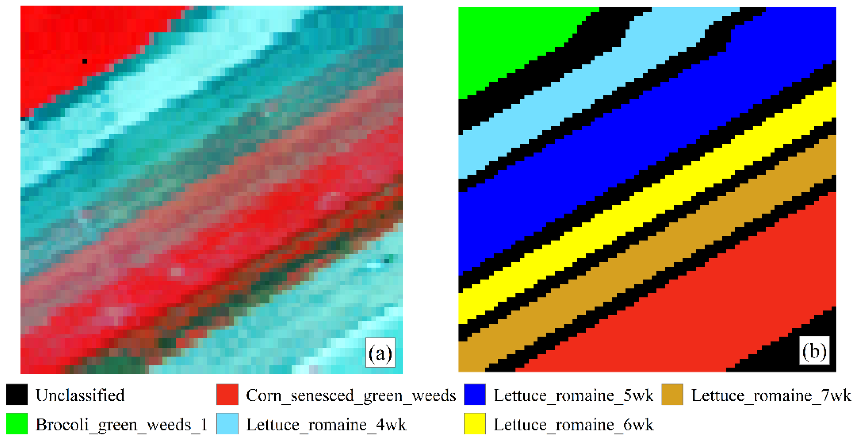
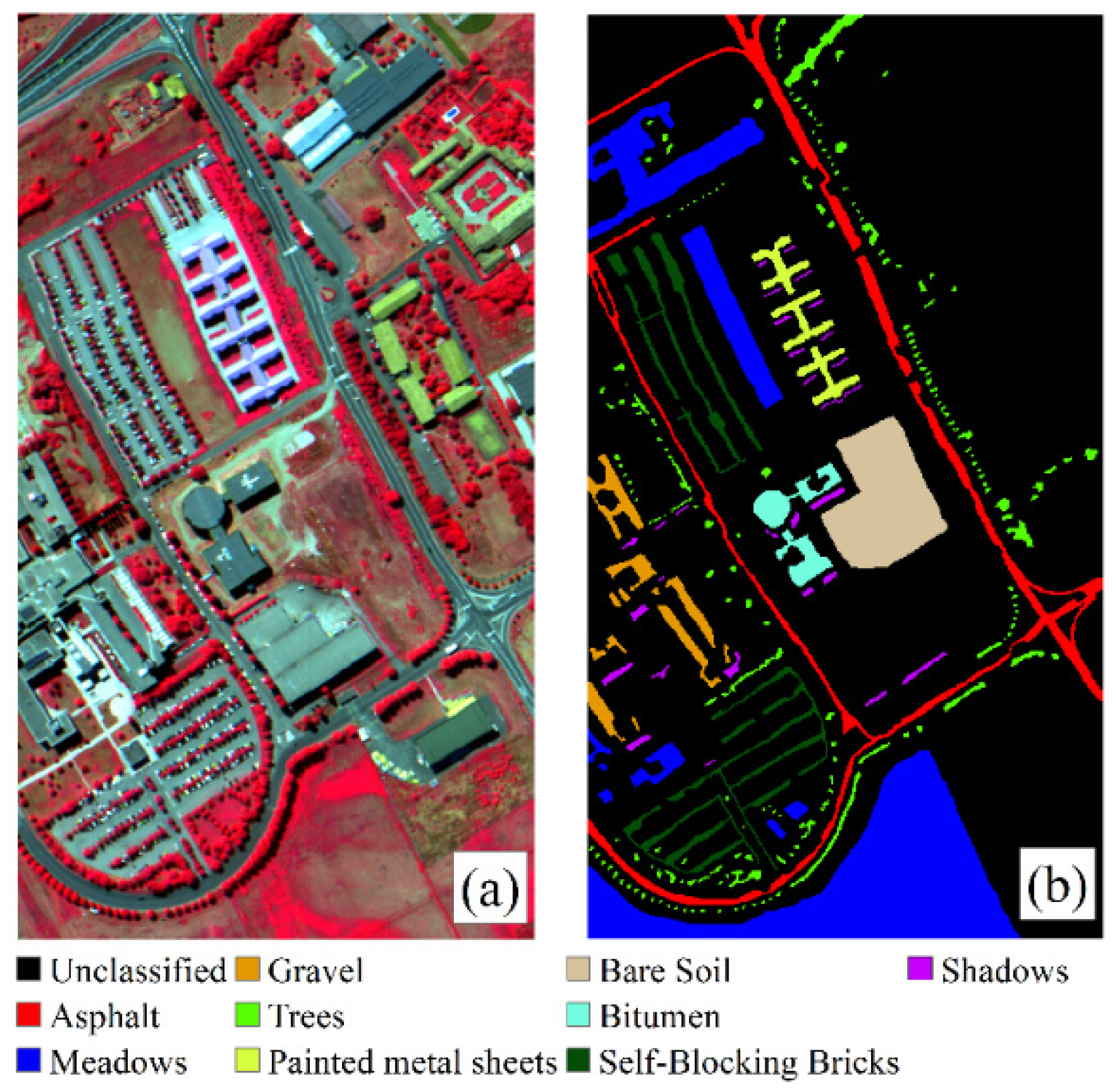
2.1. Data Source

In our experiment, two public hyperspectral datasets were employed to test the performance of the proposed PAR-ACaps, including Salinas-A and Pavia University datasets.

Salinas-A dataset (SA dataset): The data were acquired by AVIRIS sensor over the Salinas Valley, California (Figure 2a). The dataset consists of 224 bands over a spectrum range of 400–2500 nm. It has a spatial extent of 86 × 63 pixels with a spatial resolution of 3.7 m. A total of 204 bands were reserved after discarding the bands (i.e., 108–112, 154–167, and 224) that were adversely influenced by moisture absorption. There were 6 land-use/cover types in the ground truth (Figure 2b), including Brocoli_green_weeds_1, Corn_senesced_green_weeds, Lettuce_romaine_4wk, Lettuce_romaine_5wk, Lettuce_romaine_6wk, and Lettuce_romaine_7wk. The number of training, validation, and testing samples for each of the 6 classes collected from the ground truth map is shown in

Table 1. The number of samples for the PU and SA dataset.

Dataset	Class No.	Land Cover/Use Type	Number of Samples
			Training	Validation	Test	Total
SA	1	Brocoli_green_weeds_1	100	100	191	391
	2	Corn_senesced_green_weeds	390	390	563	1343
	3	Lettuce_romaine_4wk	150	150	316	616
	4	Lettuce_romaine_5wk	470	470	585	1525
	5	Lettuce_romaine_6wk	210	210	254	674
	6	Lettuce_romaine_7wk	250	250	299	799
PU	1	Asphalt	1000	1000	4631	6631
	2	Meadows	1000	1001	16,650	18,651
	3	Gravel	460	461	1180	2101
	4	Trees	890	891	1285	3066
	5	Painted metal sheets	400	401	546	1347
	6	Bare Soil	1000	1001	3030	5031
	7	Bitumen	400	401	531	1332
	8	Self-Blocking Bricks	1000	1001	1683	3684
	9	Shadows	260	261	428	949

.

Pavia University dataset (PU dataset): The original PU dataset, acquired by the reflective optics system imaging spectrometer (ROSIS) sensor, consists of 115 bands in the spectral region of 430–860 nm. The dataset has a spatial resolution of 1.3 m with a spatial extent of 610 × 340 pixels (Figure 3a). The bands influenced by water absorption were removed, and there were 103 bands remaining in the dataset. In total, nine land-use/cover types were identified (Figure 3b), including Asphalt, Meadows, Gravel, Trees, Painted metal sheets, Bare Soil, Bitumen, Self-Blocking Bricks, and Shadows. The number of training, validation, and testing samples of each class collected from the ground truth map is also shown in Table 1.

2.2. Method

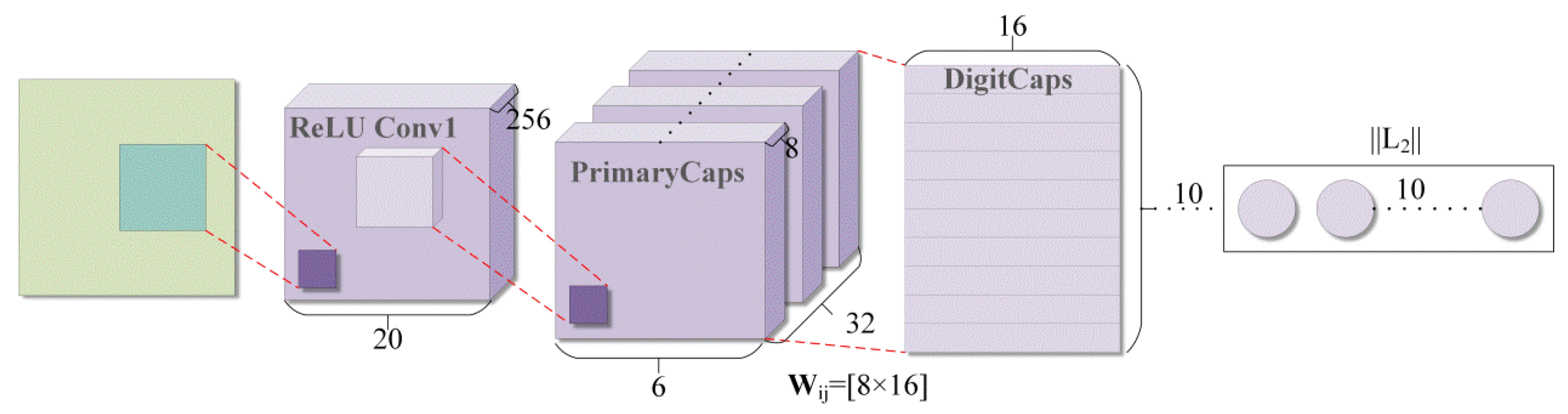
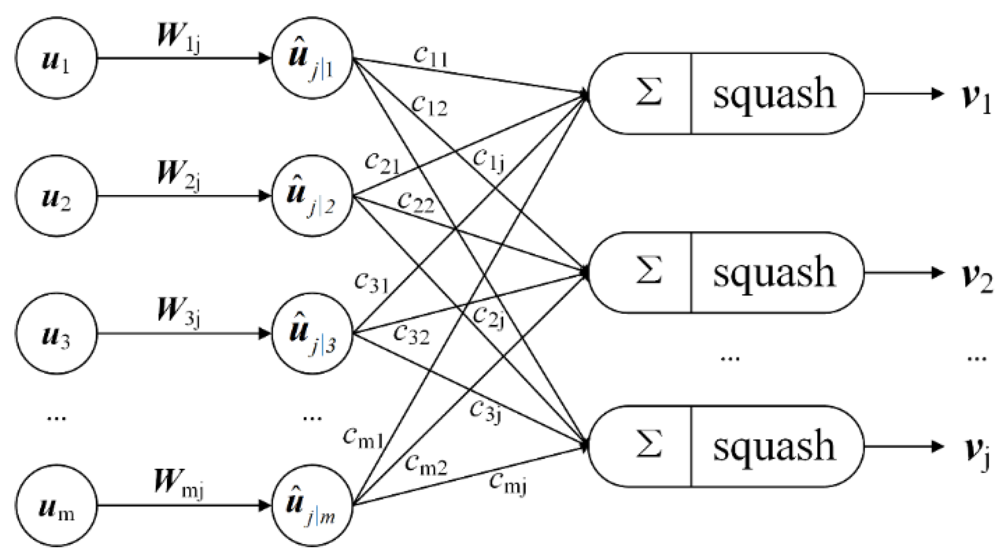
2.2.1. Overview of Capsule Network

Caps is more robust than CNN for the affine transformation of target classification, and the number of needed training samples is fewer. Capsule is defined as a group of hidden neurons. It is a vector whose direction and length represent the entity’s attribute and the probability of entity existence, respectively [17]. The Caps presented by Sabour et al. (2017) consisted of input layer, output layer, convolutional layer, primary capsule (PrimaryCaps) layer, dynamic routing algorithm (Algorithm 1), and digital capsule (DigitCaps) layer (Figure 1). Herein, the convolutional layer is used to extract the low-level features of the classification target. The PrimaryCaps layer captures the spatial relationships among the features by using the capsules. The low-level features encoded by PrimaryCaps layer are transferred to DigitCaps and are predicted using dynamic routing agreement [30]. Specifically, the dynamic routing algorithm adjusts the value of coupling coefficients according to the similarity between the low-layer capsule and the corresponding high-layer capsule, i.e., the higher the similarity is, the bigger the coupling coefficient between them. With the iteration process, the ${\hat{u}}_{j|i}$, obtained by affine transformation of capsule $u_i$ (Equation (1)), moves toward the corresponding high-layer capsule when the similarity between them is higher (Equation (2)).

$${\hat{u}}_{j|i}=W_{ij}{u}_i$$

(1)

$$s_j={\displaystyle \sum }_i{c}_{ij}{\hat{u}}_{j|i}$$

(2)

where $W$ represents the weight matrix that indicates the spatial relationship among the features. $s_j$ is the total input of capsule j. The coupling coefficient $c_{ij}$ between capsule i and all capsules in the high layer sum to 1 and can be calculated by using the “softmax” function as follows:

$$c_{ij}=\frac{\exp \left(b_{ij}\right)}{{\sum }_k\exp \left(b_{ik}\right)}$$

(3)

where logits $b_{ij}$ are the prior probabilities that capsule i should be coupled to capsule j in the high layer. $b_{ij}$ is initialized as 0.

The output of the capsule in the (l + 1)-th layer is defined as $v_j$; the length of $v_j$ is compressed to [0, 1) by using a nonlinear “squashing” function (Equation (4)).

$$v_j=\frac{{\Vert s_j\Vert }^2}{1+{\Vert s_j\Vert }^2}\frac{s_j}{\Vert s_j\Vert }$$

(4)

The whole computational process between the capsule layers is illustrated in Figure 4.

Algorithm 1: Dynamic routing algorithm.

1: procedure Routing (${\hat{u}}_{j|i}$, r, l) 2:   for every capsule i in layer l and capsule j in layer (l+1): $b_{ij}\leftarrow 0$. 3:   for r iterations do 4:     for every capsule i in layer l: $c_i\leftarrow \mathrm{softmax}\left(b_i\right)$ 5:     for every capsule j in layer (l+1): $s_j\leftarrow \sum _i{c}_{ij}{\hat{u}}_{j|i}$ 6:     for every capsule j in layer (l+1): $v_j\leftarrow \mathrm{squash}\left(s_j\right)$ 7:     for every capsule i in layer l and capsule j in layer (l+1):$b_{ij}\leftarrow b_{ij}+{\hat{u}}_{j|i}·v_j$ 8:   return $v_j$

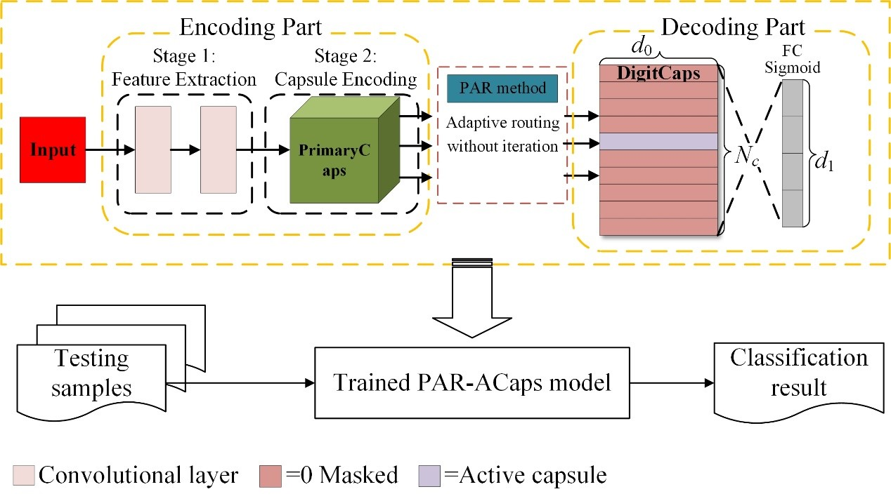
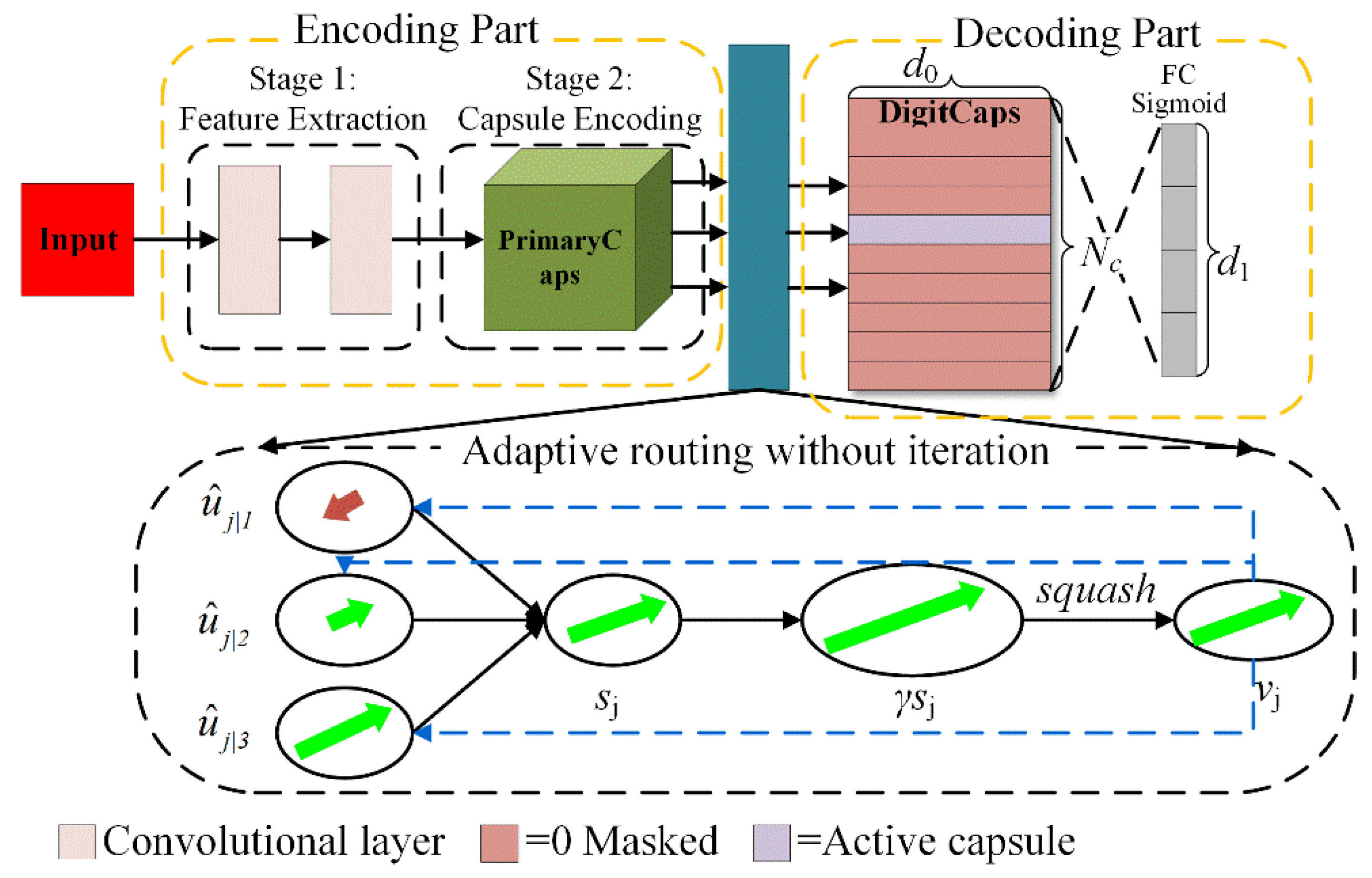
2.2.2. PAR-Based Adaptive Capsule Network

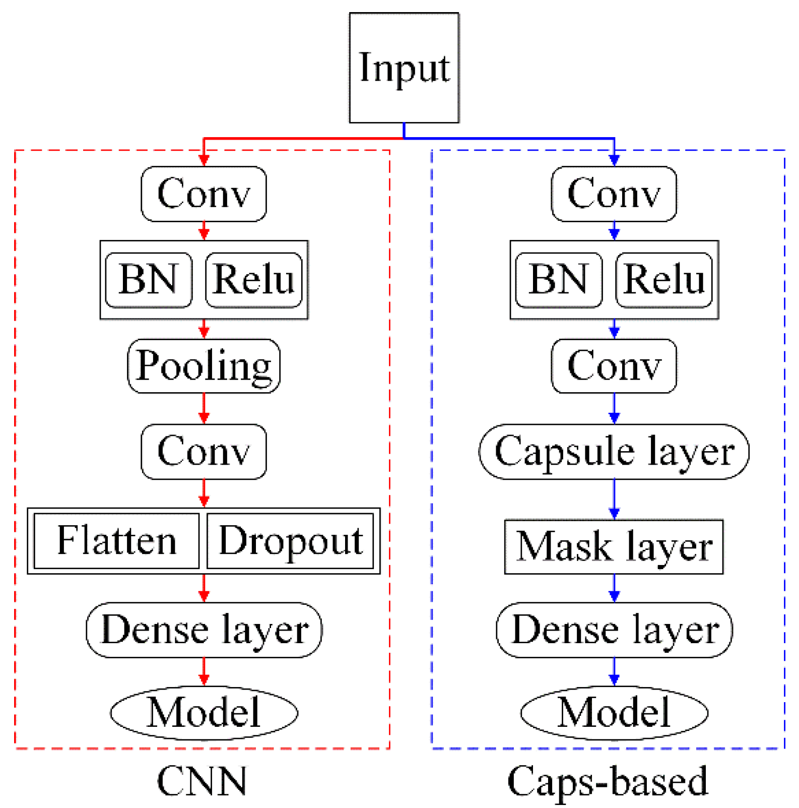
• The architecture of ACaps

Similar to the architecture of Caps, the ACaps consists of feature extraction, capsule encoding units, and decoder units. The features extracted by convolutional layers are sent to the primary capsule layer and then encoded as capsules. The output of the last capsule layer encodes the instantiation parameters of the input image with the encourage of reconstruction loss (Equation (5)). After that, the image reconstruction is implemented by using the decoder structure which consists of a stack of fully connected layers (Figure 5). In the decoder structure, all but the activity vector of the correct image capsule is masked, and then the activity vector is used to reconstruct the input image. The difference between the reconstructed image and the original input image is measured by Euclidean distance and minimized during the training process.

$$L_k=T_k max{\left(0, m^{+}-\Vert v_k\Vert \right)}^2+\lambda \left(1-T_k\right) \max {\left(0, \Vert v_k\Vert -m^{-}\right)}^2$$

(5)

where $T_k=1$ and $\Vert v_k\Vert$ represent k-th target labels and the length of k-th digit capsule, respectively. $m^{+}=0.9$ and $m^{-}=0.1$ denote the minimum margin and the maximum margin, respectively. $\lambda =0.5$ is the downweighting factor for preventing the Caps-based methods from shrinking into the local optimum.

• Adaptive routing algorithm without iteration

As mentioned above, the low-layer capsules with the coupling coefficient $c_{ij}$ is learned to obtain the relationship between the partial features and the whole through a dynamic routing algorithm. However, $c_{ij}$ shows a large sparsity after several iterations of training [18]. This causes the gradient vanishing and the ineffectiveness of capsule network when stacking multiple layers. To avoid the gradient vanishing when stacking multiple layers, a kind of adaptive routing algorithm is presented in [18]. In the adaptive routing algorithm, the new ${\hat{u}}_{j|i}$ of low-layer capsule always moves toward the corresponding high-layer capsule despite the degree of similarity between them. As a result, the directionality of the original ${\hat{u}}_{j|i}$ is adaptively enhanced when the similarity is higher and reduced when the similarity is lower. In this paper, the adaptive update process of ${\hat{u}}_{j|i}$ is defined as follows:

$${\hat{u}}_{j|i}={\hat{u}}_{j|i}+v_j$$

(6)

Because there is no parameter to be trained in the routing process and only the capsules in the lower layer are summed, the number of iterations of the adaptive routing algorithm is set to 1, and the iteration process in the adaptive routing algorithm is removed. The pseudocode of the adaptive routing algorithm without iteration is shown in Algorithm 2. The adaptive routing algorithm without iteration introduces the gradient coefficient $\gamma$ amplifies the gradient and removes the iteration process to improve the computational efficiency. The output $v_j$ of the capsule j in layer (l + 1) can be calculated as follows:

$$v_j=\mathrm{squash}({\displaystyle \sum }_i\gamma {\hat{u}}_{j|i})$$

(7)

where squash() is a nonlinear squash function which is elaborated in detail in what follows.

• PAR method

The activation value of a capsule represents the probability that a specific type of object or object part exists, whereas the squash function of ACaps encourages the capsules with low energy to have large activation values. Thus, the irrelevant information cannot be filtered out and may be then entangled with the effective information. It is disadvantageous to the ACaps to make a good decision from the information it receives. To learn the more discriminative presentation and improve the classification performance of the ACaps, the PAR method was proposed and defined as follows:

$$v_j={\Vert s_j\Vert }^n\frac{s_j}{\Vert s_j\Vert }$$

(8)

where $n$ is a hyperparameter, and it was set to 2 in this paper. The power squash function can improve the computation of the likelihood that an entity representing an object’s feature exists from the length of the capsule.

The algorithm for the adaptive routing without iteration for hyperspectral remote sensing classification is shown in Algorithm 2.

Algorithm 2: Adaptive routing without iteration.

1: procedure Routing (${\hat{u}}_{j|i}$, r, l) 2:   capsule i in layer l and capsule j in layer (l+1) 3:   $s_j\leftarrow \sum _i{\hat{u}}_{j|i}$ 4:   $v_j\leftarrow \mathrm{squash}\left(\gamma s_j\right)$ 5:   ${\hat{u}}_{j|i}\leftarrow v_j+{\hat{u}}_{j|i}$ 6:   return $v_j$ 7: end procedure

The calculation process of the adaptive routing algorithm without iteration is also illustrated in Figure 5. The direction of the corresponding capsule $v_j$ in the higher layer is the same as that of the longer capsule in the lower layer through the adaptive routing process. The features encoded by the low-layer capsule are thus clustered, and the corresponding capsule in the higher layer has a higher probability of being activated. Conversely, other capsules with lower probabilities in the higher layers are masked and excluded from the image reconstruction process by using the masking method presented in [16].

3. Results

3.1. Experimental Settings

To validate the effectiveness of the PAR-ACaps, the classification performances of the proposed method tested on SA and PU datasets were compared with those of the benchmarks, including 1DCNN, CNN, 3DCNN, Caps, ACaps, RF, and SVM with radial basis function kernel. For a fair comparison between CNN and Caps-based classifiers, the network architectures are designed as similarly as possible to suppress the diversity. Because the deep neural network may lead to vanishing gradient and result in inferior classification performance, these architectures shown in Figure 6 are relatively shallower, smaller neural networks. In the CNN and Caps-based models, there are two convolutional layers for feature extraction. The kernel size was set to 3 × 3 for the convolutional layer with a stride of 1. The number of filters in each convolutional layer was set to 128. The maximum pooling layer with 2 × 2 filter was employed in the CNN model. These models were trained on a laptop equipped with an Intel Core i7-9700 3.00 GHz processor and 16 GB of memory.

For convincing comparisons between the classification performances of PAR-ACaps and those of benchmarks, the quantitative comparisons of the classification accuracies of those models were necessary, which have typically been achieved using popular hypothesis testing approaches based on tests of the statistical significance of the difference or inequality in the values observed [31]. McNemar’s test has been widely adopted in remote sensing classification as a tool for evaluating the significance of a difference in accuracy. The improvements of PAR-ACaps in classification performances relative to benchmarks were thus analyzed using McNemar’s test.

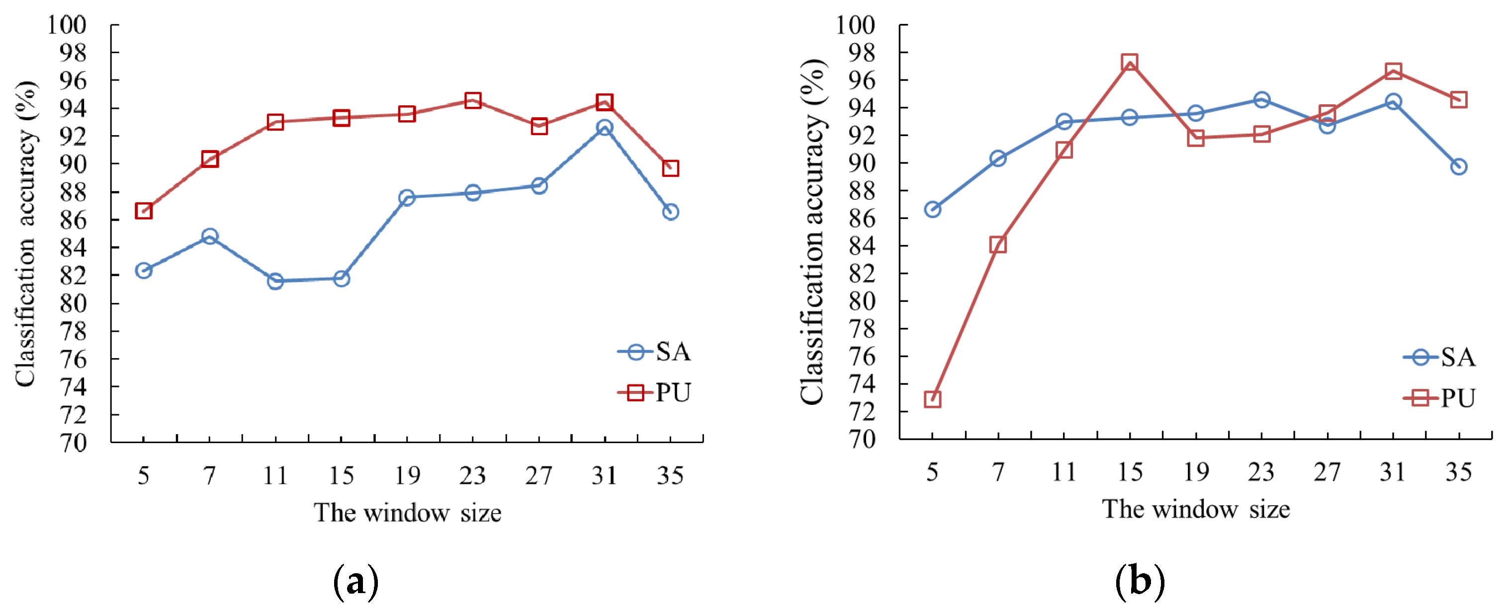
3.1.1. The Effect of the Window Size

The input window size has an important influence on the classification performances of the CNN and Caps-based models. To obtain the optimized input window size, these models were trained on the SA and PU datasets with differently sized inputs. For the CNN and Caps, the input sizes were 5 × 5, 7 × 7, 11 × 11, 15 × 15, 19 × 19, 23 × 23, 27 × 27, 31 × 31, and 35 × 35. The training processes with each size of input window were repeated 5 times, and the average overall classification accuracies (OA) were obtained to evaluate the classification performances.

As shown in Figure 7, the average OAs of CNN achieved the maximum when the input window sizes for PU and SA datasets were 31 × 31. In the following experiments, the input window sizes of CNN for PU and SA datasets were thus set to 31 × 31. For the Caps, the maximum OA (97.29%) for PU dataset was achieved with the input window size of 15 × 15. Meanwhile, the secondary maximum OA (96.66%) of Caps, approximate with the highest, was obtained by using the input images with the size of 31 × 31. When performed on the SA dataset, Caps achieved the highest average OA (94.44%) with the input window size of 31 × 31. Because the window size has significant effect on the computational efficiency of Caps, the window size of Caps for both PU and SA datasets was set to 31 × 31 for a fair comparison.

3.1.2. The Effect of Gradient Coefficient $\mathsf{\gamma }$

As mentioned above, the gradient coefficient $\gamma$ has the effectiveness of amplifying the gradient and improving the computational efficiency of PAR-ACaps. Thus, a sensitivity analysis was conducted to further investigate the effect of the different values of $\gamma$ on the overall classification accuracy of ACaps-based classification method (

Table 2. The effect of the hyperparameter $\gamma$ on the overall classification accuracy (%).

	$\mathit{\gamma }=1$	$\mathit{\gamma }=2$	$\mathit{\gamma }=3$	$\mathit{\gamma }=4$
PU	98.50	99.06	99.16	98.70
SA	88.22	88.81	95.41	80.25

). The classification performances of PAR-ACaps in terms of OA were validated on both PU and SA datasets for the cases of $\gamma =$1, 2, 3, and 4. As shown in Table 2, the highest OAs can be obtained for the case of $\gamma =3$ when tested with both PU and SA datasets.

3.2. Classification Result

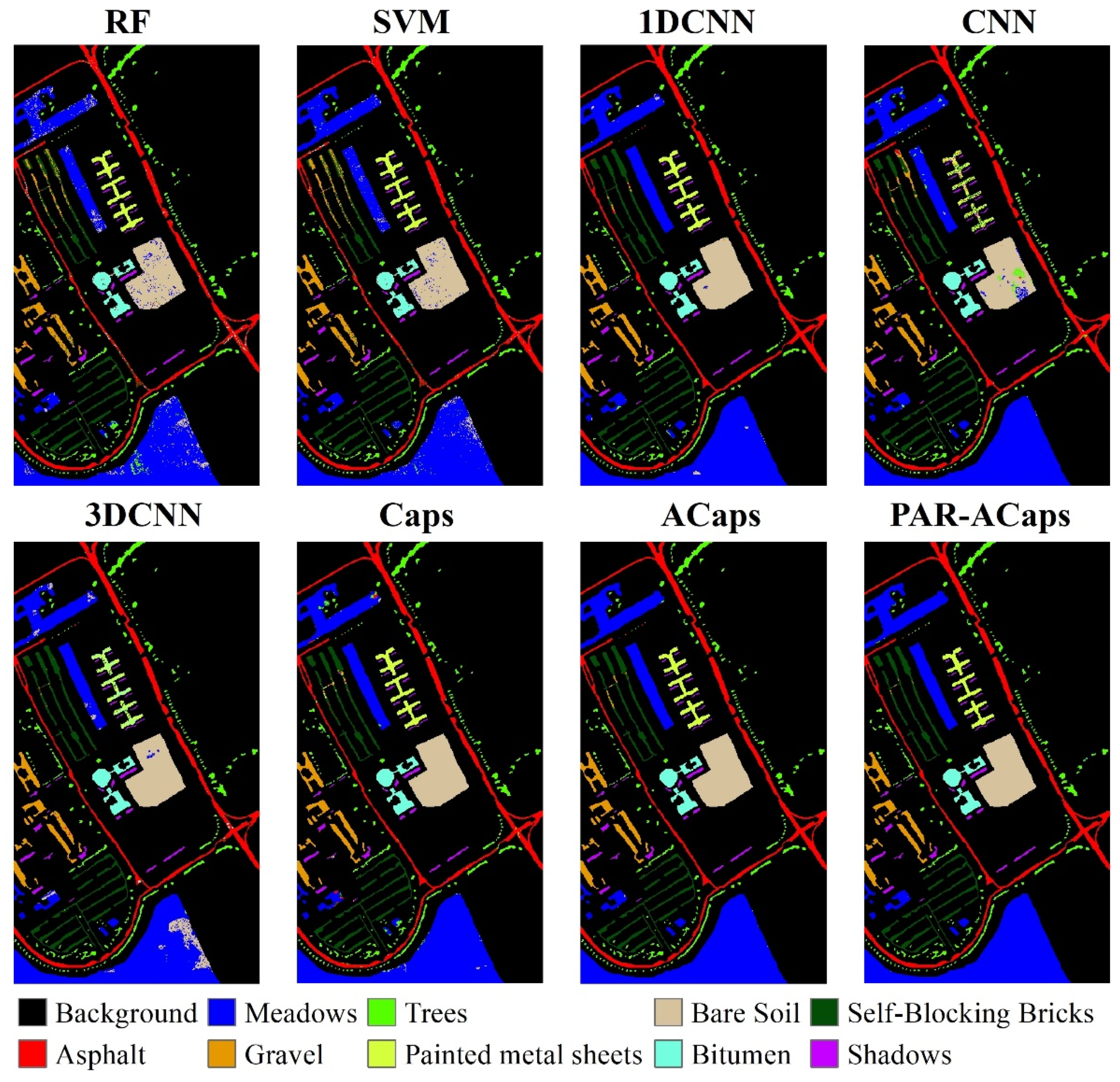
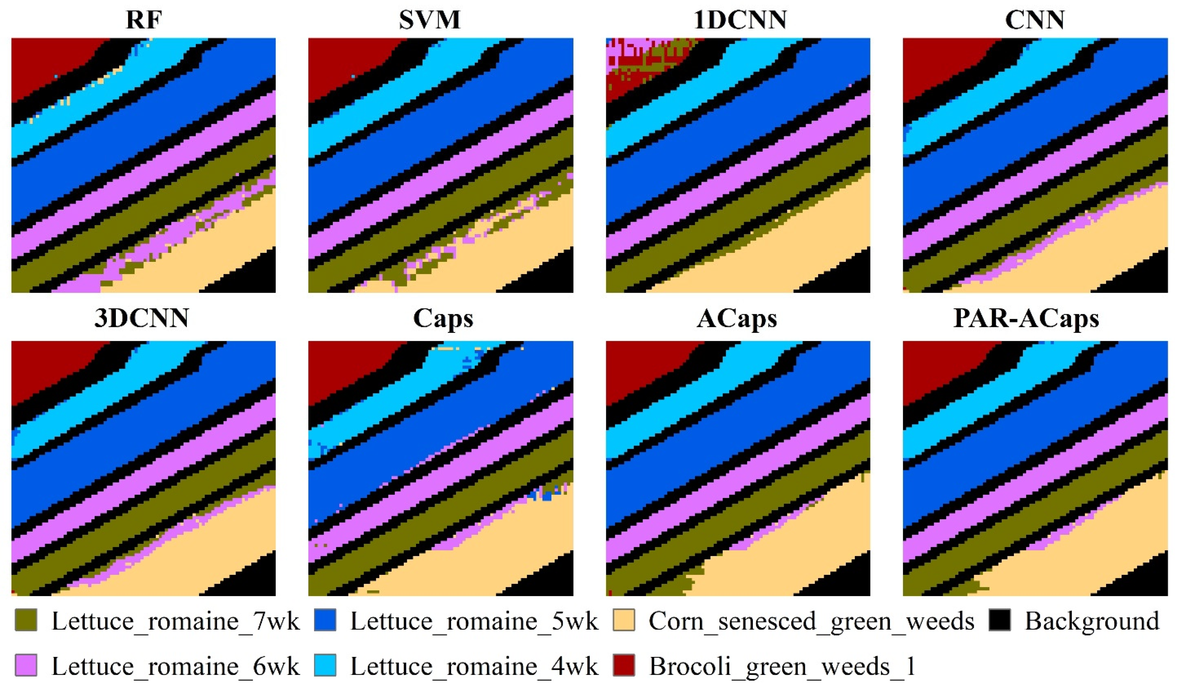
3.2.1. The Classification Performance of ACaps with Shallow Architecture

When the training processes were completed, the trained models were used to categorize the unlabeled test samples into the proper classes. The classification performances of the trained models were tested on the PU and SA dataset. The classification results obtained by the RF, SVM, 1DCNN, CNN, 3DCNN, and Caps-based models are shown in Figure 8 and Figure 9. For the PU dataset, the overall classification accuracy (OA) of RF, SVM, 1DCNN, CNN, 3DCNN, Caps, ACaps, and PAR-ACaps was 87.56%, 91.59%, 98.59%, 92.98%, 90.97%, 97.46%, 99.36, and 99.51%, respectively. The classification performances of the deep learning models were superior to those of RF and SVM. Specifically, the PAR-ACaps methods obtained the highest OA. As illustrated in Figure 8, most of the misclassifications occurred at the heterogeneous area that consisted of complex landscape structures or materials. For instance, many testing samples of Self-Blocking Bricks were misclassified as Gravel and Meadows in the classification results of RF, SVM, and CNN. Meanwhile, many samples of Meadows were misclassified as Bare Soil by 1DCNN and 3DCNN. By contrast, the misclassifications of ACaps and PAR-ACaps were slighter, and only a few samples of Self-Blocking Bricks were incorrectly classified as Gravel.

To further investigate the effectiveness of the PAR-ACaps for the PU dataset, the per-classification accuracy is presented in

Table 3. The overall accuracy (%), per-class accuracy (%), and the Kappa coefficients (K) between the PAR-ACaps and other classification methods in terms of classification accuracy with PU dataset; class names are in Table 1.

Class No.	RF	SVM	1DCNN	CNN	3DCNN	Caps	ACaps	PAR-ACaps
1	88.41	92.67	99.69	98.18	97.60	94.66	100	100
2	88.23	94.19	98.62	96.38	88.42	90.56	99.79	99.82
3	73.29	84.66	99.79	98.05	91.41	68.39	99.79	99.79
4	96.85	98.66	96.45	98.03	98.55	97.04	97.33	97.45
5	99.29	99.76	99.52	44.70	0.00	100	100	100
6	90.36	93.60	99.17	89.96	98.21	100	100	99.98
7	88.34	92.19	100	99.02	98.29	98.10	100	100
8	69.31	60.37	94.71	94.39	97.74	98.45	94.32	96.39
9	100	100	99.64	96.42	99.64	95.71	98.57	98.03
OA	87.56	91.59	98.59	94.49	90.97	97.46	99.36	99.51
K	0.82	0.87	0.97	0.91	0.87	0.96	0.98	0.99

. As shown by the table, the PAR-ACaps outperforms the benchmarks in terms of land-use/cover discrimination, especially for the complex class. For example, the classification accuracies of Meadows and Self-Blocking Bricks derived from PAR-ACaps were higher than those of the benchmarks.

As shown in Figure 9, the OAs obtained by the RF, SVM, 1DCNN, CNN, 3DCNN, Caps, ACaps, and PAR-ACaps for SA dataset were 73.43%, 81.56%, 83.65%, 93.92%, 85.05%, 86.66%, 92.75%, and 94.52%, respectively. The OAs of the benchmarks (i.e., RF, SVM, 1DCNN, CNN, 3DCNN, Caps, and ACaps) were lower than that of PAR-ACaps. Especially for the RF, SVM, 3DCNN, and Caps, many samples of Corn_senesced_green_weeds were misclassified as Lettuce_romaine_6wk and Lettuce_romaine_7wk. Specifically, the classification accuracies obtained by RF, SVM, 3DCNN, and Caps were only 2.93%, 29.66%, 45.64%, and 69.99%, respectively, as shown in

Table 4. The overall accuracy (%), per-class accuracy (%), and the Kappa coefficients (K) between the ACaps and other classification methods in terms of classification accuracy with SA dataset; class names are in Table 1.

Class No.	RF	SVM	1DCNN	CNN	3DCNN	Caps	ACaps	PAR-ACaps
1	99.47	99.47	51.15	100	100	100	100	99.86
2	2.93	29.66	87.78	92.06	45.64	69.99	72.29	82.46
3	87.97	96.83	99.18	96.30	93.35	79.90	99.36	98.18
4	100	100	99.93	99.71	100	93.93	100	98.41
5	100	100	100	99.47	100	97.24	100	99.70
6	99.66	100	100	100	98.99	93.47	99.33	97.99
OA	73.43	81.56	83.65	93.92	85.05	86.66	92.75	94.52
K	0.68	0.77	0.69	0.89	0.81	0.83	0.91	0.93

. In addition, many samples of Lettuce_romaine_4wk were misclassified as Lettuce_romaine_5wk by Caps, and the classification accuracy was only 79.90%, which is significantly lower than other classifiers. This led to the OAs of RF, SVM, 3DCNN, and Caps being far lower than those of CNN and PAR-ACaps. In contrast to the benchmarks, the OA of SA dataset was significantly improved by PAR-ACaps. Particularly, the classification accuracy of Corn_senesced_green_weeds was significantly improved and only lower than those of 1DCNN and CNN. Thus, the OA achieved by PAR-ACaps was the highest, and its outperformance can be clearly seen from Figure 9.

To check whether the improvement in classification performance of the PAR-ACaps had statistically significance, the McNemar’s test was used to analyze the classification method for a significance level of 0.05. The McNemar’s test was performed between the PAR-ACaps and the benchmarks. The p-values were calculated and are shown in

Table 5. The McNemar’s test results (p-value) derived from the quantitative comparisons of accuracy between the PAR-ACaps and the benchmarks (RF, SVM, 1DCNN, CNN, 3DCNN, Caps, and ACaps).

	Dataset	RF	SVM	1DCNN	CNN	3DCNN	Caps	ACaps
p-value	PU	0.0	0.0	2.674 × 10−12	3.458 × 10−15	4.327 × 10−19	1.806 × 10−16	1.046 × 10−9
	SA	3.863 × 10−134	7.238 × 10−64	9.652 × 10−32	8.773 × 10−43	6.984 × 10−33	6.698 × 10−38	3.675 × 10−12

. As shown in Table 5, the p-values were much smaller than 0.05. Thus, the improvement of the PAR-ACaps in classification performance appears to be important.

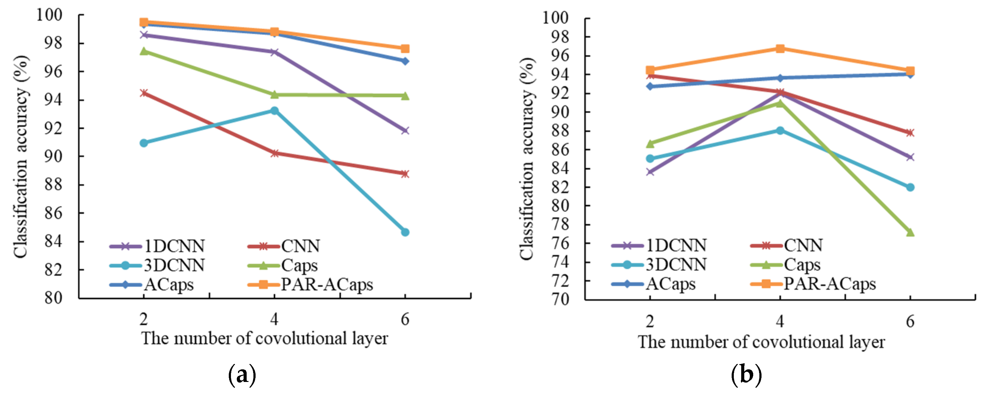
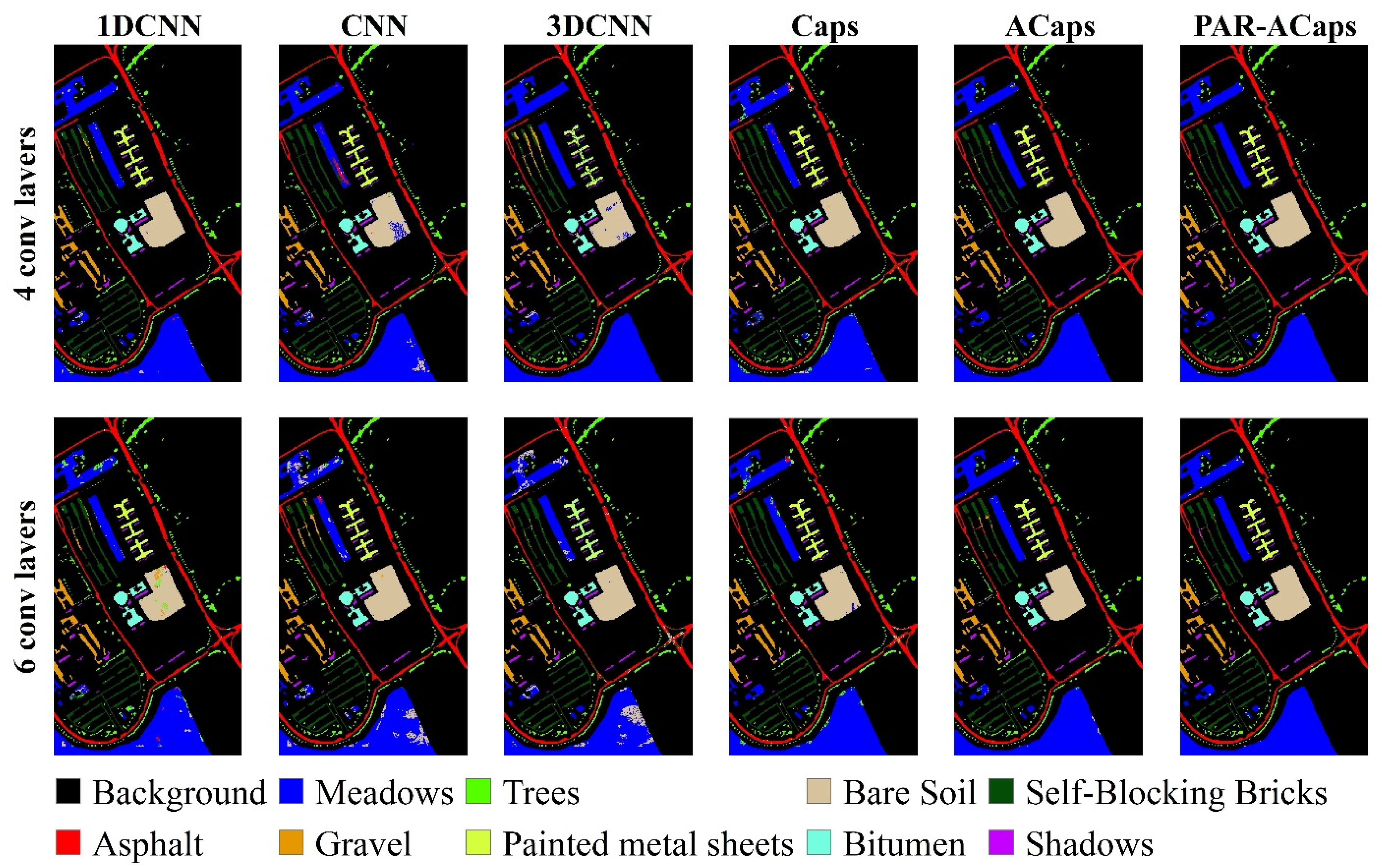
3.2.2. The Classification Performance of PAR-ACaps with Deeper Architecture

As mentioned above, the proposed model can avoid the gradient vanishing by removing the coupling coefficient $c_{ij}$ from the routing process and then introducing a hyperparameter $\gamma$ to amplify the gradient. To validate the effectiveness of the modification, the depths of the model architectures of 1DCNN, CNN, 3DCNN, Caps, ACaps, and PAR-ACaps were added, and then the classification performance of these models were tested on the PU and SA datasets. In this experiment, the number of feature extraction layers (convolutional layers) in 1DCNN, CNN, 3DCNN, Caps, ACaps, and PAR-ACaps were set as 4 and 6.

As illustrated in Figure 10a, the classification performances of 1DCNN, CNN, 3DCNN, and Caps for PU dataset significantly degenerated with the increase in the number of convolutional layers. The OAs of 1DCNN, CNN, 3DCNN, Caps, and ACaps decreased from 98.59%, 94.49%, 90.97%, 97.46%, and 99.36% to 91.84%, 88.79%, 84.67%, 94.31%, and 96.76%, respectively, with a decrease of 6.75%, 5.7%, 6.3%, 3.15%, and 2.60%. Compared with these benchmarks, the decrement of OA of PAR-ACaps was slighter with a decrease from 99.51% to 97.63%; the decline of PAR-ACaps was only 1.88%. The outperformance of PAR-ACaps with deeper architecture was also tested and verified on SA dataset (Figure 10b). The OA of PAR-ACaps decreased by 0.10% from 94.52%. The OA decline of PAR-ACaps was smaller than those of benchmarks including 1DCNN, CNN, 3DCNN, and Caps, which decreased from 91.98%, 93.92%, 85.05%, and 86.66% to 85.19%, 87.79%, 81.97%, and 77.18%, respectively.

In order to compare the classification performances of these models with deeper architectures in detail, the class-level classification results for PU and SA datasets are shown in

Table 6. The overall accuracy (%), per-class accuracy (%), and the Kappa coefficients (K) of PU dataset derived from CNN, Caps, ACaps, and PAR-ACaps with relatively deeper architectures.

4 convolutional layers
Class no.	1DCNN	CNN	3DCNN	Caps	ACaps	PAR-ACaps
1	98.55	94.83	94.70	88.68	99.27	99.20
2	97.06	87.82	99.05	95.74	98.70	98.75
3	98.15	96.06	98.77	96.72	99.79	99.69
4	97.67	91.71	97.56	91.05	96.89	97.11
5	100	97.94	0.00	99.05	100	100
6	99.65	91.31	93.81	99.58	99.93	99.94
7	100	96.09	88.04	98.45	98.78	99.26
8	90.91	88.25	67.84	87.95	96.13	97.29
9	97.50	95.80	100	87.61	95.00	96.07
OA	97.38	90.25	93.27	94.38	98.70	98.83
K	0.96	0.86	0.90	0.91	0.98	0.98
6 convolutional layers
1	97.99	98.91	81.42	93.09	95.65	97.32
2	90.38	85.99	81.32	93.71	98.01	98.34
3	97.54	98.97	91.20	97.34	97.34	97.95
4	97.11	96.89	98.11	90.63	94.12	95.28
5	98.82	96.75	0.00	98.47	98.35	98.47
6	87.52	99.73	99.86	97.90	99.96	99.82
7	98.78	98.82	99.02	99.02	99.26	99.63
8	87.43	77.19	95.29	94.90	85.37	90.07
9	94.64	96.35	99.64	87.67	90.71	93.92
OA	91.84	88.79	84.67	94.31	96.76	97.63
K	0.88	0.84	0.78	0.91	0.95	0.96

and

Table 7. The overall accuracy (%), per-class accuracy (%), and the Kappa coefficients (K) of SA dataset derived from CNN, Caps, ACaps, and PAR-ACaps with relatively deeper architectures.

4 convolutional layers
Class No.	1DCNN	CNN	3DCNN	Caps	Acaps	PAR-ACaps
1	100	100	100	100	100	100
2	71.40	68.24	58.61	68.56	75.84	89.43
3	95.56	97.40	90.50	96.04	98.73	98.10
4	100	98.94	100	99.91	100	99.82
5	100	99.84	100	100	100	100
6	99.33	98.32	100	96.99	100	98.66
OA	91.98	92.15	88.08	90.98	93.65	96.80
K	0.90	0.90	0.85	0.88	0.92	0.96
6 convolutional layers
1	100	99.47	100	97.73	100	100
2	47.42	57.66	39.07	44.87	77.50	79.18
3	91.13	92.19	84.17	65.50	98.52	98.10
4	100	99.43	100	97.72	99.94	100
5	100	99.86	100	85.43	100	100
6	98.99	99.44	98.32	90.07	100	100
OA	85.19	87.79	81.97	77.18	94.03	94.42
K	0.81	0.85	0.78	0.72	0.92	0.93

. From Table 6 and Table 7, the superiority of PAR-ACaps can be clearly observed, especially when distinguishing the most-often confused land cover/use types.

When performed on the PU dataset, the average OAs derived from 1DCNN, CNN, 3DCNN, Caps, ACaps, and PAR-ACaps with four convolutional layers were 97.38%, 90.25%, 93.27%, 94.38%, 98.70%, and 98.83%, respectively. Meanwhile, the OAs of these methods with six convolutional layers were 91.84%, 88.79%, 84.67%, 94.31%, 96.76%, and 97.63%, respectively. As illustrated in Figure 11, the misclassification phenomenon of 1DCNN, CNN, 3DCNN, and Caps were more serious than those of ACaps and PAR-ACaps, whereas the classification results of ACaps and PAR-ACaps with four and six convolutional layers were approximate to that of ACaps and PAR-ACaps with relatively shallower architecture, respectively.

As shown in Table 7 and Figure 12, the classification results of SA dataset also indicated that the performances of 1DCNN, CNN, 3DCNN, and Caps significantly degenerated with the increase in architecture depth. The average OAs derived from 1DCNN, CNN, 3DCNN, Caps, ACaps, and PAR-ACaps were 91.98%, 92.15%, 88.08%, 90.98%, 93.65%, and 96.80%, respectively, whereas the corresponding OAs decreased to 85.19%, 87.79%, 81.97%, 77.18%, 94.03%, and 94.42%, respectively. The numbers of samples that were misclassified by 1DCNN, CNN, 3DCNN, and Caps increased at a different degree. For example, the numbers of samples of Corn_Senesced_green_weeds, misclassified as Lettuce_romaine_6wk or Lettuce_romaine_6wk, increased with the depths of these networks.

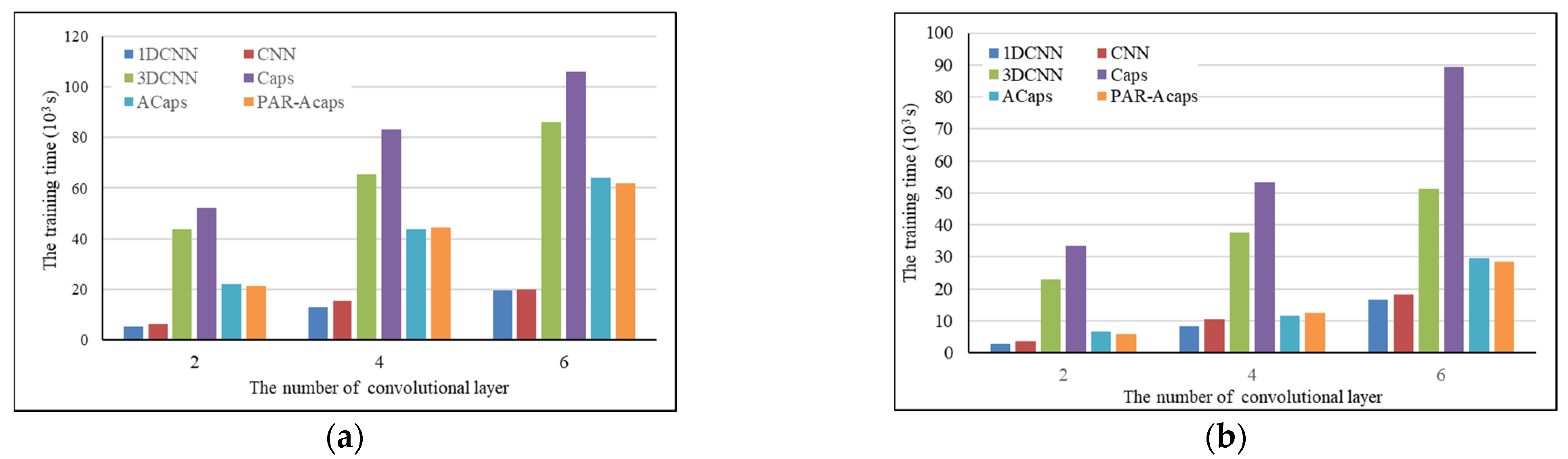
3.3. Computational Efficiency

For a fair comparison of computational efficiencies among the deep learning-based classifiers, the input window size of the CNN, 3DCNN, Caps, ACaps and PAR-ACaps were set as 31 × 31. The training time of these methods with two, four, and six convolutional layers for both PU and SA datasets are shown in Figure 13. The training time of these models increased with the number of convolutional layers. The training time of 1DCNN and Caps were, respectively, the least and the most for both PU and SA datasets. Meanwhile, it can be clearly seen that the training time of the Caps-based classifier was significantly reduced by the proposed method (PAR-ACaps) for both PU and SA datasets. The training time spent by the Caps with a different number of convolutional layers for PU and SA dataset was about 2 times of those of the ACaps and PAR-ACaps with similar network structures.

4. Discussion

This paper proposed a kind of powered activation regularization (PAR)-based adaptive capsule network (PAR-ACaps) that uses adaptive routing algorithm without iteration for the purpose of feature relationship learning and PAR method for more discriminative feature learning. The classification performance of PAR-ACaps was tested on two public datasets (i.e., PU and SA dataset) and compared with that of the benchmarks including RF, SVM, 1DCNN, CNN, 3DCNN, Caps, and ACaps. To further verify the effectiveness of the routing algorithm without iteration, the classification performance of PAR-ACaps with relatively deeper architecture was also compared with those of 1DCNN, CNN, 3DCNN, Caps, and ACaps with the same number of convolutional layers. The experimental results verified that the classification performances of PAR-ACaps with shallow and relatively deeper architecture were superior to those of the benchmarks in terms of OA, and the computational efficiency of the PAR-ACaps was significantly improved from the original Caps.

Unlike the CNN that uses the pooling layer to reduce the dimension of the features and avoid the phenomenon of overfit, PAR-ACaps uses the routing algorithm to replicate the learned knowledge across the space. Thus, the spatial information (e.g., the precise position of entity) would not be thrown away and the relationship among the features can be learned. Therefore, the classification performance of PAR-ACaps in terms of OA is superior to those of 1DCNN, CNN, and 3DCNN. Due to the phenomenon of coupling coefficient thinning gradually in the training process of Caps, the gradient vanishes and thus may lead to suboptimal probability distribution. Meanwhile, the PAR-ACaps introduced the hyperparameter $\gamma$ into the routing process to amplify the gradient, and the adaptive routing algorithm was thus proposed for solving the problem of gradient vanishing in Caps. Furthermore, the PAR method was proposed and used to repress the strength of connections of capsules in adjacent capsule layers, and the sparser, and more discriminative representation was thus learned to improve the classification performance. The outperformances of PAR-ACaps with relatively shallower and deeper architectures demonstrated that the adaptive routing algorithm and PAR method are effective to the problem faced by the Caps and ACaps, respectively. Simultaneously, there is no iteration process in the adaptive routing algorithm, and the computational efficiency of PAR-ACaps was significantly higher than that of Caps. However, the number of trainable parameters of the Caps- and ACaps-based classification methods were larger than that of CNN-based methods, and the training time consumed by Caps and ACaps-based classification methods were thus far more than those of CNN-based methods.

5. Conclusions

In this study, a new hyperspectral remote sensing classification method based on an improved adaptive capsule network (PAR-ACaps) was proposed in which gradient vanishing and overfitting were avoided by using an adaptive routing algorithm. The PAR method was proposed and used to learn sparser and more discriminative representation. The performance of the proposed PAR-ACaps was tested with two public datasets (PU and SA dataset) by measuring the OAs and the training time. The experimental results demonstrated that the proposed method with shallow and relatively deeper architecture could always achieve the highest classification accuracies, constantly outperforming benchmark comparisons including RF, SVM, 1DCNN, CNN, 3DCNN, Caps, and ACaps. In terms of the computational efficiency, the proposed method has significantly reduced the time consumed by Caps-based method. We, therefore, conclude that the proposed PAR-ACaps has great potential for the hyperspectral remote sensing classification. However, the pixel-wise method (PAR-ACaps) cannot reduce the salt-and-pepper noise [32]. To further improve the classification performance of the Caps-based classifier, object-oriented Caps-based classifier is needed. In the future, we will further study the object-oriented capsule network.

References

1. Feddema, J.J.; Oleson, K.W.; Bonan, G.B.; Mearns, L.O.; Buja, L.E.; Meehl, G.A.; Washington, W.M. The importance of land-cover change in simulating future climates. Science 2005, 310, 1674–1678. [Google Scholar] [CrossRef] [Green Version]
2. Ding, X.; Zhang, S.; Li, H.; Wu, P.; Dale, P.; Liu, L.; Cheng, S. A restrictive polymorphic ant colony algorithm for the optimal band selection of hyperspectral remote sensing images. Int. J. Remote Sens. 2020, 41, 1093–1117. [Google Scholar] [CrossRef]
3. Hu, Y.; Zhang, J.; Ma, Y.; An, J.; Ren, G.; Li, X. Hyperspectral coastal wetland classification based on a multiobject convolutional neural network model and decision fusion. IEEE Geosci. Remote Sens. Lett. 2019, 16, 1110–1114. [Google Scholar] [CrossRef]
4. Ding, X.; Li, H.; Yang, J.; Dale, P.; Chen, X.; Jiang, C.; Zhang, S. An improved ant colony algorithm for optimized band selection of hyperspectral remotely sensed imagery. IEEE Access 2020, 8, 25789–25799. [Google Scholar] [CrossRef]
5. Hinton, G.E.; Salakhutdinov, R.R. Reducing the dimensionality of data with neural networks. Science 2006, 313, 504–507. [Google Scholar] [CrossRef] [PubMed] [Green Version]
6. Bera, S.; Shrivastava, V.K. Analysis of various optimizers on deep convolutional neural network model in the application of hyperspectral remote sensing image classification. Int. J. Remote Sens. 2020, 41, 2664–2683. [Google Scholar] [CrossRef]
7. Liang, M.; Hu, X. Recurrent convolutional neural network for object recognition. In Proceedings of the IEEE Conference on Computer Vision and Pattern Recognition, Boston, MA, USA, 7–12 June 2015; pp. 3367–3375. [Google Scholar]
8. Li, H.; Zhang, C.; Zhang, S.; Atkinson, P.M. A hybrid OSVM-OCNN method for crop classification from fine spatial resolution remotely sensed imagery. Remote Sens. 2019, 11, 2370. [Google Scholar] [CrossRef] [Green Version]
9. Zhang, C.; Pan, X.; Li, H.; Gardiner, A.; Sargent, I.; Hare, J.; Atkinson, P.M. A hybrid MLP-CNN classifier for very fine resolution remotely sensed image classification. ISPRS J. Photogramm. Remote Sens. 2018, 140, 133–144. [Google Scholar] [CrossRef] [Green Version]
10. Othman, E.; Bazi, Y.; Alajlan, N.; Alhichri, H.; Melgani, F. Using convolutional features and a sparse autoencoder for land-use scene classification. Int. J. Remote Sens. 2016, 37, 2149–2167. [Google Scholar] [CrossRef]
11. Sharma, A.; Liu, X.; Yang, X.; Shi, D. A patch-based convolutional neural network for remote sensing image classification. Neural Netw. 2017, 95, 19–28. [Google Scholar] [CrossRef] [PubMed]
12. Chen, Y.; Jiang, H.; Li, C.; Jia, X.; Ghamisi, P. Deep Feature Extraction and Classification of Hyperspectral Images Based on Convolutional Neural Networks. IEEE Trans. Geosci. Remote. Sens. 2016, 54, 6232–6251. [Google Scholar] [CrossRef] [Green Version]
13. Alam, F.I.; Zhou, J.; Liew, A.W.C.; Jia, X. CRF learning with CNN features for hyperspectral image segmentation. In Proceedings of the 2016 IEEE International Geoscience and Remote Sensing Symposium (IGARSS), Beijing, China, 10–15 July 2016; IEEE: New York, NY, USA, 2016; pp. 6890–6893. [Google Scholar]
14. Gong, Z.; Zhong, P.; Yu, Y.; Hu, W.; Li, S. A CNN with multiscale convolution and diversified metric for hyperspectral image classification. IEEE Trans. Geosci. Remote Sens. 2019, 57, 3599–3618. [Google Scholar] [CrossRef]
15. Khotimah, W.N.; Bennamoun, M.; Boussaid, F.; Sohel, F.; Edwards, D. A High-Performance Spectral-Spatial Residual Network for Hyperspectral Image Classification with Small Training Data. Remote Sens. 2020, 12, 3137. [Google Scholar] [CrossRef]
16. Xiang, C.; Zhang, L.; Tang, Y.; Zou, W.; Xu, C. ACaps: A novel multi-scale capsule network. IEEE Signal Process. Lett. 2018, 25, 1850–1854. [Google Scholar] [CrossRef]
17. Sabour, S.; Frosst, N.; Hinton, G.E. Dynamic routing between capsules. In Advances in Neural Information Processing Systems; MIT Press: Cambridge, MA, USA, 2017; pp. 3856–3866. [Google Scholar]
18. Ren, Q.; Shang, S.; He, L. 2019 Adaptive Routing Between Capsules. arXiv 2019, arXiv:1911.08119. [Google Scholar]
19. Nguyen, C.D.T.; Dao, H.H.; Huynh, M.T.; Phu Ward, T. ResCap: Residual Capsules Network for Medical Image Segmentation. In Proceedings of the 2019 Kidney Tumor Segmentation Challenge: KiTS19, Shenzhen, China, 13 October 2019. [Google Scholar]
20. Chen, R.; Jalal, M.A.; Mihaylova, L. Learning capsules for vehicle logo recognition. In Proceedings of the 2018 21st International Conference on Information Fusion, Cambridge, UK, 10–13 July 2018; pp. 565–572. [Google Scholar]
21. Duarte, K.; Rawat, Y.; Shah, M. Videocapsulenet: A simplified network for action detection. In Advances in Neural Information Processing Systems; 2018; pp. 7610–7619. Available online: https://dl.acm.org/doi/10.5555/3327757.3327860 (accessed on 18 May 2021).
22. Beşer, F.; Kizrak, M.A.; Bolat, B.; Yildirim, T. Recognition of sign language using capsule networks. In Proceedings of the 2018 26th Signal Processing and Communications Applications Conference (SIU), Izmir, Turkey, 2–5 May 2018; pp. 1–4. [Google Scholar]
23. Paoletti, M.E.; Haut, J.M.; Fernandez-Beltran, R.; Plaza, J.; Plaza, A.; Li, J.; Pla, F. Capsule networks for hyperspectral image classification. IEEE Trans. Geosci. Remote Sens. 2018, 57, 2145–2160. [Google Scholar] [CrossRef]
24. Wang, W.Y.; Li, H.C.; Pan, L.; Yang, G.; Du, Q. Hyperspectral Image Classification Based on Capsule Network. In Proceedings of the IGARSS 2018-2018 IEEE International Geoscience and Remote Sensing Symposium, Valencia, Spain, 22–27 July 2018; pp. 3571–3574. [Google Scholar]
25. Deng, F.; Pu, S.; Chen, X.; Shi, Y.; Yuan, T.; Pu, S. Hyperspectral image classification with capsule network using limited training samples. Sensors 2018, 18, 3153. [Google Scholar] [CrossRef] [PubMed] [Green Version]
26. Zhao, Z.; Kleinhans, A.; Sandhu, G.; Patel, I.; Unnikrishnan, K.P. Capsule networks with max-min normalization. arXiv 2019, arXiv:1903.09662. [Google Scholar]
27. Jia, B.; Huang, Q. DE-CapsNet: A diverse enhanced capsule network with disperse dynamic routing. Appl. Sci. 2020, 10, 884. [Google Scholar] [CrossRef] [Green Version]
28. Kwabena, P.M.; Weyori, B.A.; Mighty, A.A. Exploring the performance of LBP-capsule networks with K-Means routing on complex images. J. King Saud Univ. Comput. Inf. Sci. 2020. [Google Scholar] [CrossRef]
29. Yang, Z.; Wang, X. Reducing the dilution: An analysis of the information sensitiveness of capsule network with a practical solution. arXiv 2019, arXiv:1903.10588. [Google Scholar]
30. Hinton, G.E.; Sabour, S.; Frosst, N. Matrix capsules with EM routing. In Proceedings of the International Conference on Learning Representations, Vancouver, BC, Canada, 30 April–3 May 2018. [Google Scholar]
31. De Leeuw, J.; Jia, H.; Yang, L.; Liu, X.; Schmidt, K.; Skidmore, A.K. Comparing accuracy assessments to infer superiority of image classification methods. Int. J. Remote Sens. 2006, 27, 223–232. [Google Scholar] [CrossRef]
32. Zhang, C.; Sargent, I.; Pan, X.; Li, H.; Gardiner, A.; Hare, J.; Atkinson, P.M. An object-based convolutional neural network (OCNN) for urban land use classification. Remote Sens. Environ. 2018, 216, 57–70. [Google Scholar] [CrossRef] [Green Version]
Figure 1. Capsule network with three layers for the classification of MNIST dataset [11].
Remotesensing 13 02445 g001
Figure 2. (a) The SA dataset; and (b) ground truth for the same area of the Salinas Valley.
Remotesensing 13 02445 g002
Figure 3. (a) The PU dataset; and (b) ground truth for the same area of Pavia University.
Remotesensing 13 02445 g003
Figure 4. The computational process of the capsules.
Remotesensing 13 02445 g004
Figure 5. The architecture of PAR-ACaps and the adaptive routing process. Encoding part consists of feature extraction and capsule encoding stages. Decoder part includes DigitCaps layer and dense layers which reconstruct an image from DigitCaps layer representation. FC denotes the fully connected layer. d 0 is the dimension of the digital capsule. N c is the number of classes. d 1 denotes the dimension of the output of dense layers. Sigmoid represent the activation functions of sigmoid function in FC layer.
Remotesensing 13 02445 g005
Figure 6. The network architectures of 1DCNN, CNN, 3DCNN, Caps, Acaps, and PAR-ACaps. The red lines with an arrow represent the data flows in the CNN-based models. In comparison, the blue lines denote the data flows in the Caps-based models.
Remotesensing 13 02445 g006
Figure 7. The influence of the input window size on the overall classification accuracy of CNN and Caps method for both SA and PU datasets. (a) The influence of the input window size of CNN, and (b) the influence of the input window size of Caps.
Remotesensing 13 02445 g007
Figure 8. The classification results of PU dataset obtained by the PAR-ACaps and the benchmarks.
Remotesensing 13 02445 g008
Figure 9. The classification results of SA dataset obtained by the PAR-ACaps and the benchmarks.
Remotesensing 13 02445 g009
Figure 10. The changes of the classification accuracies of the 1DCNN, CNN, 3DCNN, Caps, ACaps, and PAR-ACaps for PU and SA datasets. (a) Classification accuracies derived from PU dataset. (b) Classification accuracies derived from SA dataset.
Remotesensing 13 02445 g010
Figure 11. The classification results of PU dataset derived from 1DCNN, CNN, 3DCNN, Caps, ACaps, and PAR-ACaps with four and six convolutional layers.
Remotesensing 13 02445 g011
Figure 12. The classification results of SA dataset derived from 1DCNN, CNN, 3DCNN, Caps, ACaps, and PAR-ACaps with four and six convolutional layers.
Remotesensing 13 02445 g012
Figure 13. The training time of 1DCNN, CNN, 3DCNN, Caps, ACaps, and PAR-ACaps with a different number of convolutional layers (two, four, and six). (a) The training time for PU dataset and (b) the training time for SA dataset.
Remotesensing 13 02445 g013