Article

Identification of Significative LiDAR Metrics and Comparison of Machine Learning Approaches for Estimating Stand and Diversity Variables in Heterogeneous Brazilian Atlantic Forest

by
Rorai Pereira Martins-Neto
1,*,
Antonio Maria Garcia Tommaselli
1,2,
Nilton Nobuhiro Imai
1,2,
Hassan Camil David
3,
Milto Miltiadou
4,5 and
Eija Honkavaara
6
1
Graduate Program in Cartographic Sciences, São Paulo State University (UNESP), Roberto Simonsen 305, Presidente Prudente 19060-900, SP, Brazil
2
Department of Cartography, São Paulo State University (UNESP), Roberto Simonsen 305, Presidente Prudente 19060-900, SP, Brazil
3
Department of Forestry, Federal Rural University of Amazonia (UFRA), Tv. Pau Amarelo s/n, Capitão Poço 68650-000, PA, Brazil
4
ERATOSTHENES Centre of Excellence, Limassol 3036, Cyprus
5
Laboratory of Remote Sensing and Geo-Environment, Department of Civil Engineering and Geomatics, School of Engineering and Technology, Cyprus University of Technology, Limassol 3036, Cyprus
6
Finnish Geospatial Research Institute (FGI), National Land Survey of Finland, Geodeetinrinne 2, 02430 Masala, Finland
*
Author to whom correspondence should be addressed.
Remote Sens. 2021, 13(13), 2444; https://doi.org/10.3390/rs13132444
Submission received: 24 May 2021 / Revised: 16 June 2021 / Accepted: 17 June 2021 / Published: 23 June 2021
(This article belongs to the Special Issue Remote Sensing for Agricultural, Environmental and Forestry Policies)

Abstract

:
Data collection and estimation of variables that describe the structure of tropical forests, diversity, and richness of tree species are challenging tasks. Light detection and ranging (LiDAR) is a powerful technique due to its ability to penetrate small openings and cracks in the forest canopy, enabling the collection of structural information in complex forests. Our objective was to identify the most significant LiDAR metrics and machine learning techniques to estimate the stand and diversity variables in a disturbed heterogeneous tropical forest. Data were collected in a remnant of the Brazilian Atlantic Forest with different successional stages. LiDAR metrics were used in three types of transformation: (i) raw data (untransformed), (ii) correlation analysis, and (iii) principal component analysis (PCA). These transformations were tested with four machine learning techniques: (i) artificial neural network (ANN), ordinary least squares (OLS), random forests (RF), and support vector machine (SVM) with different configurations resulting in 27 combinations. The best technique was determined based on the lowest RMSE (%) and corrected Akaike information criterion (AICc), and bias (%) values close to zero. The output forest variables were mean diameter at breast height (MDBH), quadratic mean diameter (QMD), basal area (BA), density (DEN), number of tree species (NTS), as well as Shannon–Waver (H’) and Simpson’s diversity indices (D). The best input data were the new variables obtained from the PCA, and the best modeling method was ANN with two hidden layers for the variables MDBH, QMD, BA, and DEN while for NTS, H’and D, the ANN with three hidden layers were the best methods. For MDBH, QMD, H’and D, the RMSE was 5.2–10% with a bias between −1.7% and 3.6%. The BA, DEN, and NTS were the most difficult variables to estimate, due to their complexity in tropical forests; the RMSE was 16.2–27.6% and the bias between −12.4% and −0.24%. The results showed that it is possible to estimate the stand and diversity variables in heterogeneous forests with LiDAR data.

Graphical Abstract

1. Introduction

Field surveys in the Brazilian tropical forests (e.g., Atlantic forest) are laborious work. The high understory density, presence of lianas and vines, and aerial roots existent in this environment result in difficulties for the measurement of tree variables and a walk through the forest. Estimating variables that describe the forest structure, the tree species diversity, and richness are challenging tasks, because the Brazilian Atlantic forest is a very rich biome in plant species, with approximately 14,000 vascular plant species, of which approximately 8000 are classified as endemic [1]. Additionally, measuring the canopy area and tree heights is troublesome because of the variation in tree height and overlapping of tree crowns. Due to these restrictions, tree height is usually estimated with the naked eye [2]. These data are often used as inputs for regression models to estimate biomass, volume, growth, and yield, but uncertainties in the field variables measurement propagate to the estimates through regression models [3,4].
Data from airborne laser scanner (ALS) have been widely used in forestry applications, due to their ability to penetrate through small openings (e.g., gaps between branches and leaves) in the forest canopy and collect three-dimensional information of vegetation and terrain [5,6,7]. ALS is based on light detection and ranging (LiDAR) technology, and with the resulting three-dimensional point cloud, it is possible to better understand the arrangement of the forest canopy, allowing the accurate estimation of structural parameters of the forest [8]. The information acquired by ALS is very valuable for forest inventory and modeling, especially for dense, complex forests that are not safe and/or easy to access.
It is possible to extract several metrics from the ALS point cloud. This includes descriptive statistics, percentiles, and distribution measures of heights, intensity, and laser pulse returns, providing a summary of the forest canopy structure. LiDAR metrics are usually used as predictors in regression models for the estimation of forest biophysical variables [9,10,11]. Multiple linear regression is commonly used for modeling forest variables from LiDAR metrics due to its simplicity and clarity when interpreting the resulting model [12].
However, multiple linear regression requires the basic assumptions of classical statistics, which can be difficult to achieve when dealing with the modeling of biological data [13]. As a result, the use of computational techniques, such as machine learning, has been increased, including modeling forest inventory variables with LiDAR metrics as predictors. Machine learning techniques can model complex relationships between dependent and independent variables (i.e., a large number of LiDAR metrics) without requiring linear assumptions about the data distribution [13,14]. Therefore, machine learning techniques are suitable for predicting complex non-linear relationships. Additionally, interaction effects are modeled automatically which makes these methods very powerful and promising compared to multiple linear regression to estimate forest parameters from LiDAR data [13,15].
The use of LiDAR metrics to estimate forest variables using machine learning techniques has been used in forest plantations in Brazil. The estimate of total, commercial, and pulp volume of a Pinus taeda plantation was performed by Silva et al. [16] using LiDAR metrics as input data for the random forest (RF) algorithm. The results obtained indicated a low bias prediction (average of −0.2%) and the average of the root-mean-square error (RMSE) was 8.1%. The authors concluded the use of RF to determine different types of volumes in homogeneous forests presents highly accurate estimates. In Eucalyptus spp. plantations, Görgens et al. [17] estimated volume per stand comparing multiple linear regression with artificial neural network (ANN), RF, and support vector machine (SVM) regression methods. The results obtained reached high accuracy, with R² close to 0.90 and with bias tending to zero. Among the tested machine learning methods, RF was slightly better than the other methods and its results were similar to the results obtained with multiple linear regression. The assessment of ANN, k nearest neighbors, and RF for modeling trunk shape and volume in black wattle plantation, [18] showed that ANN and RF presented the best results, with RMSE of 8% and 8.4%, respectively, against the RMSE of 9.15% for the polynomial model. The authors concluded that the machine learning techniques are appropriate for forest modeling, however, their use should be cautious because of the greater possibility of overtraining and overfitting.
Regarding native Brazilian forests, the combination of LiDAR metrics and machine learning techniques is mainly focused on the Amazonian forest to estimate the aboveground biomass. In low-intensity logging areas, [19] estimated the aboveground biomass (AGB) stock by comparing multiple linear regression with some machine learning approaches. Linear regression was the most appropriate method for the case study, with an RMSE of 19.7%, slightly better than the methods of RF, ANN, and SVM with a RMSE of 22.8% for the three methods. However, the results demonstrate the potential for predicting AGB when a non-parametric method is required mainly in tropical forests, due to its great diversity and heterogeneity.
Nevertheless, there are other biomes in Brazil with high richness and species diversity such as the Atlantic Forest. This is the second-largest rainforest in America, which occurs mainly along the coast, extending far inland in some areas of south and southeastern Brazil [20], whose composition, structure, and diversity remain mostly unknown. Due to the occupation of the national territory that mainly occurs along the coast and other anthropogenic activities (e.g., logging, disordered urban growth, agricultural encroachment, and industrialization), the Atlantic Forest is the most degraded biome in Brazil. It is approximated that only 11.6% of its original cover still remains, and these are very fragmented [21,22,23]. However, this biome is a biodiversity hotspot because it has already lost more than 75% of its original cover, with very high fragmentation, the remaining forest fragments of this biome have a high species endemism [24,25].
The semideciduous seasonal forest, also known as inland Atlantic Forest because of the inland location, is one of the phytophysiognomies and associated ecosystems defining and forming the Atlantic forest, as described by [26]. Despite the importance of this native forest, it is often neglected, resulting in a lack of information about its composition, structure, and diversity [27].
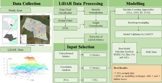
The lack of studies using LiDAR metrics in the Brazilian Atlantic Forest and their potential for estimating variables describing the forest structure was the motivation for this work. The main objective is to compare four machine learning approaches (ANN, ordinary least-squares multiple regression (OLS), RF, and SVM) with different numbers of LiDAR metrics as input data, to estimate seven stand and diversity variables: mean diameter at breast height (MDBH), quadratic mean diameter (QMD), basal area (BA), density (DEN), number of tree species (NTS), Shannon–Waver diversity index (H’), and Simpson diversity index (D). An area-based approach was considered more applicable than individual tree-based techniques due to the difficulty of extracting individual trees in the tropical forest [28,29].
An extensive experimental assessment was made, combining the three input types of LiDAR metrics with the different regression methods tested with different architectures, to estimate the stand and diversity forest variables cited. The results obtained in this study may contribute to finding the best combination of a selection of metrics to deal with and a machine learning technique to estimate forest variables in an inland Atlantic Forest.

2. Materials and Methods

2.1. Field Survey

The study was carried out in a remnant of inland Atlantic Forest, named Ponte Branca (White Bridge), located in the west of São Paulo State, Brazil. Its size is approximately 13 km² (Figure 1). As described by Berveglieri et al. [30], this forest remnant has suffered from disturbances over time like selective logging and forest fires. However, there are still areas at a good conservation state. Different successional stages are found from pioneer formations to advanced regeneration stages with late secondary and climax species in the upper canopy. The understory is dominated by the Myrtaceae family, mainly by the Eugenia uniflora species, and with a high occurrence of Dendropanax cuneatus. In the upper canopy the species Aspidosperma spp., Copaifera langsdorffii, and Hymenaea courbaril are found.
Field data were collected in seven square plots of 40 m × 40 m and eight rectangular plots with dimensions of 80 m × 20 m. This sums up to a total of 15 plots with an area of 1600 m² each (Figure 1). Plots 8 to Plot 15 have different dimensions due to greater observed heterogeneity in successional stages found in each plot. As a result, rectangular plots better represent the differences in these areas. The allocation of each plot was based on the previous interpretation of historical and recent aerial images and on the management plan provided by the environmental agency responsible for the study area, in such a way that the plots covered all successional stages present in the Ponte Branca forest remnant. In [30,31], a detailed description of the successional stages in the study area is presented. The sampling area was 0.2% of the total forested area. The four corner positions of each plot were obtained by a dual-frequency Global Navigation Satellite System receiver with, at least, one-hour tracking, achieving an estimated precision of approximately 50 cm. The area did not have continuous inventory data due to the restricted accessibility caused by the high density of trees, and vines within the forest remnant. Despite the accessibility limitations, it was possible to survey a sample of plots for this study.
All trees with DBH (Diameter at Breast Height) above 3.5 cm were counted, individually measured, and their tree species were identified. From the measured DBH the variables MDBH (cm), QMD (cm), and BA (m² ha−1) were calculated. From the tree counting, DEN (trees ha−1) was obtained, and from the cataloged species, the total number of tree species per plot (NTS) was calculated. The Shannon–Weaver diversity index, H’ (Equation (1)) [32], and the Simpson index D (Equation (2)) [33], were also calculated to understand species composition and diversity. A summary of the seven variables obtained in the field is shown in Table 1, and the statistics of the variables for each of the 15 surveyed plots are presented in the Supplementary Materials (Table S1).
H = i = 1 S p i ln p i
where H′ is the Shannon–Weaver diversity index, S is the total number of species sampled and p i is the ratio of the number of individual trees sampled from the ith species to the total number of individual trees.
D = 1 n i n i 1 N N 1
where D is the Simpson index, n is the number of individual trees of the i th species and N is the total number of individual trees.

2.2. LiDAR Data Collection

The LiDAR data covering the study area was acquired in October 2017. The airborne laser scanner used was a RIEGL LMS-Q680i, which is a full-waveform LiDAR sensor with a scan angle range of ±30°. The waveforms were processed in post-processing mode and the point cloud was the peak returns of the waveforms that were delivered in discrete LiDAR file formats. Up to 5 returns per emitted pulse were recorded, which is allowed according to the specifications of the .las file [34]. This scanner model uses the multiple time around (MTA) technique due to the high frequency of repetition (up to 400,000 Hz), being able to acquire echoes arriving after a delay of more than one pulse repetition interval, thus allowing measurements with a range beyond the maximum unambiguous measurement range [35].
The flight height of the LiDAR survey used in the study was 900 m. The LiDAR data was delivered in 16 flight lines acquired in the northeast-southwest direction, and covering the entire Ponte Branca forest remnant. The average sampling density was 19.8 pulses per m2. Figure 2 depicts the ALS point cloud of a plot of the study area, showing a sample of the vertical structure of the forest.

2.3. LiDAR Data Processing

For LiDAR data processing, LAStools [36] and R environment [37] have been utilized, to obtain area-based metrics from the point clouds. First, with LAStools [36], the classification of the point cloud into ground and nonground points was performed. Several parameters were empirically assessed to achieve suitable results, mainly ensuring that ground points always existed within the selected search window, since in tropical forests there is a dense understory, and ground points are sometimes not acquired by LiDAR systems.
The following processing steps were performed in the R environment [37] using the LidR package [38]. The main aim was to extract LiDAR metrics, not only related to elevation and pulse returns, but also to intensity metrics, to understand their relationship in estimating forest variables. However, the distance between the sensor and the target is not constant during the survey, due to the variations of the platform (aircraft), the terrain topography [39,40,41,42], and the scan angle. These variations in the distances and atmospheric attenuation change the intensity recorded by the sensor [40,43,44]. Even with these variations, some authors used raw intensities [45,46,47]. However, to achieve more accurate results, the use of intensity metrics requires a priori correction also known as normalization. In this study, we used a range correction model (Equation (3)) developed by [40,43], which is based on the distance traveled from the sensor beam to the target is not the same [42].
I n o r m = I o b s R a c t R r e f f
where I n o r m is the normalized intensity, I o b s is the observed intensity, R a c t is the distance between the laser instrument and the returns, R r e f is an arbitrary reference distance, f represents the rate of energy attenuation sustained by the pulse as it travels through a medium back and forth from a target.
To calculate the R a c t parameter for each return, it was necessary to determine the location of the sensor, which was performed using a method proposed by [42], which is an adaptation of the methodology developed by [43]. The main idea is that a pair of very close pulses on different flight lines, assuming they reach the same object, must have the same intensity. If there is a difference it would be indicative of a difference of range [42]. Thus, the sensor’s position was determined by linear interpolation from the two closest points in the aircraft’s trajectory positions, then the range for each return was determined as the Euclidean distance from the point to the sensor [42,43]. To apply this method, the values of ’gpstime’, ’ReturnNumber’, ’NumberOfReturns’, and ’PointSourceID’ are necessary [38], which are not always made available by the data provider, making normalization of intensity unviable [40,41,42,43]. Our data had all these values, so it was possible to proceed with the intensity normalization.
We use the arbitrary reference distance as the flight height, that is, 900 m. In forest areas, the optimum value of the exponent f should be between 2.1–2.5 [43], but for practical purposes, the values between 2.2 to 2.4 are the most suitable, according to [42]. We made some preliminary experiments and the value of 2.3 was the best choice for our area of study. After this procedure, the result was a point cloud with corrected (or normalized) intensity values, with which it was possible to extract intensity metrics and to use them as predictor variables. The Riegl LMS-Q680i instrument records pulses with an intensity of 16 bits, but processing and analyzing huge datasets with this range is costly and thus, the intensity data were resampled to 8 bits.
A point cloud with corrected intensities, containing only ground points was modeled using a triangular irregular network (TIN) to generate a digital terrain model (DTM), with a sample distance of 0.50 m. The point cloud (once ground points were removed) was normalized using the DTM. The result is a normalized point cloud with only vegetation-related points included, mapped on flat terrain. After that, outliers were removed according to the expected heights of the trees existing in the area; points below 0 m and above 40 m were removed. The normalized point cloud filtered for outliers was interpolated using the p2r algorithm, with a subcircle radius of 0.1 m, and the spatial interpolation to fill the empty pixels used a TIN. The p2r algorithm is based on the “points-to-raster” method [48] for each pixel of the output raster and the height of the highest point is assigned, resulting in a canopy height model (CHM with a sampling distance of 0.50 m) (Figure 1). This method was chosen due to the processing speed and good smoothing of the canopy model.
The normalized point cloud was then clipped, based on vector files defining the perimeter of the plots surveyed in the field, from which LiDAR metrics at each plot level were extracted. Overall, 54 metrics were extracted using elevation, intensity, and pulse return values (Table 2) from each point cloud of each plot, which served as input data for the regression models.

2.4. Input Data Selection

Different numbers and combinations of input data for the different machine learning models were tested. Thus, from the 54 LiDAR metrics previously extracted, two further analyses were performed to reduce the number of observations as input data.
The first analysis was a correlation calculation using the Pearson (r) method. The LiDAR metrics having a correlation coefficient greater than 0.70 and smaller than −0.70 were selected. If two or more metrics had a high correlation (direct or inverse), only one of these metrics was maintained and the others were excluded as explained by [49,50]. We aimed to keep the number of uncorrelated metrics equal to the number of samples. For that reason, from the 54 extracted LiDAR metrics, 15 metrics were maintained after the aforementioned analysis.
The second analysis was the PCA (principal component analysis), which is a technique that makes a linear transformation of highly correlated variables generating a new set of uncorrelated orthogonal variables, called principal components (PCs) [51,52]. In this case, the 54 LiDAR metrics were transformed into a smaller set of uncorrelated metrics with the most ones [51]. The PCAs were extracted by using the FactoMineR R package [53]. Due to the different scales of the LiDAR metrics, a preliminary step was inserted for normalizing the inputs to zero mean and unit variance. Five dimensions were retained in the results. The selection of the main components was based on the Kaiser criterion [54], in which the components with eigenvalues greater than one should explain most of the variations of the LiDAR metrics [55,56].
Having performed the previous analysis, 3 different sets of input data were available: 54 metrics extracted from LiDAR data, 15 non-correlated metrics, and 5 PCs which were used as new input variables in the regression and machine learning techniques.

2.5. Regression Techniques Settings

In this study, the forest stand and diversity variables were derived by machine learning techniques tested in the R environment [37] and the associated packages for each method. We tested the OLS and three methods of regression by supervised machine learning: ANN, RF, and SVM, whose inferences are based on inductive reasoning, in which the process of approximation of functions is performed by the knowledge acquired [57].
The OLS is a traditional approach to data modeling. It has advantages in terms of simplicity and ease-making inferences with good predictive performance [58]. OLS fitting was performed using the Carret package [59]. Considering that it is not possible to apply OLS with more predictors than samples, the test case with the 54 LiDAR metrics as input was not tested with this method.
Using as inputs the 5 PCs (OLS–5) and the 15 uncorrelated LiDAR metrics (OLS–15), a selection of the predictor variables was performed for each of the seven forest variables to be estimated. This selection was implemented in R with the Leaps package using the regsubsets function [60], as described by [61]. This function works in a similar way to the stepwise method, and we set the maximum number of predictor variables to not exceed a ratio of 1:3, compared to the number of samples, that is, only a maximum of 5 predictor variables could be selected in each set of input data for each forest variable to be estimated. Subsequently, from the set of 5 predictor variables, we selected those statistically significant, according to the p-value at an α = 0.05, for a given variable. Then, after selecting the predictor variables, the OLS model was fitted.
ANNs are computational models inspired by the human nervous system, that acquire knowledge through a learning process, with synaptic weights that indicate the strength of the connections between neurons [62]. Multilayer perceptrons are a type of network having a universal approach for any continuous function and are typically defined by the input layer, at least a hidden layer made up of neurons, and an output layer [62,63]. Five different ANNs architectures using the neuralnet package [64] were tested (Table 3). The input metrics data were first normalized to belong to the [0,1] range. The backpropagation algorithm was used, with a learning rate of 0.01. The activation function was logistical, and the type of network was multilayer perceptron, in which one, two, and three hidden layers were tested. For one hidden layer, one architecture was tested, and for two and three hidden layers, two architectures were tested.
In the case of one hidden layer, the method proposed by [65] was adopted. In this method, the input layer with the number of inputs was equal to the number of metrics (15 or 54) or PCs (5) adopted. The number of neurons was defined by the square root of the number of variables in the input layer times the number of outputs; in this case, one for each of the forest variables studied. The output layer contained the estimations of the forest variables.
For the ANNs with two and three hidden layers, configurations named “A” and “B” were assessed. The configurations “A” sets the number of LiDAR metrics or the PCs in the input layer. In the first hidden layer, the number of neurons was defined as the number of surveyed plots (15) plus the number of outputs (case one). In the second hidden layer, the number of neurons was half of the number of neurons of the previous layer. If the architecture had three hidden layers, the number of neurons in the third layer was half of the number of neurons in the second layer. The configuration “B” sets the number of neurons in the first hidden layer as the number of inputs (LiDAR metrics or PCs) plus the number of outputs (as we were doing regression, the number of outputs was one). The second hidden layer had half the number of the first. Having a third hidden layer, the number of neurons should be half of the second. It is worth noting that for the case with 15 metrics as input, only one configuration was tested with two and three hidden layers since the number of metrics and surveyed plots was the same and there was no difference between configurations A and B.
The RF algorithm is based on decision trees. The rationale of this technique is to grow a set of decision trees (referred to it as “forest”) such that the correlation between these trees remains as low as possible. Randomness is placed in the forest using a different subset of training samples for each tree, so instances of the training set are randomly extracted, aiming to train a specific number of trees in the “forest”. In addition, for each tree node, a random subset of the input variables is used to learn the partition function, making the decision trees as independent as possible, improving the robustness and generalization of the data set [66,67]. For the estimation of variables using the RF method, the randomForest package [68] was used. The number of decision trees constructed was 1000, and in each node of the tree, the number of predictor variables randomly sampled was a third of the number of inputs. The nomenclature adopted for the inputs of this regression method using the PCs, 15 and 54 LiDAR metrics were RF-5, RF-15, and RF–54, respectively.
SVM is an algorithm that uses the concept of “margins”, which is the shortest distance between the decision surface and any of the samples [69]. The main idea of this technique is to fit optimal decision surfaces (called hyperplanes) to a set of training samples, for deriving the linear dependency between unidimensional target variables and n-dimensional input vector pairs [69,70,71]. SVM with epsilon regression type (ε-SVM) was used, with two necessary packages of R environment: kernlab [72] and e1071 [73]. The fitting with the ε-SVM method was performed for three sets of inputs: 54 LiDAR metrics, 15 uncorrelated metrics, and the 5 PCs. Three types of kernels were also tested for each of the three inputs: linear, polynomial, and radial. The value adopted for the cost was 1 (one), the gamma parameter was defined as the inverse of the number of samples (1/15), and the epsilon parameter was 0.1. A summary of each parameter and input data used for fitting with the ε-SVM approach is in Table 4.

2.6. Evaluation and Performance of Tested Models

The bootstrap resampling process was used for the estimation, with the performance of 1000 random bootstraps, with a set of data from this resampling being drawn in each analysis, consisting of all seven response variables, as well as the different input data for each technique of machine learning tested in this study [74], as described in Section 2.5. The performance of all modeling techniques (OLS, ANN, RF, SVM) with all different settings was assessed using leave–one–out cross-validation (LOOCV). A total of 14 reference samples were used to train the model and the remaining one was used for calculating the prediction error; this was repeated for each reference sample for cross-validation. The following statistics were calculated: root-mean-square error (RMSE) (Equation (4)) and bias (Equation (5)), both in percentage values.
R M S E % = ( y i y ɩ ^ ) 2 n 1 y i n   ·   100
B I A S % = ( y ɩ ^ y i ) y i   ·   100
where y i is the observed value, y ɩ ^ is the predicted value and n is the number of observations.
Instead, the selection of the best regression technique to predict each of the seven forest variables was based on RMSE (%), bias, and the Akaike information criterion (AIC) [75], which is a measure of the quality of an adjusted model, using the maximum likelihood method (Equation (6)). According to Bozdogan [76], complex models with many variables tend to be penalized through the AIC, advantaging simpler models. A good model is one that has minimum AIC among all the other models [77]. Due to the small number of samples, we used an AIC correction (Equation (7)), developed by [78], since there is a tendency for AIC to select models with many parameters in the case of small samples. AICc adds an extra term penalty to the number of parameters [78,79].
A I C = 2 ln L + 2 k
where L is the maximum likelihood of estimated parameters and k is the number of parameters in the model.
A I C c = A I C + 2 k k + 1 n k 1
where k is the number of parameters in the model and n is the number of samples.
For each given variable, the best model presented a lower RMSE (%) value, a bias close to zero, and had the lowest AICc value among the models tested and with the various input configurations. The contribution of each input data (LiDAR metric or PC) to the best model selected, when estimating each forest variable, was shown for a better understanding of the physical meaning of these inputs in the response variables.

3. Results

3.1. Correlation Analysis and PCAs

Some LiDAR metrics were highly correlated with each other, as shown in Figure 3, where the stronger the blue shade is, the greater the positive correlation is, and the stronger the red shade is, the greater the inverse correlation is. After correlation analysis, the 15 resulting metrics were: ZMAX, ZSKEW, ZQ5, ZQ30, ZQ75, ZPCUM5, ZPCUM7, ZPCUM9, PZABOVE2, P2TH, P5TH, PGROUND, IMAX, IPZCUMZQ50, IPZCUMZQ90. The meaning of these metrics is described in Table 2.
The first five PCs explained 90% of the variability of LiDAR metrics, according to the Kaiser criterion. Figure 4a shows the contribution of each PC in the total variance. Some authors, such as [13,19], have used the PCA to select variables. They selected one single metric from each PC, based on the highest eigenvector value. However, selecting a single metric may reduce the accuracy, since relevant information from the other metrics is missed.
In this study, we decided to use the new variables created from the PCA as input, since they hold information about the importance of each metric in each of the 5 PCs. For further understanding of the physical meaning of each PC, the projection of the LiDAR metrics is shown for the 5 PCs that explain most of the data variance (Figure 4b).

3.2. Model Performance and Evaluation

Considering all the machine learning techniques and test cases (in respect to input data and architecture), a total of 27 combinations were examined for estimating the seven forest variables used. Figure 5a shows the RMSE (%) of all the models (OLS, ANN, RF, and SVM) with the different settings for each one of the variables. The results of the adjusted linear models (OLS) with the significant input data, based on the p-value are shown in Table S2 in the Supplementary Materials.
The MDBH variable, represented by the dark green, was estimated with the lowest RMSE, with an average RMSE of 8.05%, followed by QMD (orange bars) and D (dark blue bars), with RMSE average values of 9.3% and 10.9%, respectively. The RMSEs were the highest for NTS (light blue bars), whose average was 47.6%. As seen in Table 1, the variables with the lowest RMSE were the ones with the lowest CV%, below 20%, which is the range of values that do not have high variability between the surveyed plots.
Analyzing the methods for variables estimation, the lowest RMSE values were achieved with ANNs, specifically with the PCs as inputs, whose RMSE bars (Figure 5a) were lower when compared to other methods, including the lowest RMSE value for the NTS variable. Further, the RF-5 and SVM-5 methods resulted in low RMSE (%), except for the NTS variable, but with a high bias when compared with the ANNs (Figure 5b). On the other hand, the highest RMSE value occurred with SVM-L, with 54 LiDAR metrics as inputs, with an average value for the method of 104%. With this method, the highest values of RMSE (%) were also found for all seven modeled variables. The highest values of RMSE (%) were also found for all seven modeled variables, including values above 100%, found for the variables BA (139.1%), DEN (272.7%), and NTS (138.1%) which were not included in the chart because of the scale.
Figure 5b shows the bias for the 27 methods tested on the seven forest variables. These seven variables were estimated with high bias (%), and the highest among all tested approaches, was using the SVM–54–L method. The MDBH variable showed a ± 9% bias except for the SVM-method 15-P, which was the second most biased method, with a value of −18.9%. The QMD variable presented the second largest bias for the SVM–5–L method, with a value of −12.17%, while the other values were between ±6%. The Shannon–Weaver (H’) and Simpson (D) indexes showed a bias of ±8.5%, except for the SVM–15–L with a value of −18.1% for the variable H’ and the ANN-54-2A with a bias of 12.9% for variable D. These results indicate that these variables (MDBH, QMD, H and D’) were well estimated with a favorable errors distribution.
The estimation of the MDBH variable showed an underestimated trend in 13 regression methods and the QMD was underestimated in 11 of the 27 tested methods. The BA variable was underestimated in 14 of the 27 tested methods, with the most discrepant value of −199.6% occurring with the SVM-54-L method. An overestimation of about 50% was also observed for the OLS-15; SVM–5–P; SVM–15–P, and SVM–54–R methods. DEN was also underestimated in 13 methods. SVM-54-L method presented a bias of −237.3% and the OLS-15 method presented the highest overestimation with a bias of 42%. The NTS was underestimated in all tested models, except with the ANN–54–2A method. A bias lower than -45% in 15 of the 27 tested methods were found, with the most discrepant value of −123.5% with the SVM–54–L method. The bias values of the variables BA, DEN, and NTS, estimated with the SVM–54-L were not presented in Figure 5b due to the differences in scale. The underestimation of the values was also noted for variable H’ in 25 trials and the variable D was overestimated in 23 regression trials.
To sum up, we used the AICc as a numerical value to drive the choice of the best regression method when predicting forest variables (Table 5). Thus, the best compromise model is the one with the lowest error (RMSE), low bias, and the minimum possible variables to be estimated, while at the same time, it best explains the behavior of the response variable [76].
According to the adopted criteria, as shown in Table 5, ANN using the five PCs as input was the regression method that best estimated the forest variables, with differences in the number and the configuration adopted for the hidden layers. The variables MDBH, QMD, BA, and DEN were better estimated using two hidden layers, with the “B” configuration (see Table 3). For the variables NTS, H’, and D, the ANN with three hidden layers and “B” configuration, was the method that best estimated these variables. The variables derived from DBH (QMD and BA) and derived from BA(DEN), have the same ANN configuration as the best modeling method (ANN–5–2B). This was also observed in the case of H’and D’, whose calculation involves the number of species, the best method being ANN-5-3B, which was the same for the variable NTS. However, considering the limited number of sample data, the use of complex architectures with two and three layers in ANN, and the fact that the selected metrics are hidden, there is a risk of overfitting. The test case in which the most important inputs were selected before training the ANN presented a reduced risk of using irrelevant input metrics.

3.3. Importance of Input Metrics

The relative importance of each PC for estimating forest variables for the best-selected regression method is shown in Figure 6. The dark gray bars indicate the two predictor variables with the greatest contribution to the estimation of a given forest variable. For MDBH, the fifth PC was the most important predictor variable, followed by the second PC.
On the other hand, for the QMD variable, the second PC was the most important predictor variable, as well as for BA, and then the fifth PC. For BA, the second predictor variable that most contributed to the estimate was the fourth PC. It is possible to verify some relationships, as in the case of QMD and BA, whose predictor variable with the greatest contribution is the same, since the QMD is obtained by the inverse formula of BA. Other relationships can be observed, e.g., MDBH and QMD, in which the predictor variables that most contribute to the estimate are the same, but inverted (since QMD is also derived from MDBH). BA and DEN share the fourth PC in common, as the density considers the area occupied by the tree trunks.
The number of tree species (NTS) has the first PC as the most important predictor variable, followed by the fifth PC. Still, in this case, the contribution of the second predictor variable is less than 50%, different from that observed in the other estimated variables. The Shannon–Weaver (H’) and Simpson (D) indexes share the third PC with the greatest relative importance, followed by the fourth PC and the fifth PC, respectively. As with the other estimated variables, we can observe some relationships here as well. In their formulation, both indexes H’ and D use the number of species and individuals and, thus, it would be expected this similarity with the most important predictor. The variables D and NTS (Figure 6) have as the second predictor variable, the fifth PC, indicating a relation of these two variables as mentioned above.
This interpretation was based on the empirical assessment of the results, since LiDAR metrics and their respective transformations, i.e., PCA, may not always have a physical meaning in the estimation of a given variable. Additionally, as shown in Figure 4b, the combination of several LiDAR metrics (i.e., the various metrics of pulse elevation, intensity and return), when transformed, provide relevant information on each PC and not a single metric with a higher eigenvalue, and this combination is what gave the results obtained.

4. Discussion

Many combinations of input data have been tested with various regression techniques for estimating variables. This section critically discusses those with the most significant impact on the results, both positive and negative, based on the criteria established for choosing the regression technique.
According to [20,24,80], before using LiDAR metrics to build models, a pre-selection and/or transformation of these metrics is necessary to obtain better relations with the variable to be estimated. However, in this process, the selected metrics may not have physical meaning and may differ entirely according to the forest to be studied. This was confirmed in our study, in which the best results were obtained using a previous reduction of dimensionality by the PCA. Some methods, such as RF, also serve to select variables, which could also be tested to verify the consistency of the results obtained in this study [7].
The use of ANNs for the estimation of forest variables has been growing, and several studies have been developed in Brazilian forests using this technique as an alternative to OLS. Many of these studies are mainly concerned with estimating variables such as height, volume, the shape of the trunk and tapering, and prognosis of yield and production in forests of Eucalyptus spp, Pinus spp, and Tectona grandis, as listed by [81], in Black Wattle plantations [18], in native forests for prediction of the diametric distribution [82], [83] and biomass [28], both in the Amazon Forest and in the Atlantic Forest biome, aimed at estimating surviving individuals and mortality within the forest [84].
Most of these studies worked with a high sample size and the configuration of the networks for the estimation of the variables had only one hidden layer. This configuration was possibly adopted because the forests, were equian (trees with the age) and homogeneous, with low variance between individuals, thus requiring the adjustment of less complex networks. However, even in studies with native forests, there is a trend to use only one hidden layer with a variable number of neurons within that layer.
In our study, ANNs with only one hidden layer, with the 54 metrics or 15 uncorrelated LiDAR metrics, presented the highest RMSE% for the studied variables (on average 20%), compared with the other networks (Figure 5a) and underestimated five of the seven variables (Figure 5b). Silva et al. [16] estimated the volume in clonal plantations of Eucalyptus spp. using several machine learning techniques with LiDAR metrics. They also assessed the different impacts of sample size on estimates, concluding that the sample size influences RMSE (%) and bias (%). The larger the sample size, the lower the values of the percentages are up to a certain level, where the sample size no longer influences them. Among the methods tested, the ANNs were the most susceptible to outliers. Tropical forests are more complex environments than planted forests, due to the great heterogeneity and diversity, requiring architectures with two hidden layers instead of one. This is aligned with [85], who also stated that the processing capacity of a neural network is related to its connectivity; i.e., in more complex jobs, as the demand for hidden layers increases, the number of neurons in the first hidden layer increases as well. However, with the rise of the number of hidden layers, the chance of convergence to a local minima increases, resulting in overfitting [86], especially when using a neural network with great learning capacity using few samples, in which the neural networks memorize the training data but lose the ability to generalize [87].
For this study case, the best neural network was the one with two and three hidden layers. In addition, careful selection of input metrics is important when using the ANN technique, since metrics that are unrelated to variables to be estimated can have a negative influence on the predictive power of the model [88], [89]. Thus, the use of LiDAR metrics transformed by the PCAs was effective in the use of ANN, being the most appropriate method in the estimates in this study.
When working with a multilayer perceptrons neural network, usually one hidden layer is sufficient to estimate variables [86]. In complex problems, where discontinuous data modeling is required, two hidden layers can well represent complex functions, with better fitting [62,86]. However, it is not usual to use more than two hidden layers to estimate variables, due to the risk of overfitting [86].
OLS and RF were the methods presenting an intermediate performance in the estimation of forest variables, according to the criteria used in this study, for the selection of the most appropriate regression technique. The RMSE (%) bars in Figure 5a are higher with OLS, using uncorrelated LiDAR metrics, than with OLS using PCAs. However, these techniques showed large bias, especially for the BA, DEN, and NTS variables. The transformations of the independent variables in the OLS, such as logarithm, square root, square, or cube, can improve estimates using this regression method, especially when the assumptions of classical statistics are not met [71]. However, these transformations do not guarantee unbiased estimates, and when returned to the original scale, a bias is introduced, requiring an appropriate adjustment to avoid introducing a large bias in the estimates [89,90]. The transformation of PCs may have introduced bias in the estimation by OLS (Figure 5b), but this has not been quantified. The estimate by the RF method, on the other hand, had similar behaviors, both according to RMSE (%) of the variables and to the bias. Some issues can influence the estimates with the RF [28]: the number of built decision trees, the number of variables randomly sampled as candidates at each split, and the number of training samples. According to the same authors, the amount of training data is an important issue when using RF, and was confirmed by [16], who concluded that from 30% of the sample size, the method tends to improve and stabilize the RMSE (%) and bias. As the number of training data in this study was low, they may have negatively influenced the estimates with the RF.
Comparing all kernels for the SVM regression method, the linear model produced the least accurate estimates, mainly with the input of 54 LiDAR metrics. This may indicate that the training patterns are not linearly separable, presenting the largest RMSE (%) values and underestimating five of the seven estimated variables (Figure 5). In a forest located in the French Alps, the SVM technique was assessed with both a linear and a radial kernel, to estimate some forest parameters [91]. The mathematical combination of some metrics, as well as the use of PCA, to reduce the dimensionality of the data, were effective when using the linear kernel. In Figure 5a, the use of PCAs significantly improved the estimate with SVM–L and SVM-R, but in our case, even removing the most correlated variables, a less accurate result was obtained with the radial kernel. In addition, the same authors commented that the presence of outliers and the risk of overfitting in the SVM models can reduce the estimates by this method. In the estimate of the volume in commercial plantations of Eucalyptus spp., [13,17] used SVM with the radial base function kernel. Both authors mentioned the great estimation power of the SVM, but compared to the other methods, it presented slightly higher RMSE (%) values. This behavior was also observed in this study, in which there was a small difference between the polynomial and radial kernel for the average value of RMSE (%) in the estimates, and was more evidenced with the use of PCs as inputs (22.9% for SVM–5–P and 16.7% for SVM–5–R; 23.7% and 19.9% for SVM–15–P and SVM–15–R, respectively; and for SVM–54–P, 18.7% and 24.9% for SVM–54–R), but the values were slightly higher than those found for the RF (Figure 5a), for example.
The previous analysis was focused on the comparison of machine learning techniques for estimating forest variables. The following discussions will emphasize the comparison of the estimated variables. To the best of our knowledge, there are no studies estimating stand and diversity variables for native Brazilian Atlantic forests, and there are very few related to tropical forests, most of them focusing on biomass estimation. Thus, our comparisons were made with studies that estimated the same stand and diversity variables but for native forests in other countries.
Table 5 shows the RMSE (%) values obtained for each variable and the respective regression method that provided the best estimate. The MDBH was the variable estimated with higher accuracy (RMSE of 5.6%). Our results were better than those presented at [91] whose RMSE value was 14.6% and at [82] whose RMSE was 33%. In the aforementioned studies, greater variability of MDBH was observed among survey plots, which may have resulted in higher RMSE values. In addition, our best result was achieved using the PCs with the ANN, while in those studies, multiple linear regressions using raw LiDAR metrics were performed. A similar observation was done about the results obtained for the QMD variable. The stepwise method was used by [90] to select the metrics that would feed the multiple linear regression model, and they estimated the QMD with a deviation from 12.5% to 14%. Other authors [92] also used multiple linear regression, and achieved deviations of 15.4% and 30.5% for the QMD, while our best result had a deviation (i.e., RMSE) of 5.2%.
Vincent et al. [93] estimated the forest variables QMD, BA, and DEN in a tropical forest in French Guiana, using simple and multiple linear regression with LiDAR metrics and stand variables as inputs in various forest sites, such as mature, explored, and secondary forests. Adjusting general and specific equations by site, the regression by forest site showed lower RMSE values for BA and DEN (7.9% and 9.1%, respectively). For the QMD, the regression for the whole area better estimated this variable, with an RMSE of 4.9%, while DEN presented slight variations compared to that found in this study, in the best case (16.5%), BA already presented greater errors. Some authors [80,82,90,91,92] have studied natural boreal and temperate forests, reporting the difficulty in determining these variables using LiDAR metrics. They achieved RMSE ranges for BA between 18 and 46.8% and for DEN between 18.4 and 128.6%.
The relationships of the basal area with density within the forest structure are very complex, varying according to spacing and the stage of forest development, among others. This results in patterns that are more difficult to interpret and consequently estimate. Thus, there is a set of assumptions and site-specific considerations that must be made before estimating these highly variable variables [17]. This confirms the results of [93], who improved the estimates by separating the forest into smaller sites. The same analogy for the variable NTS can be done, which varies greatly in different types and stages of forest development, especially for a tropical forest. In a natural forest in southern England, [82] estimated NTS using LiDAR metrics and individual tree crown metrics as inputs in multiple linear regression. As a result, the RMSE (%) in that study was 25%, while our result was 27.6%. This means that, regardless of the forest typology, the variables BA, DEN, and NTS are difficult to estimate with LiDAR metrics.
Diversity indexes give more valuable data than the number of species since they provide information on the diversity and floristic composition of the forest. Due to the high variability within the site and the leaf-off and leaf-on conditions of the trees, [46] estimated the Shannon–Waver and Simpson indexes with an RMSE of 37 and 24%, respectively, while these indexes were estimated in this study, respectively, with a RMSE of 10 and 8.4%.
Considering all issues, such as heterogeneous tropical forest, low field sample size, and the criteria used to select the best results (lowest value of RMSE (%), bias (%) close to zero, and low value of AICc) a neural network with complex architecture (two and three hidden layers) may overfit sampled data. As stated by [86], the use of one hidden layer is usually enough to solve problems using ANNs, however, an erroneous configuration of neurons inside the hidden layer can also cause overfitting. Thus, for future studies, it would be recommended to test ANN with one hidden layer, but varying the number of neurons, as it was done by [82,83,84,85].

5. Conclusions

The results obtained in this work demonstrated that it is feasible to use LiDAR metrics to estimate forest variables in a tropical forest with a particular focus on the Atlantic Forest of Brazil, using LiDAR metrics with different machine learning approaches.
Methods to reduce the data dimensionality or selection of variables were of particular importance to achieve the results presented, mainly using the principal component analysis (PCA). In this case, the combination of metrics of elevation, intensity, and pulse returns allowed the relevant information in these metrics to be contained on principal components (PCs).
Considering the adopted criteria for choosing the best modeling technique, principal components (PCs) as new variables for artificial neural networks (ANNs) achieved the best results. ANNs with two hidden layers better estimated the mean diameter at breast height (MDBH), quadratic mean diameter (QMD), basal area (BA), and density (DEN) variables. Three hidden layers were the best ANNs for a number of tree species (NTS) variables, Shannon–Weaver (H’) and Simpson (D) diversity indexes.
For ANN, the predictor variables with the greatest contribution to the estimation of forest variables, were the fifth PC, for the MDBH; the second PC for QMD and BA; the fourth PC for DEN; the first PC for NTS, and the third PC for the H’and D indices.
While ANN was the most suitable regression technique for estimating the studied variables, support vector machine (SVM) with linear kernel, using 54 LiDAR metrics as input data, presented the worst performance, with the highest RMSE values (%) and more biased estimates.
It is important to note that it is a pioneering study to estimate the population and diversity variables of this type of tropical forest, and the results presented can be improved later with more samples of field data and different areas for later validation. Nevertheless, these findings can be applied in the management and preservation of these endangered forest remnants with LiDAR data.

Supplementary Materials

The following are available online at https://www.mdpi.com/article/10.3390/rs13132444/s1, Table S1: Statistics of forest variables calculated from each of 15 surveyed plots. Table S2: The best multiple linear regression models fitted for the 7 forest variables using the 5 PCs and 15 uncorrelated LiDAR metrics as input data.

Author Contributions

Conceptualization, R.P.M.-N., A.M.G.T., N.N.I., H.C.D., E.H. and M.M.; methodology, R.P.M.-N., A.M.G.T., N.N.I. and H.C.D.; software, R.P.M.-N.; validation, R.P.M.-N. and H.C.D.; formal analysis, R.P.M.-N.; investigation, R.P.M.-N., A.M.G.T., N.N.I. and E.H.; resources, A.M.G.T. and N.N.I.; data curation, R.P.M.-N.; writing—original draft preparation, R.P.M.-N.; writing—review and editing, R.P.M.-N., A.M.G.T., N.N.I., H.C.D., E.H. and M.M.; visualization, R.P.M.-N., A.M.G.T., N.N.I. and H.C.D.; supervision, A.M.G.T., N.N.I. and H.C.D.; project administration, A.M.G.T., N.N.I. and E.H.; funding acquisition, A.M.G.T., N.N.I. and E.H. All authors have read and agreed to the published version of the manuscript.

Funding

This study was funded by the Coordenação de Aperfeiçoamento de Pessoal de Nível Superior–Brazil (CAPES)–Finance Code 001 (process number 88882.433953/2019-01); by the Programa Institucional de Internacionalização (CAPES/PrInt)–process number 88881.310314/2018-01; by the Conselho Nacional de Desenvolvimento Científico e Tecnológico–Brazil (CNPq)–process numbers 404379/2016-8 and 303670/2018-5; and by the Brazilian–Finnish joint project “Unmanned Airborne Vehicle–Based 4D Remote Sensing for Mapping Rain Forest Biodiversity and its Change in Brazil”, financed part by São Paulo Research Foundation (FAPESP), grant number 2013/50426-4 and part by Academy of Finland (AKA), grant number 273806.

Institutional Review Board Statement

Not applicable.

Informed Consent Statement

Not applicable.

Data Availability Statement

The data presented in this study are not available on request. The data are not publicly available due to as the study area is protected by federal laws.

Acknowledgments

The authors would like to thank Valter Ribeiro Campos for his assistance with the field surveys and species recognition and the company ENGEMAP for providing the ALS point cloud from the study area.

Conflicts of Interest

The authors declare no conflict of interest.

Abbreviations

The following abbreviations are used in this manuscript:
ALSAirborne Laser Scanner
AGBAboveground Biomass
AICAkaike Information Criterion
AICcCorrected Akaike Information Criteria
ANNArtificial Neural Network
BABasal Area
CMHCanopy Height Model
DSimpson diversity index
DBHDiameter at breast height
DENDensity
DTMDigital Terrain Model
H’Shannon–Waver diversity index
LiDARLight Detection and Ranging
LOOCVLeave–one -out cross–validation
MDBHMean diameter at breast height
NTSNumber of tree species
OLSOrdinary least–squares multiple regression
PCPrincipal Component
PCAPrincipal Component Analysis
QMDQuadratic mean diameter
RFRandom Forest
RMSE Root Mean Square Error
SVMSupport Vector Machine
ε–SVMEpsilon Support Vector Machine
TINTriangular Irregular Network

References

  1. De Souza Werneck, M.; Sobral, M.E.G.; Rocha, C.T.V.; Landau, E.C.; Stehmann, J.R. Distribution and Endemism of Angiosperms in the Atlantic Forest. Nat. Conserv. 2011, 9, 188–193. [Google Scholar] [CrossRef]
  2. Hopkins, M.J. Modelling the Known and Unknown Plant Biodiversity of the Amazon Basin. J. Biogeogr. 2007, 34, 1400–1411. [Google Scholar] [CrossRef]
  3. Nogueira, E.M.; Nelson, B.W.; Fearnside, P.M. Volume and Biomass of Trees in Central Amazonia: Influence of Irregularly Shaped and Hollow Trunks. For. Ecol. Manag. 2006, 227, 14–21. [Google Scholar] [CrossRef]
  4. Nogueira, E.M.; Fearnside, P.M.; Nelson, B.W.; Barbosa, R.I.; Keizer, E.W.H. Estimates of Forest Biomass in the Brazilian Amazon: New Allometric Equations and Adjustments to Biomass from Wood-Volume Inventories. For. Ecol. Manag. 2008, 256, 1853–1867. [Google Scholar] [CrossRef]
  5. Yao, W.; Krull, J.; Krzystek, P.; Heurich, M. Sensitivity Analysis of 3D Individual Tree Detection from LiDAR Point Clouds of Temperate Forests. Forests 2014, 5, 1122–1142. [Google Scholar] [CrossRef] [Green Version]
  6. Shan, J.; Toth, C.K. Topographic Laser Ranging and Scanning: Principles and Processing; CRC Press: Boca Raton, FL, USA, 2018. [Google Scholar]
  7. Miltiadou, M.; Agapiou, A.; Gonzalez Aracil, S.; Hadjimitsis, D.G. Detecting Dead Standing Eucalypt Trees from Voxelised Full-Waveform Lidar Using Multi-Scale 3D-Windows for Tackling Height and Size Variations. Forests 2020, 11, 161. [Google Scholar] [CrossRef] [Green Version]
  8. Falkowski, M.J.; Evans, J.S.; Martinuzzi, S.; Gessler, P.E.; Hudak, A.T. Characterizing Forest Succession with Lidar Data: An Evaluation for the Inland Northwest, USA. Remote Sens. Environ. 2009, 113, 946–956. [Google Scholar] [CrossRef] [Green Version]
  9. Næsset, E. Effects of Different Flying Altitudes on Biophysical Stand Properties Estimated from Canopy Height and Density Measured with a Small-Footprint Airborne Scanning Laser. Remote Sens. Environ. 2004, 91, 243–255. [Google Scholar] [CrossRef]
  10. Donoghue, D.N.; Watt, P.J.; Cox, N.J.; Wilson, J. Remote Sensing of Species Mixtures in Conifer Plantations Using LiDAR Height and Intensity Data. Remote Sens. Environ. 2007, 110, 509–522. [Google Scholar] [CrossRef]
  11. Morsdorf, F.; Frey, O.; Meier, E.; Itten, K.I.; Allgöwer, B. Assessment of the Influence of Flying Altitude and Scan Angle on Biophysical Vegetation Products Derived from Airborne Laser Scanning. Int. J. Remote Sens. 2008, 29, 1387–1406. [Google Scholar] [CrossRef]
  12. García-Gutiérrez, J.; Martínez-Álvarez, F.; Troncoso, A.; Riquelme, J.C. A Comparison of Machine Learning Regression Techniques for LiDAR-Derived Estimation of Forest Variables. Neurocomputing 2015, 167, 24–31. [Google Scholar] [CrossRef]
  13. Da Silva, V.S.; Silva, C.A.; Mohan, M.; Cardil, A.; Rex, F.E.; Loureiro, G.H.; de Almeida, D.R.A.; Broadbent, E.N.; Gorgens, E.B.; Dalla Corte, A.P. Combined Impact of Sample Size and Modeling Approaches for Predicting Stem Volume in Eucalyptus Spp. Forest Plantations Using Field and LiDAR Data. Remote Sens. 2020, 12, 1438. [Google Scholar] [CrossRef]
  14. Zhao, K.; Popescu, S.; Meng, X.; Pang, Y.; Agca, M. Characterizing Forest Canopy Structure with Lidar Composite Metrics and Machine Learning. Remote Sens. Environ. 2011, 115, 1978–1996. [Google Scholar] [CrossRef]
  15. Venier, L.A.; Swystun, T.; Mazerolle, M.J.; Kreutzweiser, D.P.; Wainio-Keizer, K.L.; McIlwrick, K.A.; Woods, M.E.; Wang, X. Modelling Vegetation Understory Cover Using LiDAR Metrics. PLoS ONE 2019, 14, e0220096. [Google Scholar] [CrossRef] [PubMed] [Green Version]
  16. Silva, C.A.; Klauberg, C.; Hudak, A.T.; Vierling, L.A.; Jaafar, W.S.W.M.; Mohan, M.; Garcia, M.; Ferraz, A.; Cardil, A.; Saatchi, S. Predicting Stem Total and Assortment Volumes in an Industrial Pinus taeda L. Forest Plantation Using Airborne Laser Scanning Data and Random Forest. Forests 2017, 8, 254. [Google Scholar] [CrossRef] [Green Version]
  17. Görgens, E.B.; Montaghi, A.; Rodriguez, L.C.E. A Performance Comparison of Machine Learning Methods to Estimate the Fast-Growing Forest Plantation Yield Based on Laser Scanning Metrics. Comput. Electron. Agric. 2015, 116, 221–227. [Google Scholar] [CrossRef]
  18. Schikowski, A.B.; Corte, A.P.; Ruza, M.S.; Sanquetta, C.R.; Montano, R.A. Modeling of Stem Form and Volume through Machine Learning. Anais Acad. Bras. Ciências 2018, 90, 3389–3401. [Google Scholar] [CrossRef]
  19. Rex, F.E.; Silva, C.A.; Dalla Corte, A.P.; Klauberg, C.; Mohan, M.; Cardil, A.; da Silva, V.S.; de Almeida, D.R.A.; Garcia, M.; Broadbent, E.N. Comparison of Statistical Modelling Approaches for Estimating Tropical Forest Aboveground Biomass Stock and Reporting Their Changes in Low-Intensity Logging Areas Using Multi-Temporal LiDAR Data. Remote Sens. 2020, 12, 1498. [Google Scholar] [CrossRef]
  20. Fiaschi, P.; Pirani, J.R. Review of Plant Biogeographic Studies in Brazil. J. Syst. Evol. 2009, 47, 477–496. [Google Scholar] [CrossRef]
  21. Hargreaves, P. Phytosociology in Brazil. J. Plant. Sci. Biotechnol. 2008, 2, 12–20. [Google Scholar]
  22. Ribeiro, M.C.; Metzger, J.P.; Martensen, A.C.; Ponzoni, F.J.; Hirota, M.M. The Brazilian Atlantic Forest: How Much Is Left, and How Is the Remaining Forest Distributed? Implications for Conservation. Biol. Conserv. 2009, 142, 1141–1153. [Google Scholar] [CrossRef]
  23. Haddad, N.M.; Brudvig, L.A.; Clobert, J.; Davies, K.F.; Gonzalez, A.; Holt, R.D.; Lovejoy, T.E.; Sexton, J.O.; Austin, M.P.; Collins, C.D. Habitat Fragmentation and Its Lasting Impact on Earth’s Ecosystems. Sci. Adv. 2015, 1, e1500052. [Google Scholar] [CrossRef] [Green Version]
  24. Myers, N.; Mittermeier, R.A.; Mittermeier, C.G.; Da Fonseca, G.A.; Kent, J. Biodiversity Hotspots for Conservation Priorities. Nature 2000, 403, 853. [Google Scholar] [CrossRef]
  25. Williams, K.J.; Ford, A.; Rosauer, D.F.; de Silva, N.; Mittermeier, R.; Bruce, C.; Larsen, F.W.; Margules, C. Forests of East Australia: The 35th biodiversity hotspot. In Biodiversity Hotspots; Springer: Berlin/Heidelberg, Germany, 2011; pp. 295–310. [Google Scholar]
  26. IBGE. Manual Técnico Da Vegetação Brasileira, 2nd ed.; Manuais Técnicos em Geociências; IBGE: Rio de Janeiro, Brazil, 2012; ISBN 978-85-240-4272-0. [Google Scholar]
  27. MMA; IBAMA; ICMBio. Plano de Manejo Da Estação Ecológica Mico-Leão-Preto; ICMBio: Brasilia, Brazil, 2007. [Google Scholar]
  28. Yu, X.; Hyyppä, J.; Vastaranta, M.; Holopainen, M.; Viitala, R. Predicting Individual Tree Attributes from Airborne Laser Point Clouds Based on the Random Forests Technique. ISPRS J. Photogramm. Remote Sens. 2011, 66, 28–37. [Google Scholar] [CrossRef]
  29. Hyyppä, J.; Yu, X.; Hyyppä, H.; Vastaranta, M.; Holopainen, M.; Kukko, A.; Kaartinen, H.; Jaakkola, A.; Vaaja, M.; Koskinen, J. Advances in Forest Inventory Using Airborne Laser Scanning. Remote Sens. 2012, 4, 1190–1207. [Google Scholar] [CrossRef] [Green Version]
  30. Berveglieri, A.; Tommaselli, A.M.G.; Imai, N.N.; Ribeiro, E.A.W.; Guimaraes, R.B.; Honkavaara, E. Identification of Successional Stages and Cover Changes of Tropical Forest Based on Digital Surface Model Analysis. IEEE J. Sel. Top. Appl. Earth Obs. Remote Sens. 2016, 9, 5385–5397. [Google Scholar] [CrossRef]
  31. Berveglieri, A.; Imai, N.N.; Tommaselli, A.M.; Casagrande, B.; Honkavaara, E. Successional Stages and Their Evolution in Tropical Forests Using Multi-Temporal Photogrammetric Surface Models and Superpixels. ISPRS J. Photogramm. Remote Sens. 2018, 146, 548–558. [Google Scholar] [CrossRef]
  32. Magurran, A.E. Ecological Diversity and Its Measurement; Princeton University Press: Princeton, NJ, USA, 1988. [Google Scholar]
  33. Brower, J.E.; Zar, J.H.; Von Ende, C.A. Field and Laboratory Methods for General Ecology; Brown Publishers: Dubuque, IA, USA, 1984. [Google Scholar]
  34. ASPRS. Las Specification Version 1.3—R11 2010; ASPRS: Bethesda, MD, USA, 2010. [Google Scholar]
  35. RIEGL. DataSheet LMS-Q680i; RIEGL: Horn, Austria, 2012. [Google Scholar]
  36. Isenburg, M. LAStools-Efficient LiDAR Processing Software. Available online: lastools.org (accessed on 24 May 2021).
  37. R Core Team. R: A Language and Environment for Statistical Computing; R Foundation for Statistical Computing: Vienna, Austria, 2017. [Google Scholar]
  38. Roussel, J.-R.; Auty, D.; de Boissieu, F.; Meador, A.S. LidR: Airborne LiDAR Data Manipulation and Visualization for Forestry Applications. R Package Version 2018, 1, 1. [Google Scholar]
  39. Ahokas, E.; Kaasalainen, S.; Hyyppä, J.; Suomalainen, J. Calibration of the Optech ALTM 3100 Laser Scanner Intensity Data Using Brightness Targets. Int. Arch. Photogramm. Remote Sens. Spat. Inf. Sci. 2006, 36, 1–6. [Google Scholar]
  40. Hopkinson, C. The Influence of Flying Altitude, Beam Divergence, and Pulse Repetition Frequency on Laser Pulse Return Intensity and Canopy Frequency Distribution. Can. J. Remote Sens. 2007, 33, 312–324. [Google Scholar] [CrossRef]
  41. Kaasalainen, S.; Hyyppä, J.; Litkey, P.; Hyyppä, H.; Ahokas, E.; Kukko, A.; Kaartinen, H. Radiometric Calibration of ALS Intensity. Int. Arch. Photogramm. Remote Sens. 2007, 36, 201–205. [Google Scholar]
  42. Roussel, J.-R.; Bourdon, J.-F.; Achim, A. Range-Based Intensity Normalization of ALS Data over Forested Areas Using a Sensor Tracking Method from Multiple Returns. Earth ArXiv 2020. [Google Scholar] [CrossRef]
  43. Gatziolis, D. Dynamic Range-Based Intensity Normalization for Airborne, Discrete Return Lidar Data of Forest Canopies. Photogramm. Eng. Remote Sens. 2011, 77, 251–259. [Google Scholar] [CrossRef]
  44. Luo, S.; Chen, J.M.; Wang, C.; Gonsamo, A.; Xi, X.; Lin, Y.; Qian, M.; Peng, D.; Nie, S.; Qin, H. Comparative Performances of Airborne LiDAR Height and Intensity Data for Leaf Area Index Estimation. IEEE J. Sel. Top. Appl. Earth Observ. Remote Sens. 2017, 11, 300–310. [Google Scholar] [CrossRef]
  45. Shi, Y.; Wang, T.; Skidmore, A.K.; Heurich, M. Important LiDAR Metrics for Discriminating Forest Tree Species in Central Europe. ISPRS J. Photogramm. Remote Sens. 2018, 137, 163–174. [Google Scholar] [CrossRef]
  46. Sumnall, M.J.; Hill, R.A.; Hinsley, S.A. Comparison of Small-Footprint Discrete Return and Full Waveform Airborne LiDAR Data for Estimating Multiple Forest Variables. Remote Sens. Environ. 2016, 173, 214–223. [Google Scholar] [CrossRef] [Green Version]
  47. Zhang, Z.; Liu, X. Support Vector Machines for Tree Species Identification Using LiDAR-Derived Structure and Intensity Variables. Geocarto Int. 2013, 28, 364–378. [Google Scholar] [CrossRef]
  48. Khosravipour, A.; Skidmore, A.K.; Isenburg, M.; Wang, T.; Hussin, Y.A. Generating Pit-Free Canopy Height Models from Airborne Lidar. Photogramm. Eng. Remote Sens. 2014, 80, 863–872. [Google Scholar] [CrossRef]
  49. Hudak, A.T.; Strand, E.K.; Vierling, L.A.; Byrne, J.C.; Eitel, J.U.; Martinuzzi, S.; Falkowski, M.J. Quantifying Aboveground Forest Carbon Pools and Fluxes from Repeat LiDAR Surveys. Remote Sens. Environ. 2012, 123, 25–40. [Google Scholar] [CrossRef] [Green Version]
  50. Silva, C.A.; Klauberg, C.; e Carvalho, S.d.P.C.; Hudak, A.T. Mapping Aboveground Carbon Stocks Using LiDAR Data in Eucalyptus Spp. Plantations in the State of São Paulo, Brazil. Sci. Forestalis 2014, 42, 591–604. [Google Scholar]
  51. Manly, B.F.; Alberto, J.A.N. Multivariate Statistical Methods: A Primer; CRC Press: Boca Raton, NJ, USA, 2016. [Google Scholar]
  52. Abdi, H.; Williams, L.J. Principal Component Analysis. Wiley Interdiscip. Rev. Comput. Stat. 2010, 2, 433–459. [Google Scholar] [CrossRef]
  53. Lê, S.; Josse, J.; Husson, F. FactoMineR: An R Package for Multivariate Analysis. Stat. Softw. 2008, 25, 1–18. [Google Scholar]
  54. Kaiser, H.F. The Varimax Criterion for Analytic Rotation in Factor Analysis. Psychometrika 1958, 23, 187–200. [Google Scholar] [CrossRef]
  55. Cliff, N. The Eigenvalues-Greater-than-One Rule and the Reliability of Components. Psychol. Bull. 1988, 103, 276. [Google Scholar] [CrossRef]
  56. Hongyu, K.; Sandanielo, V.L.M.; de Oliveira Junior, G.J. Análise de Componentes Principais: Resumo Teórico, Aplicação e Interpretação. E&S Eng. Sci. 2016, 5, 83–90. [Google Scholar] [CrossRef] [Green Version]
  57. Carvalho, A.; Faceli, K.; Lorena, A.; Gama, J. Inteligência Artificial-Uma Abordagem de Aprendizado de Máquina; LTC: Rio de Janeiro, Brazil, 2011. [Google Scholar]
  58. Freese, F. Linear Regression Methods for Forest Research; US Department of Agriculture, Forest Service, Forest Products Laboratory: Washington, DC, USA, 1964; Volume 17. [Google Scholar]
  59. Kuhn, M. Building Predictive Models in R Using the Caret Package. J. Stat. Softw. 2008, 28, 1–26. [Google Scholar] [CrossRef] [Green Version]
  60. Lumley, T.; Lumley, M.T. Package ‘Leaps’. Regression Subset Selection. Thomas Lumley Based on Fortran Code by Alan Miller. Available online: http://CRAN.R-project.org/package=leaps (accessed on 18 March 2018).
  61. Shin, J.; Temesgen, H.; Strunk, J.L.; Hilker, T. Comparing Modeling Methods for Predicting Forest Attributes Using LiDAR Metrics and Ground Measurements. Can. J. Remote Sens. 2016, 42, 739–765. [Google Scholar] [CrossRef]
  62. Haykin, S. Neural Networks and Learning Machines, 3/E; Pearson Education India: Chennai, India, 2010. [Google Scholar]
  63. Hornik, K.; Stinchcombe, M.; White, H. Multilayer Feedforward Networks Are Universal Approximators. Neural Netw. 1989, 2, 359–366. [Google Scholar] [CrossRef]
  64. Günther, F.; Fritsch, S. Neuralnet: Training of Neural Networks. R. J. 2010, 2, 30–38. [Google Scholar] [CrossRef] [Green Version]
  65. Shibata, K.; Ikeda, Y. Effect of Number of Hidden Neurons on Learning in Large-Scale Layered Neural Networks. In Proceedings of the 2009 ICCAS-SICE; IEEE: Piscataway, NJ, USA, 2009; pp. 5008–5013. [Google Scholar]
  66. Breiman, L. Random Forests, Machine Learning 45. J. Clin. Microbiol. 2001, 2, 199–228. [Google Scholar]
  67. Berk, R.A. Statistical Learning from a Regression Perspective; Springer: New York, NY, USA, 2008; Volume 14. [Google Scholar]
  68. Liaw, A.; Wiener, M. Classification and Regression by RandomForest. R News 2002, 2, 18–22. [Google Scholar]
  69. Cortes, C.; Vapnik, V. Support-Vector Networks. Mach. Learn. 1995, 20, 273–297. [Google Scholar] [CrossRef]
  70. Huang, C.; Davis, L.S.; Townshend, J.R.G. An Assessment of Support Vector Machines for Land Cover Classification. Int. J. Remote Sens. 2002, 23, 725–749. [Google Scholar] [CrossRef]
  71. Ben-Hur, A.; Weston, J. A user’s guide to support vector machines. In Data Mining Techniques for the Life Sciences; Humana Press: Totowa, NJ, USA, 2010; pp. 223–239. [Google Scholar]
  72. Karatzoglou, A.; Smola, A.; Hornik, K.; Zeileis, A. Kernlab-an S4 Package for Kernel Methods in R. J. Stat. Softw. 2004, 11, 1–20. [Google Scholar] [CrossRef] [Green Version]
  73. Meyer, D.; Dimitriadou, E.; Hornik, K.; Weingeesel, A.; Leisch, F. E1071: Misc Functions of the Department of Statistics (E1071), TU Wien. R Package Version 1.6-1. 2012. Available online: https://www.researchgate.net/publication/221678005_E1071_Misc_Functions_of_the_Department_of_Statistics_E1071_TU_Wien (accessed on 24 May 2021).
  74. Latifi, H.; Fassnacht, F.; Koch, B. Forest Structure Modeling with Combined Airborne Hyperspectral and LiDAR Data. Remote Sens. Environ. 2012, 121, 10–25. [Google Scholar] [CrossRef]
  75. Akaike, H. A New Look at the Statistical Model Identification. IEEE Trans. Autom. Control. 1974, 19, 716–723. [Google Scholar] [CrossRef]
  76. Bozdogan, H. Model Selection and Akaike’s Information Criterion (AIC): The General Theory and Its Analytical Extensions. Psychometrika 1987, 52, 345–370. [Google Scholar] [CrossRef]
  77. Mohammed, A.A.; Naugler, C.; Far, B.H. Emerging Business Intelligence Framework for a Clinical Laboratory through Big Data Analytics. In Emerging Trends in Computational Biology, Bioinformatics, and Systems Biology: Algorithms and Software Tools; Elsevier/Morgan Kaufmann: New York, NY, USA, 2015; pp. 577–602. [Google Scholar] [CrossRef]
  78. Hurvich, C.M.; Tsai, C.-L. Regression and Time Series Model Selection in Small Samples. Biometrika 1989, 76, 297–307. [Google Scholar] [CrossRef]
  79. McQuarrie, A.D.; Tsai, C.-L. Regression and Time Series Model. Selection; World Scientific: Singapore, 1998. [Google Scholar]
  80. Næsset, E. Practical Large-Scale Forest Stand Inventory Using a Small-Footprint Airborne Scanning Laser. Scand. J. For. Res. 2004, 19, 164–179. [Google Scholar] [CrossRef]
  81. Chiarello, F.; Steiner, M.T.A.; Oliveira, E.B.D.; Arce, J.E.; Ferreira, J.C. Artificial Neural Networks Applied in Forest Biometrics and Modeling: State of the Art (January/2007 to July/2018). Cerne 2019, 25, 140–155. [Google Scholar] [CrossRef]
  82. Reis, L.P.; de Souza, A.L.; Mazzei, L.; dos Reis, P.C.M.; Leite, H.G.; Soares, C.P.B.; Torres, C.M.M.E.; da Silva, L.F.; Ruschel, A.R. Prognosis on the Diameter of Individual Trees on the Eastern Region of the Amazon Using Artificial Neural Networks. For. Ecol. Manag. 2016, 382, 161–167. [Google Scholar] [CrossRef]
  83. Reis, L.P.; de Souza, A.L.; dos Reis Reis, P.C.M.; Mazzei, L.; Binoti, D.H.B.; Leite, H.G. Prognose Da Distribuição Diamétrica Na Amazônia Utilizando Redes Neurais Artificiais e Autômatos Celulares. Floresta 2018, 48, 93–102. [Google Scholar] [CrossRef]
  84. Da Rocha, S.J.S.S.; Torres, C.M.M.E.; Jacovine, L.A.G.; Leite, H.G.; Gelcer, E.M.; Neves, K.M.; Schettini, B.L.S.; Villanova, P.H.; da Silva, L.F.; Reis, L.P. Artificial Neural Networks: Modeling Tree Survival and Mortality in the Atlantic Forest Biome in Brazil. Sci. Total Environ. 2018, 645, 655–661. [Google Scholar] [CrossRef]
  85. Gorgens, E.B.; Leite, H.G.; Gleriani, J.M.; Soares, C.P.B.; Ceolin, A. Influência Da Arquitetura Na Estimativa de Volume de Árvores Individuais Por Meio de Redes Neurais Artificiais. Revista Árvore 2014, 38, 289–295. [Google Scholar] [CrossRef] [Green Version]
  86. Panchal, G.; Ganatra, A.; Kosta, Y.P.; Panchal, D. Behaviour Analysis of Multilayer Perceptrons with Multiple Hidden Neurons and Hidden Layers. Int. J. Comput. Theory Eng. 2011, 3, 332–337. [Google Scholar] [CrossRef] [Green Version]
  87. Dumitru, C.; Maria, V. Advantages and Disadvantages of Using Neural Networks for Predictions. Ovidius Univ. Ann. Ser. Econ. Sci. 2013, 13, 444–449. [Google Scholar]
  88. Niska, H.; Skon, J.-P.; Packalen, P.; Tokola, T.; Maltamo, M.; Kolehmainen, M. Neural Networks for the Prediction of Species-Specific Plot Volumes Using Airborne Laser Scanning and Aerial Photographs. IEEE Trans. Geosci. Remote Sens. 2009, 48, 1076–1085. [Google Scholar] [CrossRef]
  89. Brosofske, K.D.; Froese, R.E.; Falkowski, M.J.; Banskota, A. A Review of Methods for Mapping and Prediction of Inventory Attributes for Operational Forest Management. For. Sci. 2014, 60, 733–756. [Google Scholar] [CrossRef]
  90. Næsset, E. Predicting Forest Stand Characteristics with Airborne Scanning Laser Using a Practical Two-Stage Procedure and Field Data. Remote Sens. Environ. 2002, 80, 88–99. [Google Scholar] [CrossRef]
  91. Monnet, J.-M.; Chanussot, J.; Berger, F. Support Vector Regression for the Estimation of Forest Stand Parameters Using Airborne Laser Scanning. IEEE Geosci. Remote Sens. Lett. 2011, 8, 580–584. [Google Scholar] [CrossRef] [Green Version]
  92. Woods, M.; Lim, K.; Treitz, P. Predicting Forest Stand Variables from LIDAR Data in the Great Lakes St. Lawrence Forest of Ontario. For. Chron. 2008, 84, 827–839. [Google Scholar] [CrossRef] [Green Version]
  93. Vincent, G.; Sabatier, D.; Blanc, L.; Chave, J.; Weissenbacher, E.; Pélissier, R.; Fonty, E.; Molino, J.-F.; Couteron, P. Accuracy of Small Footprint Airborne LiDAR in Its Predictions of Tropical Moist Forest Stand Structure. Remote Sens. Environ. 2012, 125, 23–33. [Google Scholar] [CrossRef]
Figure 1. Location of the study area and the canopy height model representing the tree heights inside the Ponte Branca forest remnant.
Remotesensing 13 02444 g001
Figure 2. Airborne laser scanner (ALS) point cloud representing the vertical structure of a plot of the Ponte Branca forest remnant. (a) Three-dimensional view of the plot. (b) Cross-section of the same plot.
Remotesensing 13 02444 g002
Figure 3. Correlogram between the 54 extracted LiDAR metrics.
Remotesensing 13 02444 g003
Figure 4. (a) First five principal components (PCs) and the percentage of variance explained by each one. (b) Projection of Table 5. PCs and the LiDAR metrics.
Remotesensing 13 02444 g004
Figure 5. (a) RMSE in percentage for the regression methods tested for the seven estimated forest variables; (b) Bias in the percentage of each modeled variable for each regression method tested.
Remotesensing 13 02444 g005
Figure 6. Relative importance of PCs for each forest variable modeled by the best-selected regression method.
Remotesensing 13 02444 g006
Table 1. Statistics about forest variables calculated from field data.
Field VariablesMinimumMaximumMeanStandard DeviationCoefficient of Variation (%) 1
MDBH8.513.910.61.413.4
QMD9.818.813.22.317.4
BA5.630.716.27.546.2
DEN38022861193569.447.7
NTS1024153.825.9
H’1.182.041.560.2113.6
D0.490.790.670.0811.9
1 Coefficient of variation (%) calculated by the ratio of the standard deviation to the average multiplied by 100. Field variables: mean diameter at breast height (MDBH), quadratic mean diameter (QMD), basal area (BA), density (DEN), number of tree species (NTS), Shannon–Waver diversity index (H’), and Simpson diversity index (D).
Table 2. Light detection and ranging (LiDAR) metrics extracted from normalized point clouds.
MetricsDescription
ZMAXMaximum height
ZMEANMean height
ZSDStandard deviation of height distribution
ZSKEWSkewness of height distribution
ZKURTKurtosis of height distribution
ZENTROPYEntropy of height distribution
PZABOVEZMEANPercentage of returns above ZMEAN
PZABOVE2Percentage of returns above 2 m
ZQxXth percentile (5, 10, 15, 20, 25, 30, 35, 40, 45, 50, 55, 60, 65, 70, 75, 80, 85, 90, 95) of height distribution
ZPCUMxCumulative percentage of return in the Xth layer (1 to 9) with f(z) the probability distribution of elevations
ITOTSum of intensities for each return
IMAXMaximum intensity
IMEANMean intensity
ISDStandard deviation of intensity
ISKEWSkewness of intensity distribution
IKURTKurtosis of intensity distribution
IPGROUNDPercentage of intensity returned by points classified as ground
IPCUMZQxPercentage of intensity returned below the Xth (10, 30, 50, 70, 90) percentile of height
PXthPercentage of Xth returns (1 to 5)
PGROUNDPercentage of returns classified as ground
Table 3. Summary of the architectures adopted for modeling using artificial neural networks (ANNs).
Number of Hidden LayersInputsArchitecture *Name
15 PCs5–3–1ANN–5–1
15 Metrics15–4–1ANN–15–1
54 Metrics54–8-1ANN–54–1
2A5 PCs5–16–8–1ANN–5–2A
15 Metrics15–16–8–1ANN–15–2A
54 Metrics54–16–8–1ANN–54–2A
2B5 PCs5–6–3–1ANN–5–2B
54 Metrics54–55–28–1ANN–54–2B
3A5 PCs5–16–8–4–1ANN–5–3A
15 Metrics15–16–8–4–1ANN–15–3A
54 Metrics54–16–8–4–1ANN–54–3A
3B5 PCs5–6–3–1–1ANN–5–3B
54 Metrics54–55–28–14–1ANN–54–3B
* The first number refers to the number of input data and the last number to the output data. The intermediate numbers are the number of neurons in each hidden layer.
Table 4. Summary of the parameters adopted for modeling using epsilon regression type-support vector machine (ε–SVM).
Kernel TypeInputsName
Linear5 PCsSVM–5–L
15 MetricsSVM–15–L
54 MetricsSVM–54–L
Polynomial5 PCsSVM–5–P
15 MetricsSVM–15–P
54 MetricsSVM–54–P
Radial5 PCsSVM–5–R
15 MetricsSVM–15–R
54 MetricsSVM–54–R
Table 5. Selection of the best model for each estimated forest variable.
VariablesRMSE (%)Bias (%)AICcBest Model Fitted
MDBH5.60.6015.03ANN–5–2B
QMD5.2−0.0314.44ANN–5–2B
BA22.5−0.249.33ANN–5–2B
DEN16.3−12.31−6.75ANN–5–2B
NTS27.6−12.494.90ANN–5–3B
H’10−1.7520.11ANN–5–3B
D8.43.6424.55ANN–5–3B
Publisher’s Note: MDPI stays neutral with regard to jurisdictional claims in published maps and institutional affiliations.

