Article

Uncertainty and Overfitting in Fluvial Landform Classification Using Laser Scanned Data and Machine Learning: A Comparison of Pixel and Object-Based Approaches

by
Zsuzsanna Csatáriné Szabó
1,*,
Tomáš Mikita
2,
Gábor Négyesi
3,
Orsolya Gyöngyi Varga
4,
Péter Burai
5,
László Takács-Szilágyi
4 and
Szilárd Szabó
3
1
Department of Physical Geography and Geoinformatics, University of Debrecen, Doctoral School of Earth Sciences, Egyetem tér 1, 4032 Debrecen, Hungary
2
Department of Forest Management and Applied Geoinformatics, Mendel University, Zemědělská 3, 61300 Brno, Czech Republic
3
Department of Physical Geography and Geoinformatics, University of Debrecen, Egyetem tér 1, 4032 Debrecen, Hungary
4
Envirosense Hungary Ltd., 4281 Létavértes, Hungary
5
Remote Sensing Centre, University of Debrecen, Böszörményi út 138, 4023 Debrecen, Hungary
*
Author to whom correspondence should be addressed.
Remote Sens. 2020, 12(21), 3652; https://doi.org/10.3390/rs12213652
Submission received: 20 October 2020 / Revised: 1 November 2020 / Accepted: 5 November 2020 / Published: 7 November 2020
(This article belongs to the Special Issue Remote Sensing for Geomorphological Mapping)

Abstract

:
Floodplains are valuable scenes of water management and nature conservation. A better understanding of their geomorphological characteristic helps to understand the main processes involved. We performed a classification of floodplain forms in a naturally developed area in Hungary using a Digital Terrain Model (DTM) of aerial laser scanning. We derived 60 geomorphometric variables from the DTM and prepared a geomorphological map of 265 forms (crevasse channels, point bars, swales, levees). Random Forest classification was conducted with Recursive Feature Elimination (RFE) on the objects (mean pixel values by forms) and on the pixels of the variables. We also evaluated the classification probabilities (CP), the spatial uncertainties (SU), and the overfitting in the function of the number of the variables. We found that the object-based method had a better performance (95%) than the pixel-based method (78%). RFE helped to identify the most important 13–20 variables, maintaining the high model performance and reducing the overfitting. However, CP and SU were not efficient measures of classification accuracy as they were not in accordance with the class level accuracy metric. Our results help to understand classification results and the specific limits of laser scanned DTMs. This methodology can be useful in geomorphologic mapping.

Graphical Abstract

1. Introduction

Rivers, through erosion and accumulation processes generate various landforms in their floodplains [1,2,3]. Among them, levees, located next to the active or abandoned channels, are the most elevated forms; they can even be a couple of meters higher than the surrounding areas. Due to their position, they may provide the most critical controls on floodplains, determining the distribution of water and sediment [4,5]. The surface of levee’s can be dissected by crevasse channels, which operate only during floods and have a crucial role in delivering water and sediment between the channel and its surrounding landforms [6,7]. Usually, within a meander loop, juxtaposed point bars and swales are formed as a consequence of the lateral migration of a meandering river [8,9]. The ridges are approximately on the same level as the middle height channel, while the swales are in between with a concave shape [10,11]. Oxbow lakes, paleo river channels and backswamps belong to the lowest elevation areas of floodplains; therefore, they serve as sediment traps and are often marshy areas [12,13,14]. All these varied landforms make the surface of the floodplains a complex geomorphic landscape [15,16,17].
Floodplains are important scenes of habitat protection as the conditions for intensive agriculture are often poor. Although there are some ploughed lands, large areas remain undisturbed due to the regular or seasonal water coverage. These areas can be a refuge for several endangered and/or valuable species. The landforms of the floodplain can predetermine the species distribution with their water retention and water supply through the terrain height and the groundwater level [18,19,20]. Furthermore, they also define the ecological succession paths of the vegetation and create a mosaic structure of the landscape [21,22]. The habitats of the floodplain only connect to the river during a flood, but this has a huge ecological importance due to the different activities (shelter, reproduction, feeding) of living organisms. When this hydrological connection does not exist, lentic water becomes isolated, and can therefore provide specific habitat [23]. Furthermore, the vegetation gradually covers the variant geomorphological landforms: the slowly replenishing lakes (e.g., oxbow lakes, backswamps) are usually first covered by pondweed, then by water caltrop and finally by reed; the flooded grasslands of the floodplains (e.g., point bars, swales) are enfolded by typha, sedge and other grasses. The unflooded parts of the floodplain (e.g., levees) are naturally covered by soft-wood and hard-wood forests because they avoid longlasting water coverage [21]. Consequently, floodplains function as stepping stones and green corridors in the landscape, and are biodiversity hotspots [24]. Thus, the identification of the fluvial forms of a floodplain can provide important information for nature protection, and for landscape planners employed by water authorities.
Conventional topographic maps only delineate larger landforms, usually, for example, oxbow lakes, paleo channels and deeper swales with water coverage, but do not include many of the landforms that are also important determining factors of the habitats present on the floodplains. The development of technology for data collection provides new dimensions in examining the land surface more precisely. In recent years, LiDAR DTMs (Light Detection And Ranging based Digital Terrain Models) have become indispensable tools in fluvial geomorphology [25]. We can find many examples of their application: they have been used for hydraulic modelling [26,27], assessment of fluvial processes [28], mapping of sedimentary environments [29], modelling the extent of inundation [30,31], and levee profiling [32,33]. With the spread of computer-based terrain analysis tools, we can derive a large and increasing number of quantitative descriptors or measures (called terrain attributes or morphometric variables) of the land [34,35,36]. Computerized terrain analysis allows us to explore the geomorphometric characteristics of land surfaces and forms, to identify and classify discrete hydrologic and geomorphic units, and to have a better understanding of landscape processes [37,38,39,40]. Primary terrain attributes, such as slope, aspect and curvature, are computed directly from DTMs, as they are significant in determining runoff rate, geomorphology and soil water content [41,42]. Secondary attributes, such as the topographic wetness index and the topographic position index, are derived from two or more primary attributes, offering an opportunity to depict pattern as a function of process [41]. Both types of terrain attributes are valuable tools of feature extraction in geomorphometry.
Previously, several studies [43,44,45,46] have dealt with feature extraction in floodplains, but these were usually not aimed directly at describing the fluvial forms. In our previous work [47], we aimed to extract swales and point bars with primary terrain attributes and the Normalized Difference Vegetation Index (NDVI), and we found that the overall accuracy (OA) of the classification of the forms was 71%. However, geomorphometric indices, including secondary attributes, may help to gain better results; furthermore, misclassifications can also be reduced with the inclusion of more fluvial forms, such as crevasse channels and levees. A large number of variables raises the issue of overfitting; thus, an important step should be the variable selection, the identification of the most important geomorphometric indices that make the largest contribution to gaining the best classification accuracy, which can also be applicable in other areas, too.
In this study, our aim was to reveal the efficiency of terrain attributes in fluvial landform (point bar, swale, levee, crevasse channel) classification. We hypothesized that (i) geomorphometric variables can identify fluvial forms, (ii) a larger number of predictor variables improve the classification accuracy and decrease the uncertainty, (iii) overfitting is the function of the number of variables, (iv) the number of predictor variables can be reduced and, with a proper feature selection, 5–10 terrain attributes can also reduce overfitting, and (v) an object-based method outperforms the pixel-based approach.

2. Materials and Methods
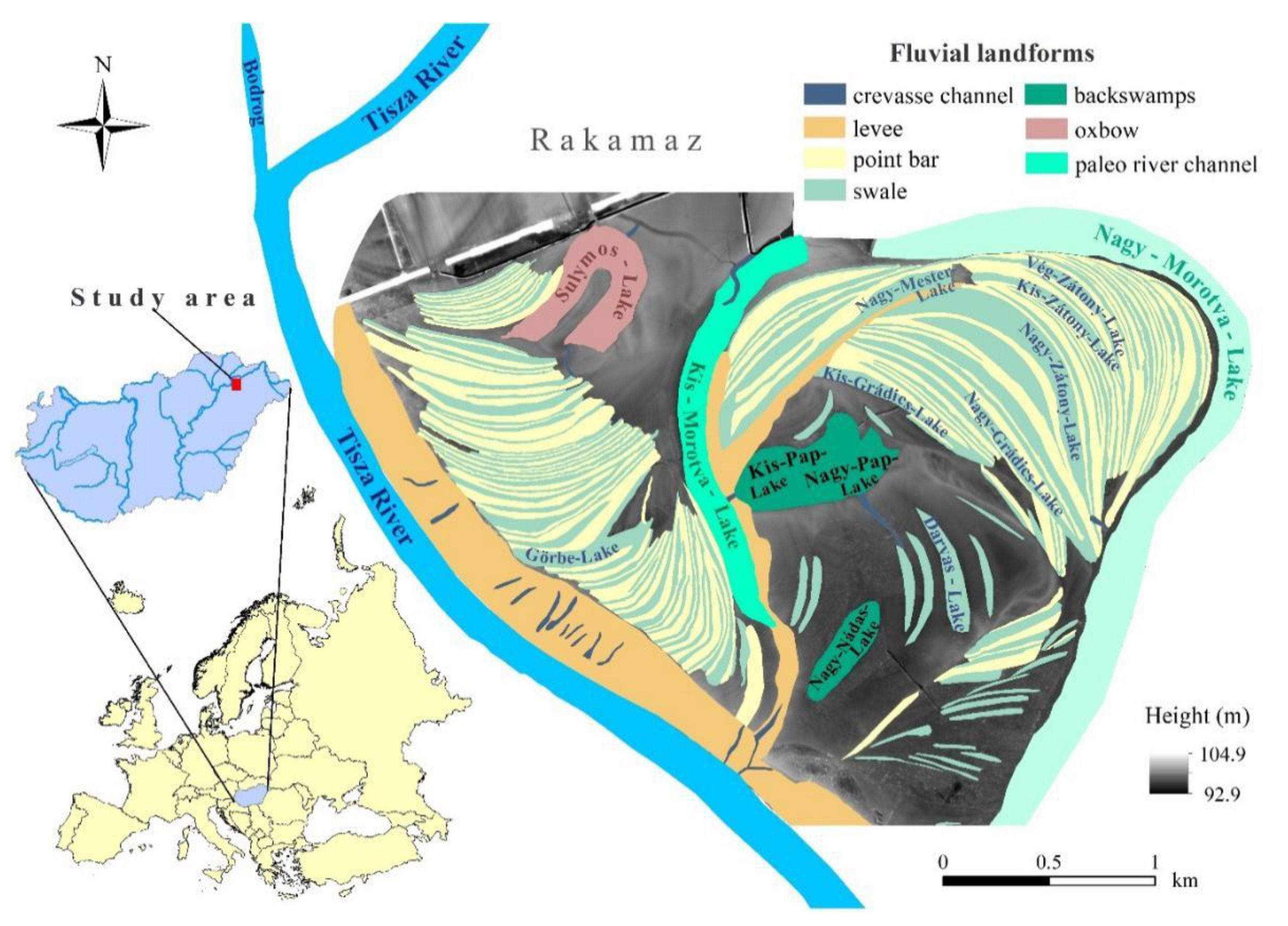
2.1. Study Site

Our study area is located in northeast Hungary, in the floodplain of the Tisza River below the confluence of the Bodrog River (Figure 1). The Tisza River becomes a typical plain-tract river here [48]. The study site extends over approximately 10 km2 and is very rich in fluvial landforms. Extensive farming activity is present here, which helps maintain the land close to its natural condition. The most typical landforms of the floodplain are scroll patterned landforms formed of point bars and swales left by the lateral migration of the Tisza River. They roll off the floodplain and make its surface wavy. Some of them are still very conspicuous, while others are rusty or filled in, making the differences between the forms faint. Some deeper and wider swales contain wet and marshy parts and dense aquatic vegetation, while others do not. The point bars are mostly without water and dense vegetation, expect in rare cases in which they are situated in a relatively low part of the floodplain. Solitary trees and groups of trees are present in both forms. An extensive levee lies next to the Tisza River, its surface dissected by natural crevasse channels at many points. This levee is used as arable land. A less conspicuous levee is situated next to a paleo river channel. Two backswamps and an oxbow lake can be also found on the study site. There are artificial crevasse channels between some forms to help the movement of water. Some forms had been already delineated and labelled (e.g., oxbow lake: Sulymos-Lake, paleo channel: Kis-Morotva-Lake, swale: Nagy-Zátony-Lake) in the Hungarian national 1:10,000 scale topographic maps.

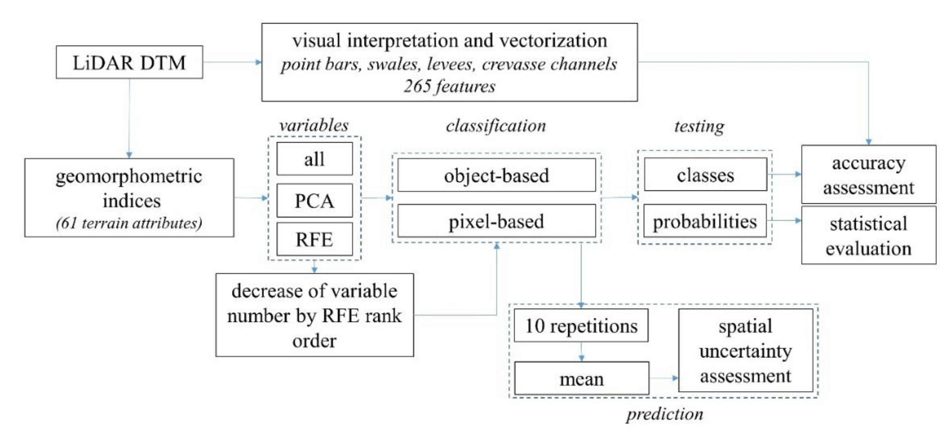
2.2. Data Set and DTM Generation

The aerial survey of the study area was carried out by a Riegl LMS-Q680i aerial laser scanner in the framework of the SH/2/6 program in August 2012 [49] by Envirosense Ltd. The predetermined point density was 4 point/m2, and the accuracy was ±15 cm both vertically and horizontally. Our base dataset was the point cloud provided by the Trans Tisza Water Directorate. We conducted noise reduction with the neighbourhood distance based method and ground point classification with Cloth Simulation Filters (CSF) [50]. The DTM was generated from the ground points with the Natural Neighbour interpolation method at a resolution of 1 m with 0.18 m RMSE (Root-mean-square error) in the ESRI ArcGIS 10.3.1 software environment [51].

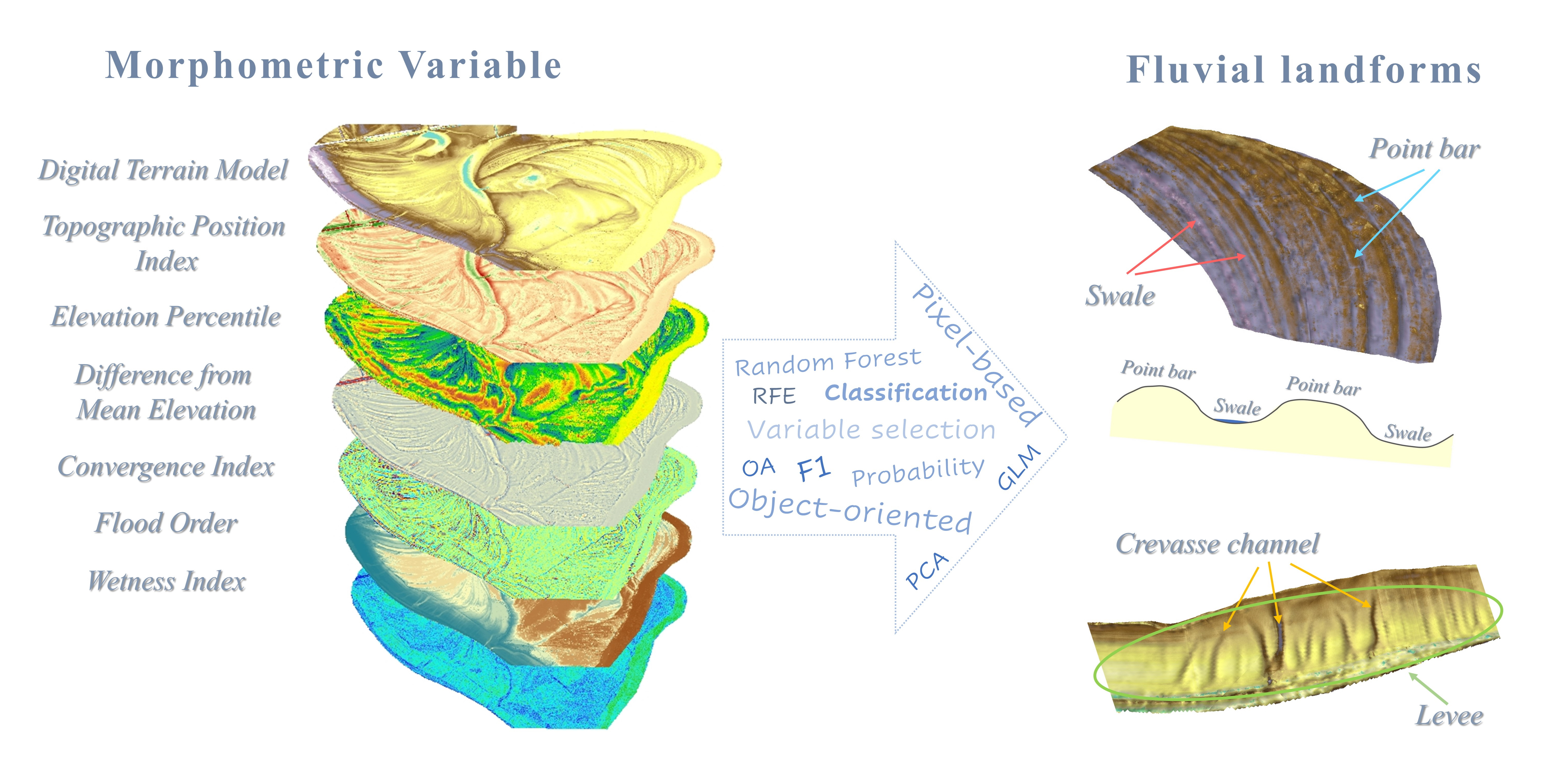
2.3. Terrain Analysis

We conducted a geospatial analysis with two open access software programmes, SAGA GIS (System for Automated Geoscientific Analyses Geographic Information System) 6.3.0 [52] and Whitebox GAT (Geospatial Analysis Tools) 3.4.0 [53] and we determined 60 terrain attributes from the DTM including basic parameters such as aspect, slope, gradient, curvatures, and secondary attributes such as the wetness index, the multiresolution index of valley bottom/ridge top flatness, mass balance and the convergence index (Table 1). Furthermore, there was an opportunity to use algorithms to determine the flood order for each of the cells within the DTM and to carry out elevation residuals analysis [53]. Some terrain attributes had tuning parameters; thus, in these cases, we repeated the calculations with different settings (e.g., difference from the mean elevation tool with 8, 16, 32 search neighbourhood sizes) to find the most suitable one for the characterisation.

2.4. Preprocessing of Input Data for Model Building

The first step was to develop a geomorphology map of the fluvial forms of the area; such a map was generated in our previous work [47] by visual interpretation of available aerial photos and the DTM combined with field mapping. The map was edited in the GIS environment and was the input database of all analyses with 265 geomorphological features (105 point bars, 127 swales, 20 crevasse channels, 13 levees; the 2 levees of the study site were divided into subsections to ensure more features were included in the analysis).

2.5. Model Building

2.5.1. Variable Selection

As 61 (the DTM and its 60 derived attributes) variables cause serious issues regarding overfitting, we intended to reduce the number of predictors; accordingly, we applied the Recursive Feature Elimination (RFE) technique. RFE was used directly with the classification algorithm (in our case with the Random Forest) based on the following theory: variables with the least contribution to overall accuracy are omitted from the set of predictors through iterations. Thus, the initial model considers all predictors and after removing one variable the model is rebuilt and run again. This process lasts until only one variable (with the largest contribution) remains in the model. Finally, the result is the rank of predictors based on their importance in making a contribution to obtaining greater classification accuracy [76]. We applied the RFE with a 10-fold cross-validation with 3 repetitions in R 4.03 with the caret package [77].

2.5.2. Supervised Classification Procedure

Random Forest (RF) is a robust and popular classifier in the remote sensing community because it does not make assumptions on normal distribution and variance homogeneity but its classification performance is high [78,79]. RF, as a classifier, has proved its efficiency in satellite imagery based land use studies [80,81,82], in urban studies based on aerial photography [83] and even in geomorphological object identification using DTMs [84,85]. Accordingly, we also chose RF as a supervised classification method.
Having the rank of predictor variables derived from RFE, i.e., knowing the predictor-set of the optimal predictor variable number that ensures the highest overall accuracy, we conducted model runs involving a decreasing number of variables with the RF classification. We removed one variable at a time with the lowest contribution until only one variable remained. We applied 500 trees, as earlier studies reported that errors stabilize before 500 trees are achieved [86]. Furthermore, the mtry parameter (the optimal number of variables for splitting at nodes) had been optimized to obtain the greatest accuracy: models were run with increasing mtry values from 2 to 30, and the best model was chosen based on the highest Overall Accuracy. All models were run with a 10-fold cross validation with 3 repetitions. This may seem redundant with the RFE; however, the result was an optimized model that can also be used for prediction, which was applied in the uncertainty analysis.
We aimed to identify swales, point bars, levees, and crevasse channels as the most frequent forms of the study area. Classification was performed with both (1) pixel-based (PB) and (2) object-oriented (OO) approaches (Figure 2).
  • We used the vector layer as reference data of the fluvial forms: stratified random sampling was carried out and we chose 5000 pixels for training and 5000 pixels for testing.
  • Polygons of the reference vector layer were used as objects; thus, the object-oriented term did not mean automatic segmentation, but real fluvial objects interpreted in a visual way. We determined the mean values of the DTM and the 60 derived raster layers by geomorphological features.
Both pixel sampling and mean value extraction were performed in ESRI ArcGIS 10.3.1 [51]. Classifications were performed in R 3.6.3 (R Core Team, 2020) with the rpart [87] and caret packages [77], and in EnMAP-Box (Environmental Mapping and Analysis Program) 2.1.1 software [88].

2.6. Model Evaluation and Uncertainty Analysis

We used the geomorphological map (see Section 2.4) as the reference dataset: in the OO-approach, the dataset was randomly split into training and testing, in a 50–50 ratio; in the PB-approach, we generated a stratified random sampling with 10,000 points within the polygons of the forms, split randomly into 5000 training and 5000 testing datasets.
We determined the Overall Accuracy (OA) as a general index of classification performance (Equation (1), [89]), and the F1 [90] for each class (Equation (2)).
OA = (TP + TN)/(TP + TN + FP + FN)
F1 = (2TP)/(2TP + FP + FN)
where TP: true positive, TN: true negative, FP: false positive, FN: false negative number of classifications.
While the OA provides a general evaluation of classifications and makes it possible to compare different model performances, the F1 is the harmonic mean of the Producers’ and Users’ Accuracy (UA and PA) [91], and evaluates the class level performance.
For the evaluation of model performances, we applied a 10-fold cross-validation with 3 repetitions (RKCV): the training dataset was divided into 10 subsets of which 9 were used to train a model and one to test it; in the next step, another 9 subsets were used to train another model and the remaining subset for testing. The process finished when all subsets had been used for testing; finally, the whole procedure was repeated with another two randomly selected subsets, resulting in 30 models. We reported the medians of the OAs of the 30 models, and each OA was calculated on the test data (i.e., independently of the training dataset).
Next, we calculated the OAs and F1s using the test dataset, and also the “out-of-the-box” accuracies using the training dataset for testing, which was important to determine the level of overfitting (see Section 2.8).
Beside the thematic accuracy, we also evaluated the probabilities: RF classifications rely on the highest probability assigned to the classes (in our case fluvial forms); thus, to explore the variation in the maximal probability, the values per form provide important information [92].
The RF algorithm uses random selection of input data for the numerous (in our case 500) decision trees in different model runs, thus, theoretically, models cannot be repeated, i.e., all models are different. However, R (and Python) software provides the possibility of a repetition with the same result (random sets should be defined). We performed the predictions with the optimized model with 10 different random sets. While repeated cross-validation produced 30 models, providing a thorough analysis using the mean, median, standard deviation, and interquartile range of each model, it only used the reference dataset.
A spatial analysis was performed with the predictions: we used the whole data of the study area and we calculated the uncertainty. We repeated the predictions with 10 different RF models with the models of different numbers of input variables (20, 15, 10, 9, 8, 7, 6, 5, 4, 3, 2). Then, we determined the mean values of the 10 predictions, and we expected the following coded landforms: 1 (as crevasse channels), 2 (as point bars), 3 (as swales) and 4 (as levees). If all predictions of the repetitions resulted in the same code, numbers would be whole and identical with the expected classes’ number, but if the prediction resulted in different morphological forms (i.e., classes), the mean would be a number with fractions. Thus, if we count the number of whole numbers where the results are fractions, we can visualize and express the level of uncertainty in the predictions.
Furthermore, beside the classifications, we also calculated the probabilities associated with the given pixels. R software provides the probabilities for each class and we combined the chosen class and the related probability to the reference pixels. Thus, we were able to evaluate the interaction of the class level probabilities and the effect of the number of variables.

2.7. Predictor Stability Analysis

Predictors, i.e., geomorphometric variables, were selected by the RFE variable selection method, but the selection is a function of the input data. Accordingly, we also studied the selected variables of the RFE. We had set 11 different random samples with 1000 pixels from the 5000 training pixels and, using the RFE with 10-fold cross-validation with 3 repetitions, we determined the rank orders of the 11 realizations and we then evaluated and summarized the rank orders by their frequency.

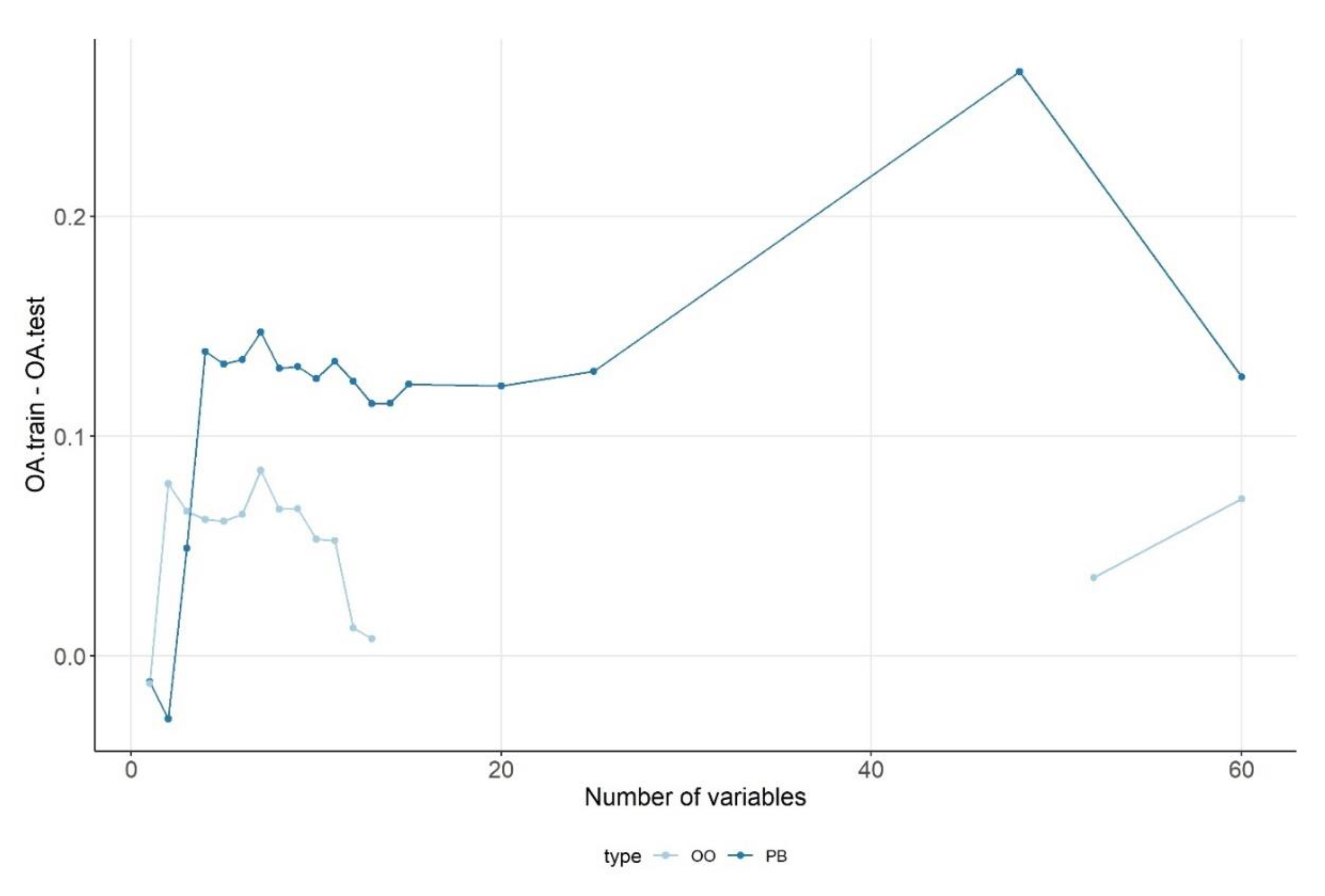
2.8. Analysis of Overfitting

As a measure of overfitting, we determined the OA, both with the training dataset (i.e., dependent on the model, OAtrain) and the testing dataset (independent of the model, OAtest). The difference between the two types of accuracies revealed whether the classification performance was the function of a large number of variables (Equation (3)).
Overfitting = OAtrain ‒ OAtest
where OA is the Overall Accuracy.

2.9. Statistical Evaluation

We determined the Pearson correlation coefficients among the geomorphometric variables and visualized the results in a correlation plot grouped by hierarchical clustering with the Ward method. Nominal variables had been omitted. The correlation structure’s internal consistency was quantified with Cronbach’s α. If all variables correlate, α = 1, and when variables do not have any correlation with the other, α = 0 [93]. We also determined α-values per variable, which helped to find the metrics that deteriorate the internal consistency.
We applied General Linear Modelling (GLM) to reveal the relationship among the class level accuracy measure, the F1, the type of fluvial forms (as factor) and the number of variables (as covariate) [94]. Assumptions were checked with the Shapiro–Wilk test (normality) and the Levene test (variance homogeneity). Partial contributions of the independent variables were reported with the effect size (ω2) [95]. Statistical analysis was performed in R 4.03 with the gamlj and corrplot packages [96,97].

3. Results

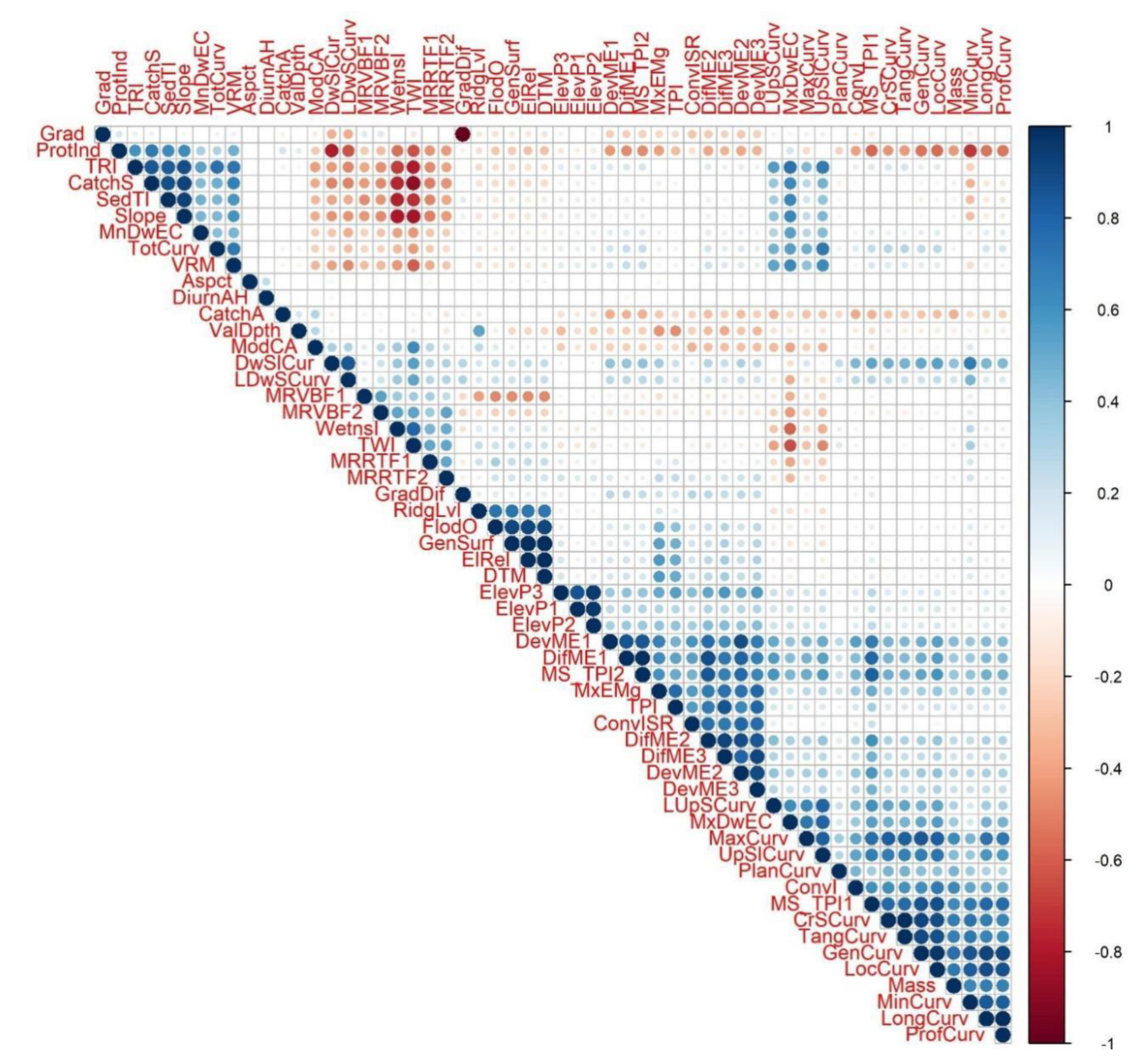
3.1. Results of Data Preprocessing

First, we conducted PCA (Principal Component Analysis) on the variables of the pixels extracted from the raster layers (PB-approach), which indicated a good fit (Root Mean Square Residual - RMSR = 0.05); however, the first five PCs explained only 73% of the total variance and several variables had poor (<0.5) community values. After excluding 11 variables (MnDwEC, Aspect, CatchA, DiurnAH, ValDpth, ModCA, MRRTF1, MRRTF2, PlanCurv, TotCurv, ConvI), the model fit was the same (RMSR = 0.05), but the explained total variance changed to 78% (Table 2).
Next, we repeated the PCA with the OO-approach (i.e., pixel means of the visually interpreted segments of fluvial forms). In this case, we also had to exclude variables due to low communality, although only three of them were excluded (MxEMs, DiurnAH, PlanCurv), and the explained total variance was 86% with good fit (RMSR = 0.04) (Table 3).
The correlation plot (Figure 3) also showed that geomorphometric variables formed highly correlating groups, but these groups usually contained 6–7 variables (i.e., corresponding to PCs of PCA). Cronbach’s alpha indicated poor reliability (<0.001), but the omission of FlodO, MxEMs, Aspct, CatchA, ConvI, ModCA and ValDpth resulted in a better outcome of 0.690. This value is still low; it should usually be above 0.8.
RFE revealed the most important variables, and according to the different numbers of data, and the different types of data collection (large number of cases vs. fewer aggregated data), the ranks were different:
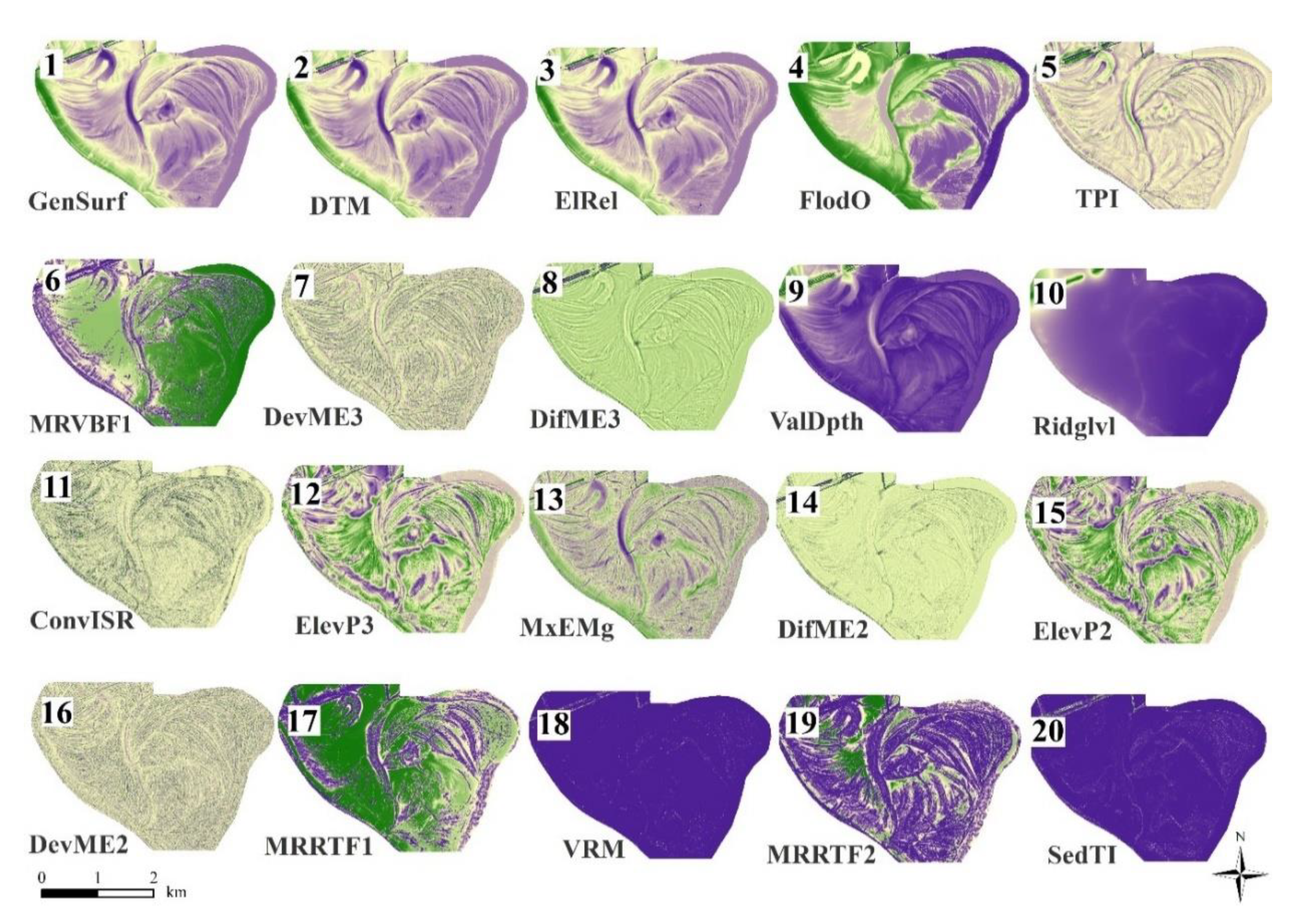
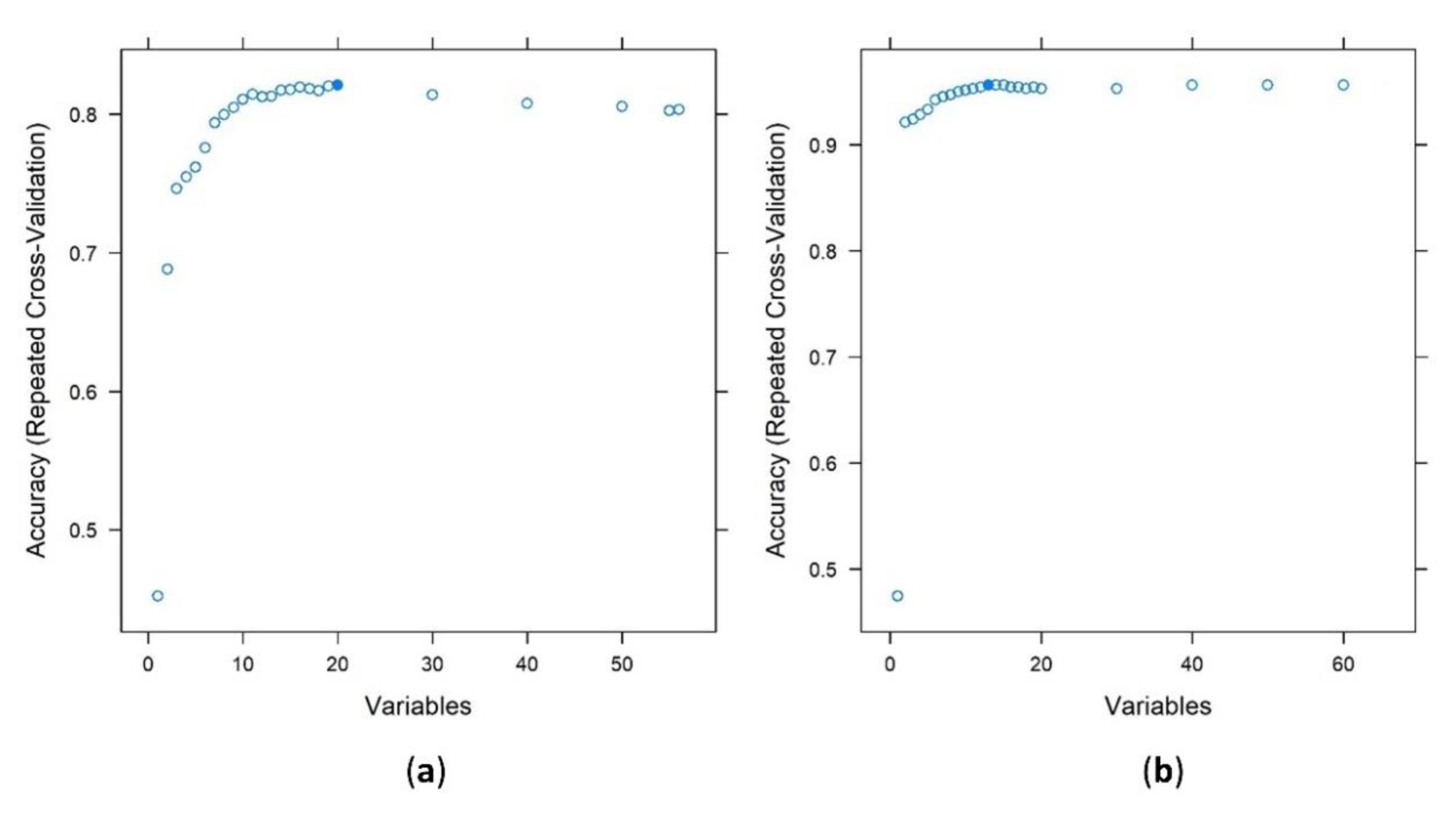
  • PB-approach: maximum OA had been reached with 20 variables (Figure 4) GenSurf>DTM>ElRel>FlodO>TPI>MRVBF1>DevME3>DifME3>ValDpth>RidgLvl>ConvISR> ElevP3>MxEMg>DifME2>ElevP2>DevME2>MRRTF1>VRM>MRRTF2>SedTI.
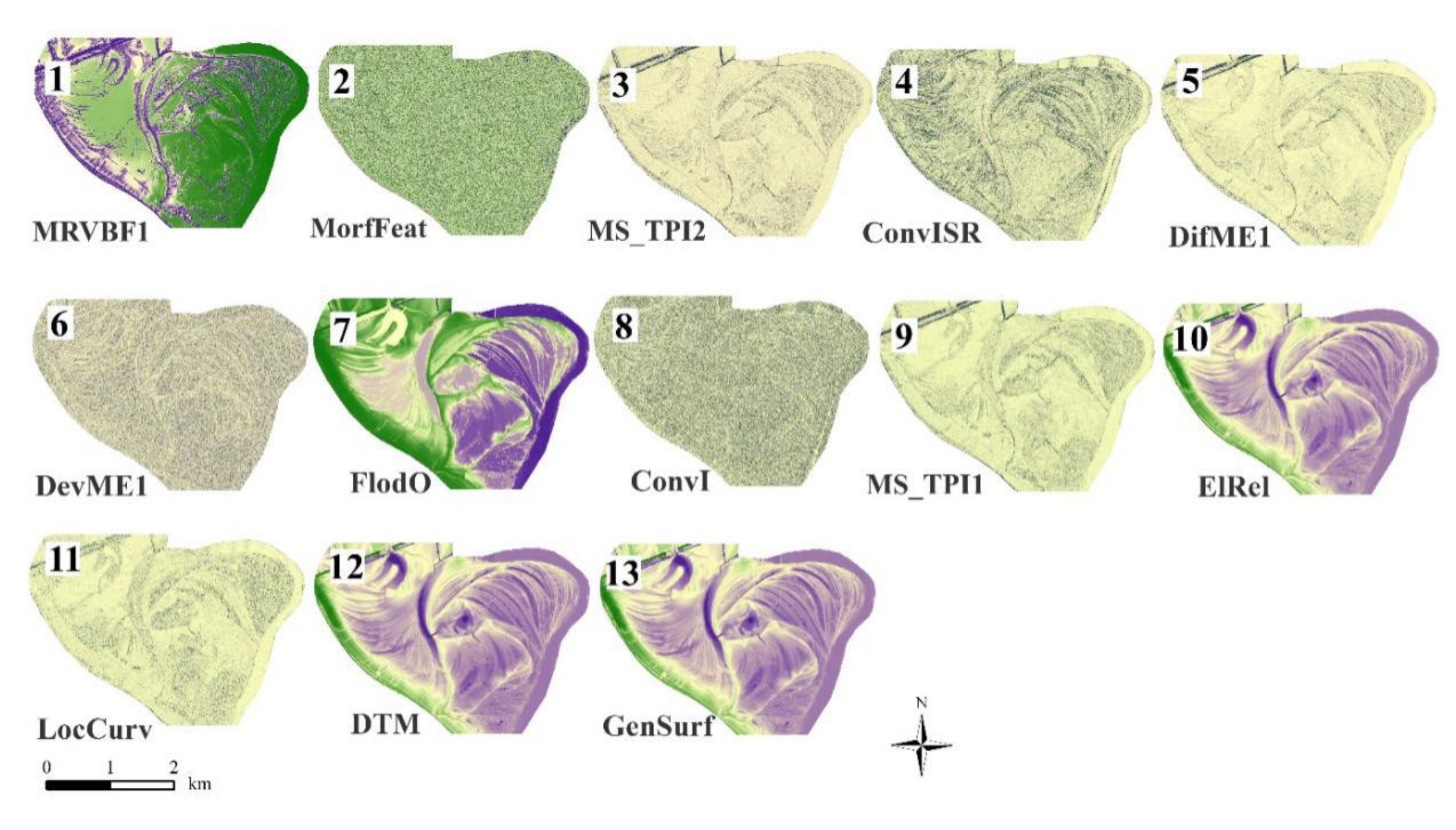
  • OO-approach: maximum OA had been reached with 13 variables (Figure 5) MRVBF1>MorfFeat>MS_TPI2>ConvISR>DifME1>DevME1>FlodO>ConvI>MS_TPI1>ElRel> LocCurv>DTM >GenSurf.
A stability analysis of the variables of the PB-approach according to the RFE showed that the number of optimal variables (i.e., ensuring the largest OA) varied between 11 and 20, and the OAs varied between 78.5% and 81.1% (Figure 6). GenSurf was the first in the rank order in eight cases out of the 11 repetitions, ElRel was the second in eight cases, DTM was the third in seven cases, FlodO was the fourth in eight cases and TPI was the fifth in five cases; all other rank places were mixed with different indices. Regarding the first ten variables, GenSurf, ElRel, DTM, FlodO, TPI, DevMe3, DifME3 and ValDpth were stable elements of the ranking, MRVBF1 was in the list in nine cases, and the rest of the places consisted of other morphometric indices.
The rank order of the variables was different for the OO-approach: the optimal number of variables varied between 10 and 60, with almost the same OAs between 95.2% and 95.7%. The most important variable was MRVBF1, which was the first in the rank order in 11 cases of the 11 repetitions. The second in the list was MorfFeat in 11 cases, the third was ConvISR in 5 cases, the fifth was MS_TPI2 in 8 cases and the sixth was DevME1 in 11 cases. From the seventh place in the rank, there was no dominant variable.

3.2. Overall Accuracies of RF Classifications

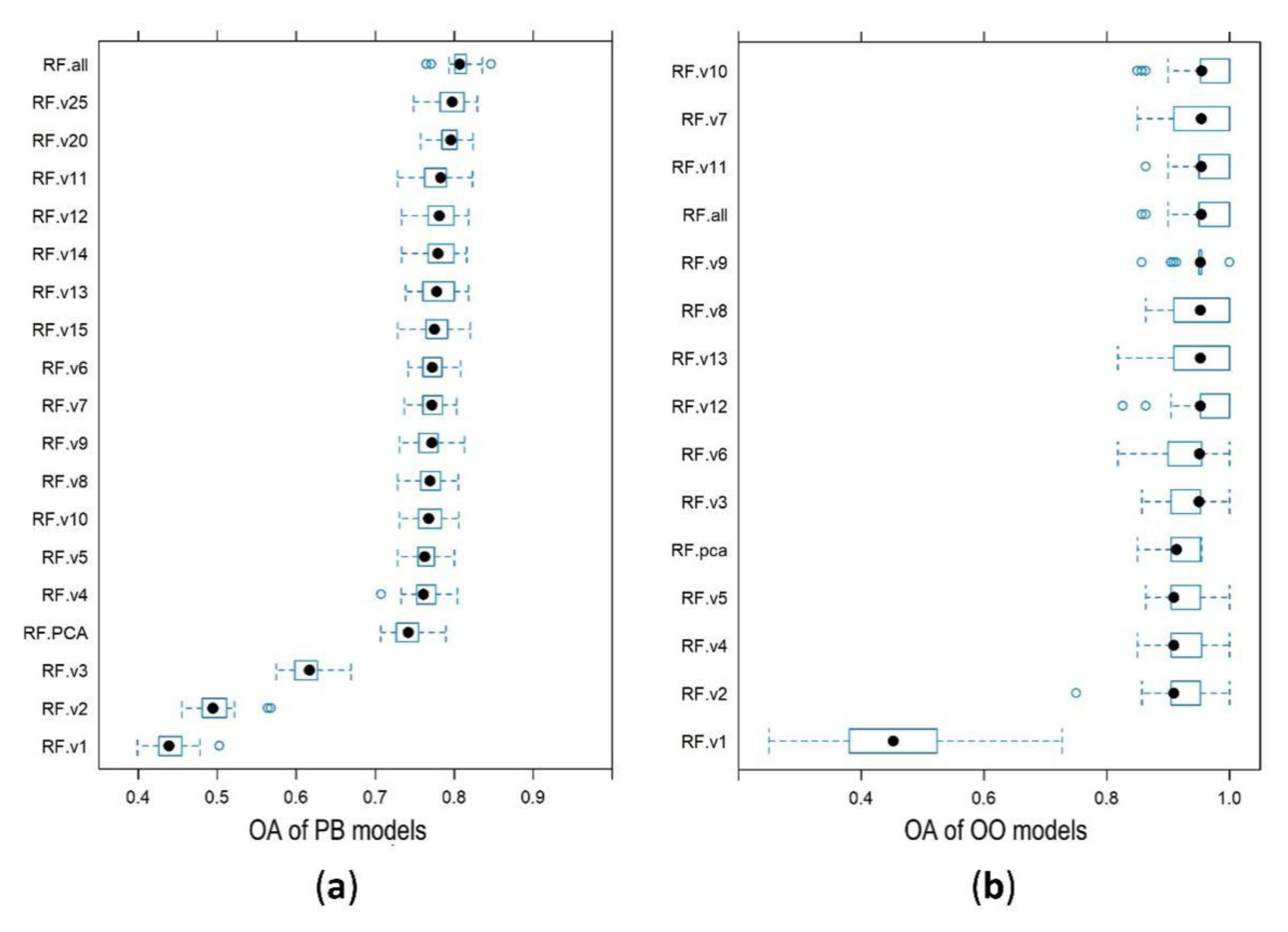
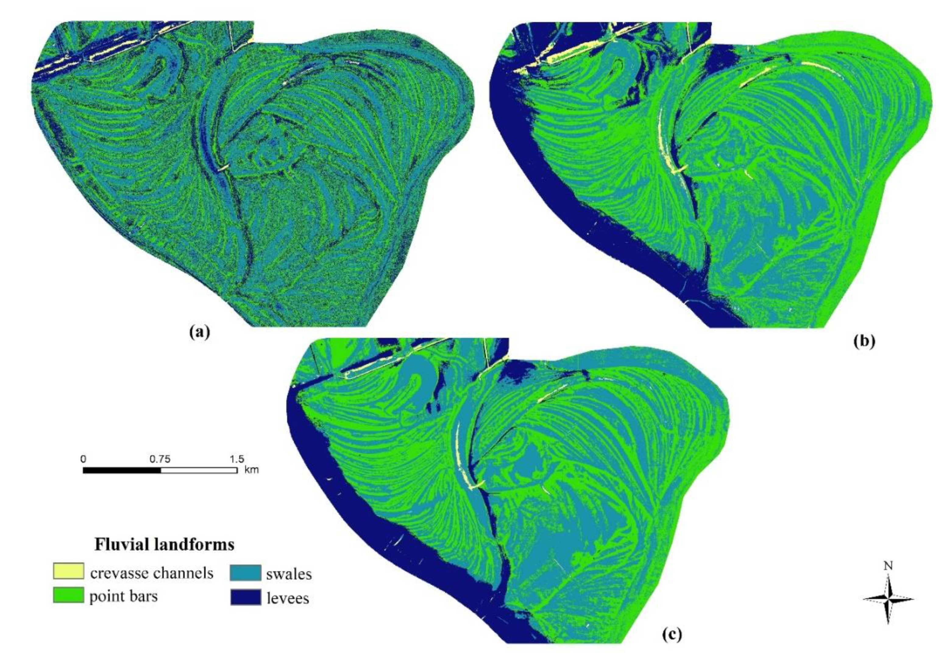
3.2.1. Pixel-Based Classification

As a first step, we involved all of the 61 variables and determined its overall accuracy: its 80.7% median OA indicated an efficient outcome (Figure 7a). Reducing the number of variables caused a slight decrease in OAs, but the rank order by OAs did not follow the number of variables. Differences in the OA-medians were slight and ranged between 79.7% (25 variables) and 76.1% (four variables). The model with four geomorphometric indices, GenSurf, ElRel, DTM and FlodO, was only 4.6% worse in the prediction than when 61 variables were used (Figure 7a and Figure 8b). Furthermore, 11 variables resulted in the fourth best result (78.3%), and the optimal 20 variables according to the RFE produced an OA of 79.5%, which is only 1.1% worse than the model run with 61 variables. Finally, we tested the efficiency of the PCA-model, which was the fourth worst model (with a median of 74.2%), and worse than using four variables. However, there was a threshold in the decrease in OAs at three variables: the decreases in the OAs changed from <1% to 15%.
Visualizing the classifications revealed that the 2-variable solution relevantly underestimated the swales and had a high proportion of salt-and-pepper errors (Figure 8a). The appearance of the 4- and 20-variable versions showed clarified maps with only a small proportion of salt-and-pepper errors. Both versions had errors in the southern part of the study area; swales had been over-represented. However, this area consisted of lakes (Kis-Morotva Lake, Kis-Pap Lake and Nagy-Pap Lake) and a floodplain depression of an irregular shape. Further sources of misclassifications were also outside the areas of interest; these were oxbow lakes at the northern part (Sulymos Lake) and on the eastern border (Nagy-Morotva Lake). Generally, the 20-variable solution reflected the geomorphology in an acceptable way and all larger errors were any of the forms we intended to identify.

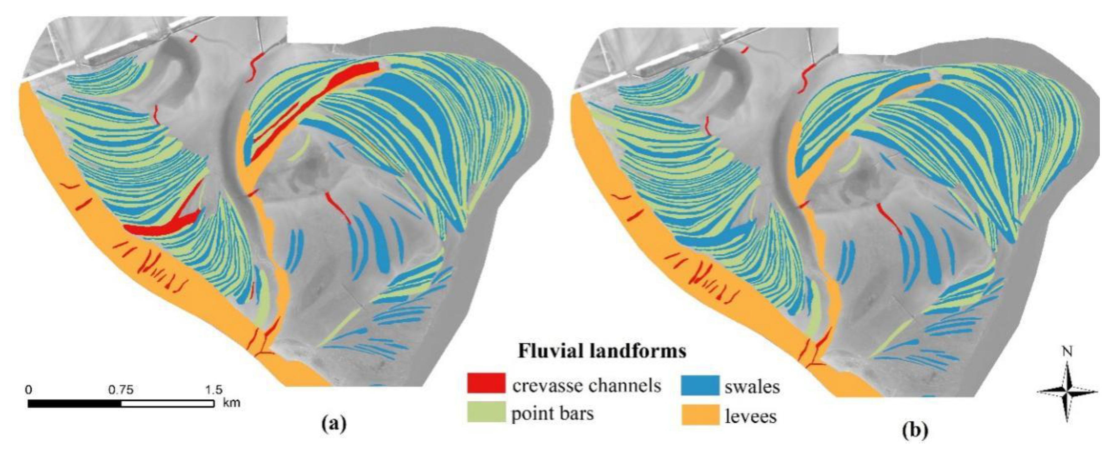
3.2.2. Object-Oriented Classification

We applied the same procedure in OO-based classifications, too, and the result was different: the best OA belonged to the model of 10-variables (95.4%) (Figure 7b), which is almost 15% better than in the PB-approach. Another difference is that the optimal number of variables was 13 according to the RFE variable selection, but it was only the seventh best model in the list. We can discriminate three groups by the OAs: in the first group, the OAs were between 95.4% and 95.0%, in the second group between 91.3% and 90.9%, and third group consisted of only one model (with one variable) with an OA of 45.2%. The first three variables, MRVBF1>MorfFeat>MS_TPI2, ensured a relatively high (95.0%) accuracy. Although the interquartile ranges were larger than in the PB-approach, even the minimums were ~10% higher in the OO-models.
Maps of the OO-approach, i.e., the classified polygons, did not have large differences regarding the number of involved variables (Figure 9). Related to the 13-variable model, the 2-variable model had only some misclassifications, the two models were very similar, and most of the differences were of swales wrongly classified as crevasse channels. Furthermore, we found swales classified as point bars, and a point bar classified as a levee, but the geomorphic characteristics had been well represented in spite of the model errors.

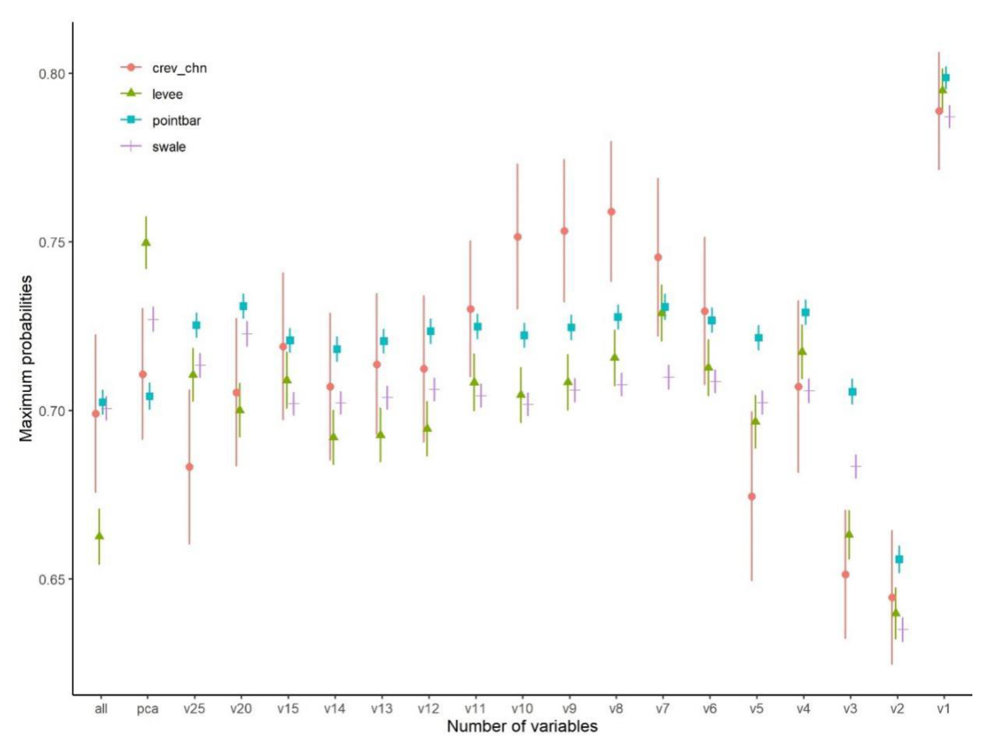
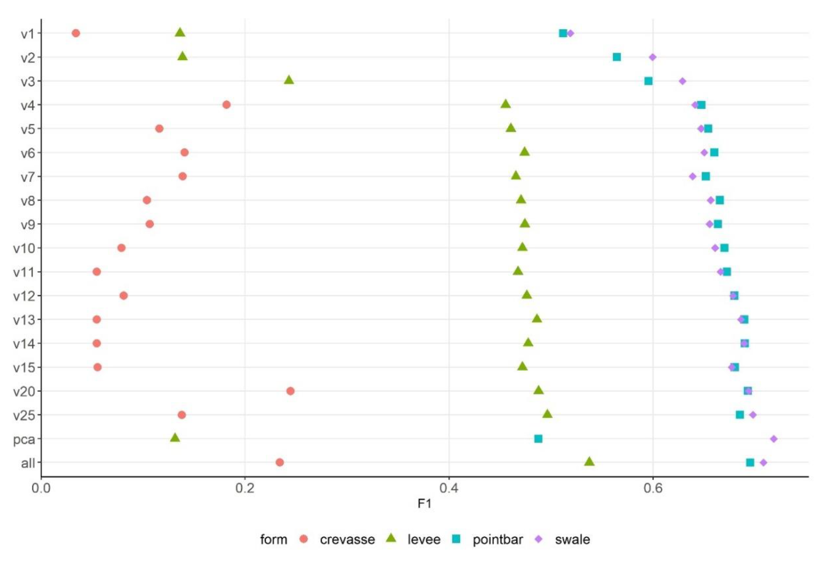
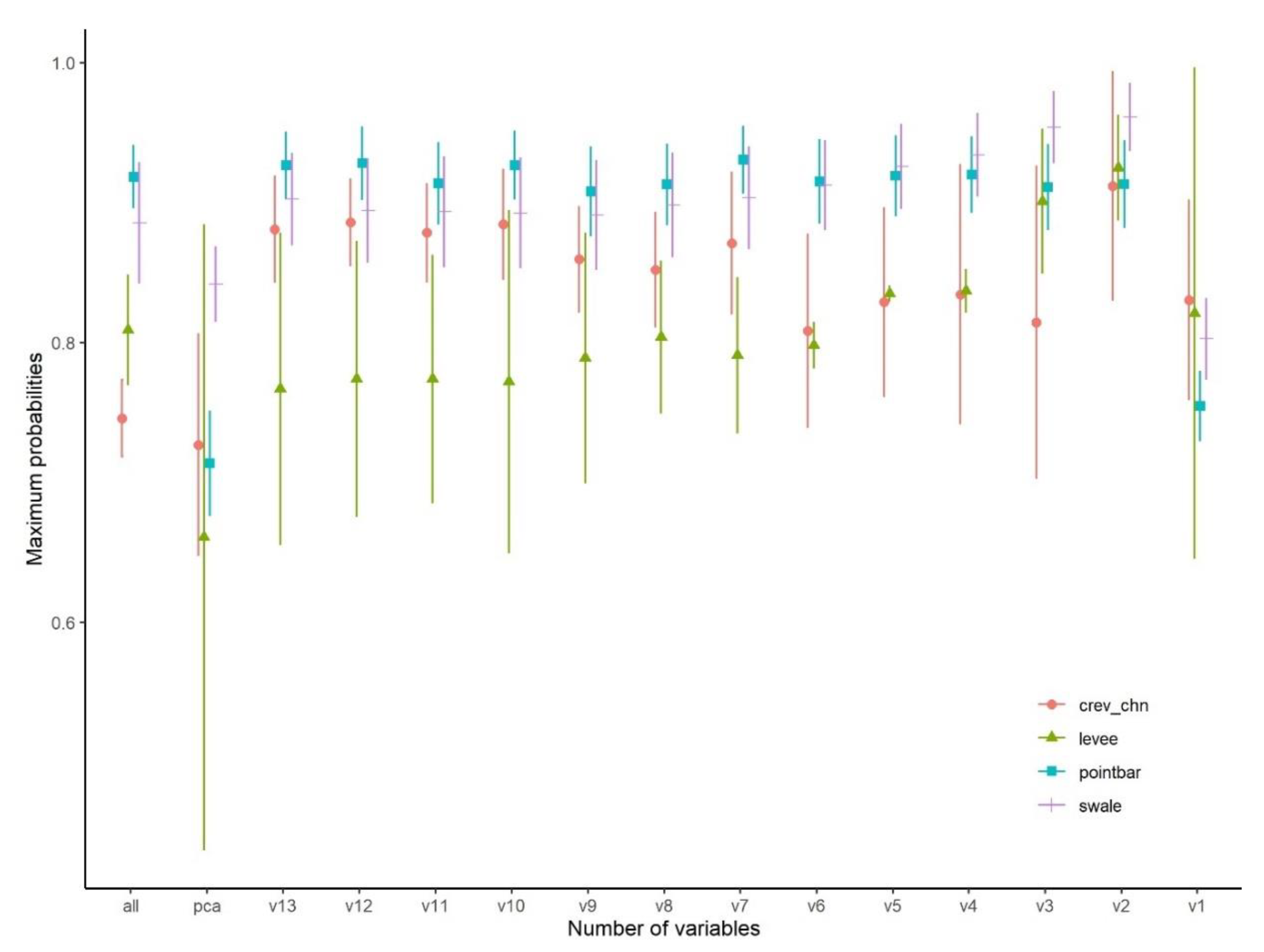
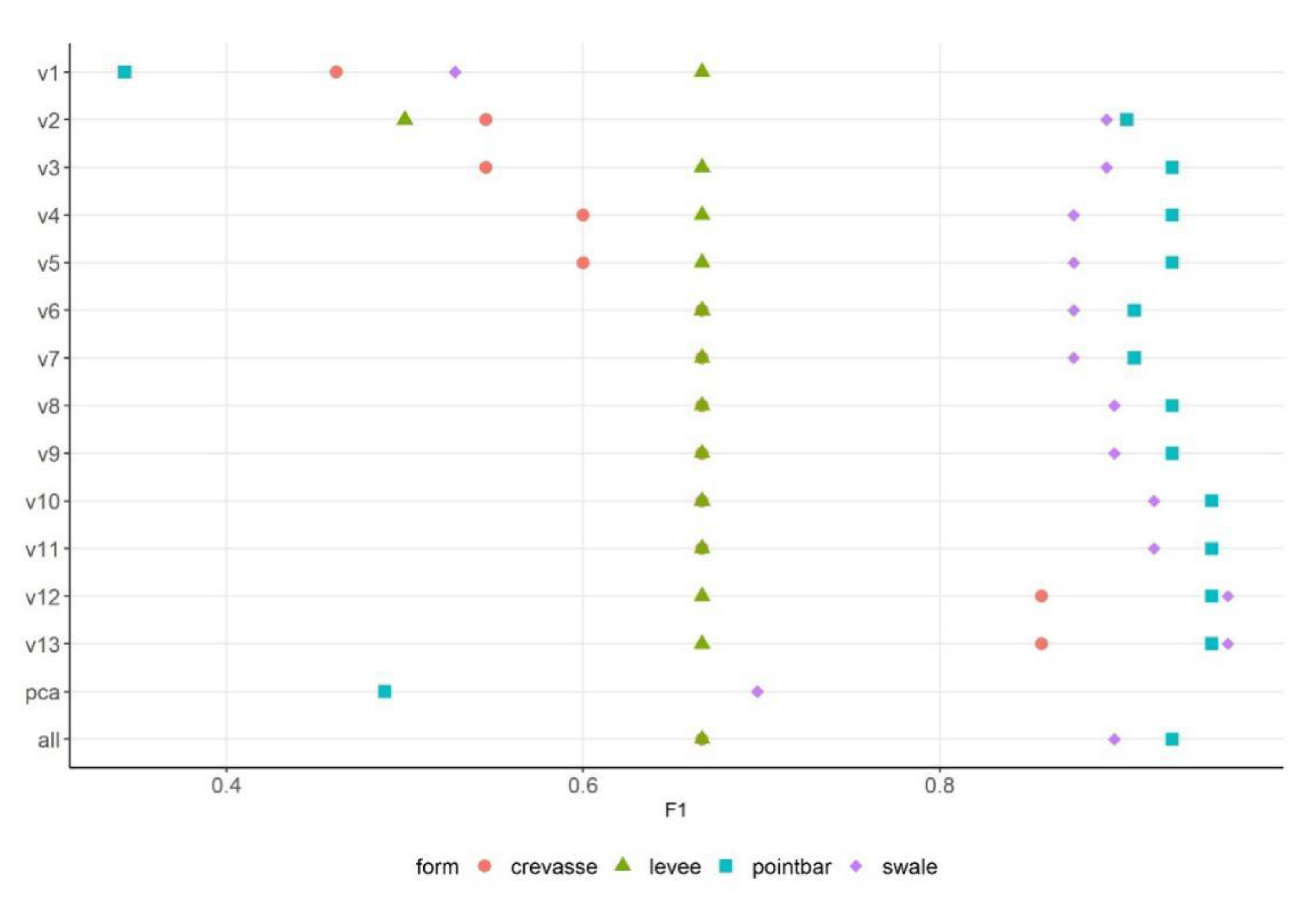
3.3. Class Level Probabilities of Classifications

The highest probabilities usually belonged to crevasse channels and point bars, while the lowest belonged to swales (Figure 10). However, this result is misleading, because F1-values indicated that the lowest accuracies were experienced in crevasse channels (<20%), and the swales and point bars had the greatest accuracy (60–70%; Figure 11). Regarding the number of variables, using 20 variables should have resulted in the most efficient model with the PB-approach according to the RFE, and this was true for the OA values (25 variables was only 0.2% better; Figure 6), but in the case of class level probabilities, the highest numbers were experienced with the 8–10-variable models, which were also efficient with the F1-values (Figure 11).
Visualized maximum probability values (Figure 12) correspondent with the maps, but this was a natural phenomenon as the result of the classification, and the probability had been calculated with the same algorithm and settings. However, combining this information with the mean values of the landform classes (Figure 10), we were able to justify that the spatial distribution of the different values of probability provided the landform map itself.
In the OO-approach, probabilities were higher, usually above 80%, and the levees had the lowest and the point bars the highest values (Figure 13). Although the 13-variable model did not result in better classification probabilities for the fluvial forms, the F1-values showed that the best class level performance belonged to this model (Figure 14). We also have to note that the performance of models conducted with 10–11–12–13 variables was almost the same according to the F1.

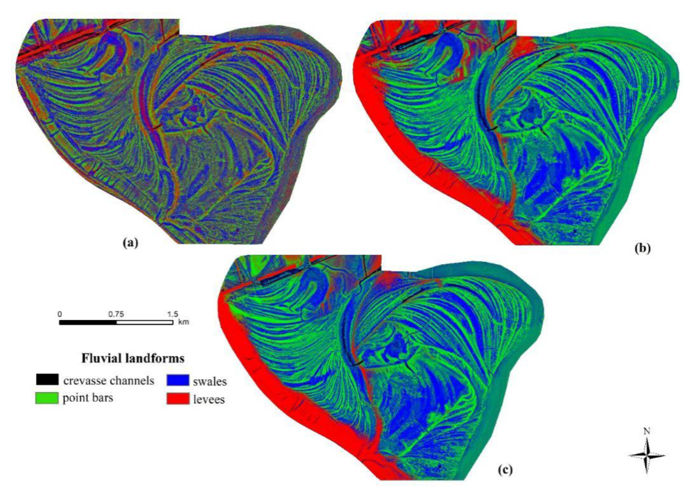
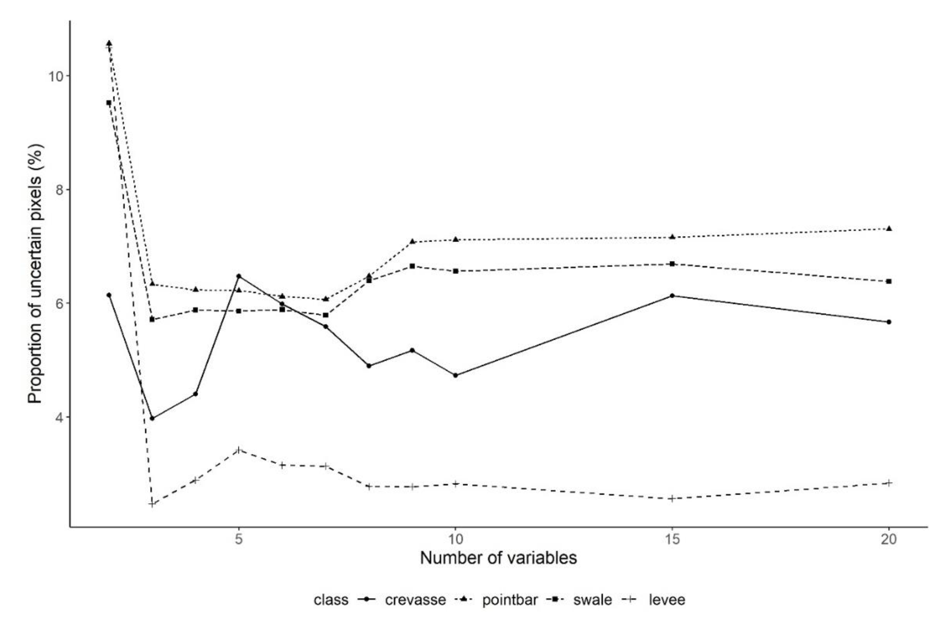
3.4. Spatial Uncertainty Issues

Spatial uncertainty analysis, as reflected in different realizations of classifications, also pointed to the fact that even a high classification performance showed different results, i.e., repetitions resulted in different spatial outcomes (Figure 15). According to the 10 repetitions, the lowest proportion of differing realizations was associated with the levees (mean: 2.8%), and the point bars and swales had the largest proportion with almost the same values (mean: 6.9 and 6.5%, respectively). The uncertainty was the highest with the 2-variable models, and became stable when more than 10 variables were involved, but this did not mean lower values: point bars and swales had 1% more uncertainty with 10 variables (increasing from 6.1 to 7.1%).

3.5. Result of Overfitting Analysis

Overfitting, i.e., the effect of the number of variables on the OA values, was not obvious: the overfit difference was usually more than 12% above four variables for the PB-approach and 7% with the OO-approach (Figure 16). However, the peak of the PB-approach at 48 variables (26.6% difference) belonged to the model using the PCs of PCA, and as we pointed out, the explained variance of the PCA was not high (only 78%). In the OO-approach, the explained variance of the PCA of 52 variables was higher (86%) with a better model fit, and the difference was one of the smallest. The analysis revealed that using all variables did not cause a larger difference between the OAs of training and testing datasets than using only five variables. In the OO-approach, the difference was the smallest with the 1-variable and the 13-variable models.
GLM models also indicated that F1 values were determined by the fluvial forms and the role of the number of variables was not significant, and also had a low effect size (Table 4 and Table 5). Accordingly, fluvial forms had characteristically higher or lower F1 values, i.e., the number of variables did not improve the class level indices in a relevant way.

4. Discussion

3D point clouds of LiDAR are considered to be the most efficient and powerful surveying method, which provides accurate data about the ground and objects’ surface height, even in vegetated areas. However, this data type can have issues in areas where the terrain is flat, but the relative differences cause important changes in the environment. These areas include wetlands, floodplains, and salt-affected steppes where 0.1–0.2 m relative differences cause changes in the water supply, soil moisture or salt content. A better understanding of the geomorphology and the fluvial processes can help sustainable planning in these areas, and the LiDAR technology can be a promising tool for this.

4.1. Object-Oriented and Pixel-Based Classifications

The OO-approach provided ~15–17% better model performance for fluvial form identification than the PB-approach. The object-based and pixel-based comparisons usually proved that segments ensure better input data than pixels. The authors of [98] came to the same conclusion; they applied object-based “geons”, i.e., homogenous regions, and pixels in the landslide susceptibility mapping and the approach using segments—the geons—provided the highest accuracy. Several other authors found the same results: [99] with hyperspectral data, [100] with Sentinel-2 images, [101,102] with ASTER images, and [103] with visible aerial imagery. We emphasized that our OO-based approach was not a classic segmentation of object-based image analysis (OBIA); our objects were fluvial forms interpreted by visual characteristics and field observations. Thus, in our case, one object meant a given fluvial form, with the sole exception of levees (there were too few forms: we divided up the existing ones to increase the cases). Similarly to the studies where OBIA was successful, our objects of fluvial forms were good basic units of the landscape, but the main difference from the OBIA lies in the interpretation: it needs expertise (the capability to identify the forms in aerial images, in digital terrain models and in the field); furthermore, it is time-consuming (depending on the extent), i.e., all objects in the area should be identified correctly; however, when it is completed, the geomorphological aspect is ready, too. Unlike segments that varied in shape as the pixel values changed, our objects covered all of the pixels that are characteristic of the classes. Accordingly, the mean pixel values of the raster layers of geomorphometric variables can regarded as the quantified measure of the separability of the forms. If classifications produce only a weak performance, we cannot expect a high degree of accuracy in the PB-approach. As our OO-based classifications provided about 95% OA, this was the theoretical maximum for the PB-approach, too. The 78–80% OA for the PB-approach was higher than using only the slope, aspect, terrain height and NDVI with two fluvial forms (71% OA; [47]).

4.2. Variable Selection, Number of Variables and the Issue of Overfit

Variable selection is a key step to reduce the number of variables in order to decrease the chance of overfitting while preserving high classification accuracy. We ran several models with different variable sets and the number of variables, and the results showed that in the OO-approach, the OAs were ~95%, and in the PB-approach, ~78%. The highest OAs were obtained with the highest number of variables for the PB-approach, but in the OO-approach this was not entirely true: involving all variables only resulted in the fourth place (although it is also important that the difference among first three models was <0.2%). Accuracy assessment using the RKCV was 7% worse than testing with the training data, indicating serious overfitting. With the OO-approach, the smallest overfit was experienced with the 1-, 12- and 13-variables models (1%, 1.2% and 0.8%, respectively). The overfitting was 6–7% in all other models, regardless of the number of variables, and even when using 2–9 variables. In the PB-approach, the overfitting was higher, at 11–12%, and the lowest values were observed with 1–3 variables. However, 1–3 variables produced a poor model performance, too; thus the lowest overfit values were not useful in selecting the best model.
An uncommon phenomenon was experienced with the PCA: application of PCs usually results in higher model performance, as has been proven in different studies [104,105,106,107]. However, in this case, the PCA was not a successful alternative. According to the analysis of correlation structure, several potentially useful metrics should be omitted based on the communality and the item-related Cronbach’s α. For example, FlodO, ConvI and ValDpth were important predictors in the classification, but if we insist on the correlation-related dimension reduction, we have to miss them. The reason was that the correlation structure was not optimal, and the variables were geomorphometric indices and not bands of a hyperspectral sensor, where there is a high level of correlation between the bands. The authors of [108] used PCA with geomorphometric variables in watershed prioritization, but they used watershed parameters, which resulted in a better correlation structure. The authors of [109] used PCA to reduce 230 terrain attributes to 67, and they concluded that five metrics were enough to explain 51% of the total variance. In our case, we were not able to delineate this reduction, but the RFE as a feature selection method was appropriate to find the most important variables.
RFE provided a list of 13–20 variables from the possible 61, but the structure, i.e., the variables that make the list, varied. RFE was run with the RF algorithm, which uses several decision trees of bootstrapped samples, and all model runs can provide different results. Our experiment with 11 randomly selected datasets from the 5000 pixels and 265 forms showed that the OO and PB-approaches had different variables that contribute to the highest OAs. Furthermore, there were important variables, with relevant contributions in all repetitions. Our third observation was that although the variable sets could differ in the repetitions, the OAs obtained were the same in 1–2% variations. Accordingly, if there are many variables, there are different variable sets, which ensure more or less the same result. The most important geomorphometric indices were GenSurf, ElRel, DTM, FlodO, and TPI for the PB-approach, and MRVBF1, MorfFeat, ConvISR, MS_TPI2, and DevME1 for the OO-approach. In the first most important ten variables we find overlaps, but with different settings, i.e.,: with DevME and DifME, although MRVBF was the same regarding the ranks. Differences in the importance were normal, because the number of the data (1000 vs. 265) and the characteristics of the data (pixel values vs. pixel means by forms) were also different. The authors of [110] pointed out that RFE is useful in reducing predictor numbers; thus, machine and deep learning algorithms can be faster without variables that make a small contribution. We also experienced that RF models were trained in a shorter time, and the model accuracy was only slightly (1–2%) lower; moreover, in the OO-approach, omitting irrelevant predictors, and with only 10–13 variables, the model became ~1% better.
DTM (absolute terrain height) should have been efficient alone, but as the terrain had a slight change from the river to the dyke, and from the North to South, thus, swales and point bars can have the same height in the area. Accordingly, the most efficient metrics were able to reflect the specific characteristics of fluvial forms, i.e., the shapes, convexity–concavity, and relative situation of the forms. Efficient variables considered the relative differences (based on minimums and maximums) of the neighboring areas; furthermore, the convergence–divergence, GenSurf, Elrel, FlodO, MRVBF1 and ConvISR were important both for PB and OO-approaches, while DevME and DifME were also important but with different settings: the larger kernel window (with 16 and 32 neighboring pixels) were efficient for the PB-approach and the smaller kernel (8 neighbors) had large importance for the OO-approach. Finding the right class of a single pixel requires larger neighboring area, while with the OO-approach values belonging to objects are means of the given polygon; therefore, larger kernels mean double averaging and do not help the classification.

4.3. Uncertainty

We measured the uncertainty in different ways, and the results were contradictory. The highest probability was associated with the classification, and highest values indicated that the decision regarding the classification was made in a straight or an ambiguous way, e.g., if the given probabilities varied, for example 0.90, 0.05, 0.05, 0.00, this meant that the classification identified the first class as 90%, but if this occurred for another form the values were 0.40, 0.35, 0.25, 0.10, which meant that there was only a 5% difference between the first and second classes. Based on this, we expected that higher probabilities would cause better classification accuracy on a class level, but there was no connection between the mean probabilities of fluvial forms and the F1s. Moreover, there were contradictions in the PB-approach; the correlation was 0.14 with the highest probabilities associated with the crevasse channels, whilst the F1s were the lowest (even <10%). Although the results were more similar with the OO-approach, the correlation was 0.74, and contradictions were also found (crevasse channels also had high values in some cases with low F1 values). Nevertheless, probability values reflected the spatial distribution of the landforms: all forms can be delineated based on the maximum probability of the pixels. This means that the maximum values differed by class, and these values were characteristic for all pixels of a given class. However, this value did not correspond with accuracy.
Spatial uncertainty analysis also produced similar results: the proportion of uncertain pixels was the highest for swales and point bars, and the lowest values occurred with the levees; meanwhile, the class level F1s showed the opposite result: swales and point bars had the highest class level accuracy. Considering the dominance of these two forms in the area, there is also a higher chance of misclassifying them. Point bars and swales have similar shapes and the main difference between them is that swales are concave while point bars are convex forms [47]. Swales are shallow and elongated depressions with varying water cover or at least higher soil moisture, the vegetation is denser, and tussocks (Carex species) form a naturally uneven surface. Thus, considering that the terrain height has a tendency to increase from the river to the dykes, all swales differ in extent, water cover, vegetation cover, and absolute height above sea level. Point bars can have the same terrain height as swales and in certain locations (i.e., lower point bars between higher point bars) and at certain time can be covered by water; thus, they can also have denser vegetation related to those in a higher terrain position [50,111]. Although these forms can be discriminated easily with visual interpretation, and can be identified in the field by geomorphologists, due to the large number of forms combined with the similarities, semi-automatic misclassification between these two forms can be regarded as normal.
All classifications have errors, and similar features are hard to discriminate. The fluvial forms of a floodplain have similar geomorphometric properties; thus, even with the most accurate aerial LiDAR-based DTMs, classifications cannot be accurate. Using the objects’ outlines and calculating the mean pixel values by raster layers (i.e., the OO-approach), very accurate 95% models can be obtained, but this supposes that there is a properly interpreted map of the morphological forms. However, the accuracy of the PB-approach was also acceptable, with an OA of 78%, considering that these investigated forms were similar from many perspectives. This research highlighted the importance of variable selection, and the specific characteristics of the models. We hypothesized that a larger number of variables increases the OA and decreases the uncertainty of the classifications, but the results were ambiguous: both the classification probabilities calculated by the RF algorithm, and the uncertainties calculated from the 10 repetitions of the classification maps, showed contradictory outcomes compared to the F1 as a class level accuracy metric.

5. Conclusions

We aimed to reveal the most important morphometric variables of fluvial form identification and to quantify the level of uncertainty and overfitting as a function of the number of variables. We found the following results:
  • A large number of morphometric variables can be used efficiently in the identification of levees, crevasse channels, point bars and swales. However, a larger number of variables did not ensure a relevantly better model performance.
  • RFE, as a variable selection technique, helped to find the fewest variables making the largest contribution to obtain the grates’ accuracy. Our main finding was that the selected variable set can change by model runs; the maximum OAs were almost the same. Although the variables were not the same in the repeatedly conducted models, we were able to identify the most frequent ones. Involving four variables in the case of the PB-approach and two variables in the case of the OO-approach provided sufficient accuracy, and the errors did not differ relevantly from the maximum number of geomorphometric indices.
  • OO and PB-approaches performed differently: the object-oriented approach was more successful with 95% OA, while the 78% OA of the pixel-based approach was a weaker performance; nevertheless, all the forms were identifiable despite the misclassifications.
  • The probability of the classifications and the pixel-based spatial uncertainty (as different classification outcomes for the same pixels) was not an appropriate tool to evaluate the classification efficiency, because the values were not in accordance with the class level accuracy metric (F1s).
  • Overfitting was in accordance with the optimal number of variables: the lowest level of overfitting coincided with the high OAs of the optimal number of variables.
  • We emphasize that the most important variables (GenSurf, Elrel, FlodO, MRVBF1, ConvISR, DevME, DifME) ensured accurate models for fluvial forms, but the selection methodology was more important. Different aims and target geomorphological forms can also be identified with the help of geomorphometry after a careful variable selection.
The 78% accuracy of the PB-approach can be regarded as acceptable, as the fluvial forms studied had similar characteristics. These results, including the methodological findings, can help the water management directorates to evaluate the floodplain from a flood-management perspective and to find common points with nature conservation planners, to preserve the most valuable habitats.

Author Contributions

Conceptualization, Z.C.S. and S.S.; methodology, Z.C.S., T.M. and S.S.; software, Z.C.S. and S.S.; validation, Z.C.S., S.S., and O.G.V.; formal analysis, Z.C.S. and G.N.; investigation, Z.C.S., S.S., and G.N.; resources, P.B., T.M., O.G.V. and L.T.-S.; data curation, P.B., T.M., S.S. and L.T.-S.; writing—original draft preparation, Z.C.S., S.S., T.M. and G.N.; writing—review and editing, Z.C.S., S.S., T.M., O.G.V., L.T.-S., P.B. and G.N.; visualization, Z.C.S., T.M. and S.S.; supervision, S.S.; funding acquisition, S.S. All authors have read and agreed to the published version of the manuscript.

Funding

This research was funded by the National Research, Development and Innovation Office (NKFIH) KH 130427 project.

Acknowledgments

We would like to thank to the Trans Tisza Water Directorate who provided the LiDAR point cloud for the input data of the analysis. Part of this research was carried out during the timeframe of an Erasmus+ Traineeship Program in Brno, Czech Republic. The TNN123457 project also contributed to this research.

Conflicts of Interest

The authors declare no conflict of interest.

References

  1. Wolman, M.G.; Leopold, L.B. River Flood Plains: Some Observations On Their Formation (Physiographic and hydraulic studies of rivers). In Geological Survey Professional Paper 282-C; Pecora, W., Ed.; U.S. Government Printing Office: Washington, DC, USA, 1957; pp. 87–107. [Google Scholar]
  2. Bridge, J.S.; Demicco, R.V. (Eds.) Earth Surface Processes, Landforms and Sediment. Deposits; Cambridge University Press: Cambridge, UK, 2008; ISBN 978-0-511-45522-3. [Google Scholar]
  3. Bertalan, L.; Rodrigo-Comino, J.; Surian, N.; Šulc Michalková, M.; Kovács, Z.; Szabó, S.; Szabó, G.; Hooke, J. Detailed assessment of spatial and temporal variations in river channel changes and meander evolution as a preliminary work for effective floodplain management. The example of Sajó River, Hungary. J. Environ. Manag. 2019. [Google Scholar] [CrossRef]
  4. Brierley, G.J.; Ferguson, R.J.; Woolfe, K.J. What is a fluvial levee? Sediment Geol. 1997, 114, 1–9. [Google Scholar] [CrossRef]
  5. Palaseanu-Lovejoy, M.; Thatcher, C.A.; Barras, J.A. Levee crest elevation profiles derived from airborne lidar-based high resolution digital elevation models in south Louisiana. ISPRS J. Photogramm. Remote. Sens. 2014, 91, 114–126. [Google Scholar] [CrossRef]
  6. Fodor, Z. Az ártéri gazdálkodás fokai a tisza mentén. In Proceedings of the Földrajzi Konferencia, Szeged, Hungary, 25–27 October 2001; pp. 1–10. [Google Scholar]
  7. Bridge, J. (Ed.) Rivers and Floodplains—Forms, Processes and Sedimentary Record; Blackwell Science Ltd.: Oxford, UK, 2003; ISBN 978-0-632-06489-2. [Google Scholar]
  8. Hickin, E.J. The development of meanders in natural river-channels. Am. J. Sci. 1974, 274, 414–442. [Google Scholar] [CrossRef]
  9. Nanson, G.C. Point bar and floodplain formation of the meandering Beatton River, northeastern British Columbia, Canada. Sedimentology 1980, 27, 3–29. [Google Scholar] [CrossRef]
  10. Allen, J.R. A review of the origin and characteristics of recent alluvial sediments. Sedimentology 1965, 5, 89–191. [Google Scholar] [CrossRef]
  11. Vass, R. Ártérfejlődési Vizsgálatok Felső-tiszai Mintaterületeken (Examination of Fluvial Development on Study Areas of Upper Tisza Region); Tóth könyvkereskedés és Kiadó Kft.: Nyíregyháza, Hungary, 2018; ISBN 978-615-00-1833-1. [Google Scholar]
  12. Burchsted, D.; Daniels, M.; Wohl, E.E. Introduction to the special issue on discontinuity of fluvial systems. Geomorphology 2014, 205, 1–4. [Google Scholar] [CrossRef]
  13. Babka, B.; Futó, I.; Szabó, S. Seasonal evaporation cycle in oxbow lakes formed along the Tisza River in Hungary for flood control. Hydrol. Process. 2018, 32, 2009–2019. [Google Scholar] [CrossRef] [Green Version]
  14. Tamás, M.; Farsang, A. Determination of heavy metal fractions in the sediments of oxbow lakes to detect the human impact on the fluvial system (Tisza River, SE Hungary). Hydrol. Earth Syst. Sci. Discuss. 2016, 1–16. [Google Scholar] [CrossRef] [Green Version]
  15. Szabó, J.; Vass, R.; Tóth, C. Examination of fluvial development on study areas of Upper-Tisza region. Carpathian J. Earth Environ. Sci. 2012, 7, 241–253. [Google Scholar]
  16. Kiss, T.; Amissah, G.J.; Fiala, K. Bank processes and revetment erosion of a large lowland river: Case study of the lower Tisza River, Hungary. Water 2019, 11, 1313. [Google Scholar] [CrossRef] [Green Version]
  17. Nagy, J.; Kiss, T. Point-bar development under human impact: Case study on the Lower Tisza River, Hungary. Geogr. Pannonica 2020, 24, 1–12. [Google Scholar] [CrossRef]
  18. Newson, M.D.; Newson, C.L. Geomorphology, ecology and river channel habitat: Mesoscale approaches to basin-scle chailenges. Prog. Phys. Geogr. 2000, 24, 195–217. [Google Scholar] [CrossRef]
  19. Montgomery, D. Geomorphology, River Ecology, and Ecosystem Management. Geomorphic Process. Riverine Habitat 2001, 4, 247–253. [Google Scholar]
  20. Newson, M.D. Geomorphological concepts and tools for sustainable river ecosystem management. Aquat Conserv. Mar. Freshw. Ecosyst. 2002, 12, 365–379. [Google Scholar] [CrossRef]
  21. Ortmann-Ajkai, A.; Lóczy, D.; Gyenizse, P.; Pirkhoffer, E. Wetland habitat patches as ecological components of landscape memory in a highly modified floodplain. River Res. Appl. 2014, 30, 874–886. [Google Scholar] [CrossRef]
  22. Bertalan, L.; Novák, T.J.; Németh, Z.; Rodrigo-Comino, J.; Kertész, Á.; Szabó, S. Issues of meander development: Land degradation or ecological value? The example of the Sajó River, Hungary. Water 2018, 10, 1613. [Google Scholar] [CrossRef] [Green Version]
  23. Hohausová, E.; Jurajda, P. Restoration of a river backwater and its influence on fish assemblage. Czech J. Anim. Sci. 2005, 50, 473–482. [Google Scholar] [CrossRef] [Green Version]
  24. Bornette, G.; Amoros, C.; Lamouroux, N. Aquatic plant diversity in riverine wetlands: The role of connectivity. Freshw. Biol. 1998, 39, 267–283. [Google Scholar] [CrossRef]
  25. Thorndycraft, V.R.; Benito, G.; Gregory, K.J. Fluvial geomorphology: A perspective on current status and methods. Geomorphology 2008, 98, 2–12. [Google Scholar] [CrossRef]
  26. French, J.R. Airborne LiDAR in support of geomorphological and hydraulic modelling. Earth Surf. Process. Landforms 2003, 28, 321–335. [Google Scholar] [CrossRef]
  27. Barrile, V.; Bilotta, G.; Fotia, A. Analysis of hydraulic risk territories: Comparison between LIDAR and other different techniques for 3D modeling. WSEAS Trans. Environ. Dev. 2018, 14, 45–52. [Google Scholar]
  28. Milan, D.J.; Heritage, G.L.; Hetherington, D. Application of a 3D laser scanner in the assesment of erosion and deposition volumes in a proglacial river. Earth Surf. Process. Landforms 2007, 32, 1657–1674. [Google Scholar] [CrossRef]
  29. Carey, C.; Brown, T.; Challis, K.; Howard, A.; Cooper, A. Predictive modelling of multiperiod geoarchaeological resources at a river confluence: A case study from Trent-Soar, UK. Archaeol. Prospect. 2006, 13, 241–250. [Google Scholar] [CrossRef]
  30. Alho, P.; Hyyppä, H.; Hyyppä, J. Consequence of DTM precision for flood hazard mapping: A case study in SW Finland. Nord. J. Surv. Real Estate Res. 2009, 6, 21–39. [Google Scholar]
  31. Cook, A.; Merwade, V. Effect of topographic data, geometric configuration and modeling approach on flood inundation mapping. J. Hydrol. 2009, 377, 131–142. [Google Scholar] [CrossRef]
  32. Charlton, M.E.; Large, A.R.G.; Fuller, I.C. Application of airborne lidar in river environments: The River Coquet, Northumberland, UK. Earth Surf. Process. Landforms 2003, 28, 299–306. [Google Scholar] [CrossRef]
  33. Jones, A.F.; Brewer, P.A.; Johnstone, E.; Macklin, M.G. High-resolution interpretative geomorphological mapping of river valley environments using airborne LiDAR data. Earth Surf. Process. Landforms 2007, 32, 1574–1592. [Google Scholar] [CrossRef]
  34. Hengl, T.; Reuter, H.I. (Eds.) Developments in Soil Science. Geomorphometry. Concepts, Software, Applications; Elsevier, B.V.: Oxford, UK, 2009; ISBN 9780123743459. [Google Scholar]
  35. Pike, R.J.; Evans, I.S.; Hengl, T. Geomorphometry: A brief guide. In Developments in Soil Science; Hengl, T., Reuter, H.I., Eds.; Elsevier B.V.: Oxford, UK, 2009; Volume 33, pp. 3–30. [Google Scholar]
  36. Otto, J.-C.; Prasicek, G.; Blöthe, J.; Schrott, L. GIS applications in geomorphology. In Comprehensive Geographic Information Systems; Huang, B., Ed.; Elsevier Inc.: Bonn, Germany, 2018; pp. 81–111. ISBN 9780128047934. [Google Scholar]
  37. Dikau, R. The application of a digital relief model to landform analysis in geomorphology. In Three Dimensional Applications in Geographical Information Systems; Taylor and Francis: London, UK, 1989; pp. 51–77. [Google Scholar]
  38. Pike, R.J. Geomorphometry—diversity in quantitative surface analysis. Prog. Phys. Geogr. 2000, 24, 1–20. [Google Scholar] [CrossRef] [Green Version]
  39. Györgyövics, K.; Kiss, T. Landscape metrics applied in geomorphology: Hierarchy and morphometric classes of sand dunes in inner Somogy, Hungary. Hungar. Geogr. Bull. 2016, 65, 271–282. [Google Scholar] [CrossRef] [Green Version]
  40. Enyedi, P.; Pap, M.; Kovács, Z.; Takács-Szilágyi, L.; Szabó, S. Efficiency of local minima and GLM techniques in sinkhole extraction from a LiDAR-based terrain model. Int. J. Digit. Earth 2018, 1067–1082. [Google Scholar] [CrossRef]
  41. Wilson, J.; Gallant, J. Digital terrain analysis. In Terrain Analysis: Principles and Applications; Wilson, J.P., Gallant, J.C., Eds.; John Wiley & Sons, Inc.: Hoboken, NJ, USA, 2000; Volume 479, pp. 1–27. ISBN 0471321885. [Google Scholar]
  42. Gruber, S.; Peckham, S. Land-surface parameters and objects in hydrology. In Developments in Soil Science; Hengl, T., Reuter, H.I., Eds.; Elsevier B.V.: Oxford, UK, 2009; Volume 33, pp. 171–194. [Google Scholar]
  43. Del Val, M.; Iriarte, E.; Arriolabengoa, M.; Aranburu, A. An automated method to extract fluvial terraces from LIDAR based high resolution Digital Elevation Models: The Oiartzun valley, a case study in the Cantabrian Margin. Quat. Int. 2015, 364, 35–43. [Google Scholar] [CrossRef]
  44. Dowling, T.P.F.; Spagnolo, M.; Möller, P. Morphometry and core type of streamlined bedforms in southern Sweden from high resolution LiDAR. Geomorphology 2015, 236, 54–63. [Google Scholar] [CrossRef]
  45. Passalacqua, P.; Belmont, P.; Foufoula-Georgiou, E. Automatic geomorphic feature extraction from lidar in flat and engineered landscapes. Water Resour. Res. 2012, 48, 1–18. [Google Scholar] [CrossRef] [Green Version]
  46. Qian, T.; Shen, D.; Xi, C.; Chen, J.; Wang, J. Extracting farmland features from LiDAR-derived DEM for improving flood plain delineation. Water 2018, 10, 252. [Google Scholar] [CrossRef] [Green Version]
  47. Szabó, Z.; Tóth, C.A.; Tomor, T.; Szabó, S. Airborne LiDAR point cloud in mapping of fluvial forms: A case study of a Hungarian floodplain. GIScience Remote. Sens. 2017, 54, 862–880. [Google Scholar] [CrossRef]
  48. Hamar, J.; Sárkány-Kiss, A. (Eds.) The Upper Tisa Valley; Tisza Klub & Liga Pro Europa: Szeged, Hungary, 1999. [Google Scholar]
  49. Envirosense Hungary Kft. SH/2/6—Swiss-Hungarian Programme edited by Envirosense Hungary Kft. Updating the Flood Protection Plans for Sections of the River Tisza under the Management of the Environmental and Water Management Directorate of the Tiszántúl Region and the North Hungarian Environment and Water Directorate; Envirosense Hungary Kft.: Debrecen, Hungary, 2013; p. 77. [Google Scholar]
  50. Szabó, Z.; Tóth, C.A.; Holb, I.; Szabó, S. Aerial laser scanning data as a source of terrain modeling in a fluvial environment: Biasing factors of terrain height accuracy. Sensors 2020, 20, 2063. [Google Scholar] [CrossRef] [Green Version]
  51. ESRI Arcgis Desktop: Release 10.5; Environmental Systems Research Institute: Redlands, CA, USA, 2014.
  52. Conrad, O.; Bechtel, B.; Bock, M.; Dietrich, H.; Fischer, E.; Gerlitz, L.; Wehberg, J.; Wichmann, V.; Böhner, J. System for Automated Geoscientific Analyses (SAGA) v. 2.1.4. Geosci. Model. Dev. 2015, 8, 1991–2007. [Google Scholar] [CrossRef] [Green Version]
  53. Lindsay, J.B. Whitebox GAT: A Case Study in Geomorphometric Analysis; Elsevier: Amsterdam, The Netherlands, 2016; Volume 95. [Google Scholar]
  54. Wang, L.; Liu, H. An efficient method for identifying and filling surface depressions in digital elevation models for hydrologic analysis and modelling. Int. J. Geogr. Inf. Sci. 2006, 20, 193–213. [Google Scholar] [CrossRef]
  55. Lindsay, J.B.; Cockburn, J.M.H.; Russell, H.A.J. An integral image approach to performing multi-scale topographic position analysis. Geomorphology 2015, 245, 51–61. [Google Scholar] [CrossRef]
  56. Antoni, O.; Hatic, D.; Pernar, R. DEM-based depth in sink as an environmental estimator. Ecol. Modell. 2001, 138, 247–254. [Google Scholar] [CrossRef]
  57. Hjerdt, K.N.; McDonnell, J.J.; Seibert, J.; Rodhe, A. A new topographic index to quantify downslope controls on local drainage. Water Resour. Res. 2004, 40, 1–6. [Google Scholar] [CrossRef] [Green Version]
  58. Moore, I.D.; Burch, G.J. Modelling erosion and deposition: Topographic effects. Trans. Am. Soc. Agric. Eng. 1986, 29, 1624–1630. [Google Scholar] [CrossRef]
  59. Gómez-Gutiérrez, Á.; Conoscenti, C.; Angileri, S.E.; Rotigliano, E.; Schnabel, S. Using topographical attributes to evaluate gully erosion proneness (susceptibility) in two mediterranean basins: Advantages and limitations. Nat. Hazards 2015, 79, 291–314. [Google Scholar] [CrossRef]
  60. Beven, K.J.; Kirkby, M.J. A physically based, variable contributing area model of basin hydrology. Hydrol. Sci. Bull. 1979, 24, 43–69. [Google Scholar] [CrossRef] [Green Version]
  61. Zevenbergen, L.W.; Thorne, C.R. Quantitative analysis of land surface topography. Earth Surf. Process. Landforms 1987, 12, 47–56. [Google Scholar] [CrossRef]
  62. Koethe, R.; Lehmeier, F. SARA—System zur Automatischen Relief-Analyse. User Manual, 2nd ed.; 1996; unpublished. [Google Scholar]
  63. Olaya, V.; Conrad, O. Geomorphometry in SAGA. In Developments in Soil Science; Hengl, T., Reuter, H.I., Eds.; Elsevier B.V.: Oxford, UK, 2009; Volume 33, pp. 293–308. [Google Scholar]
  64. Leempoel, K.; Parisod, C.; Geiser, C.; Daprà, L.; Vittoz, P.; Joost, S. Very high-resolution digital elevation models: Are multi-scale derived variables ecologically relevant? Methods Ecol. Evol. 2015, 6, 1373–1383. [Google Scholar] [CrossRef]
  65. Blaga, L. Aspects regarding the significance of the curvature types and values in the studies of geomorphometry assisted by GIS. Analele Univ. din Oradea -Ser. Geogr. 2012, 22, 327–337. [Google Scholar]
  66. Wood, J.D. The Geomorphological Characterisation of Digital Elevation Models. Ph.D. Thesis, University of Leicester, Leicester, UK, 1996. [Google Scholar]
  67. Shary, P.A.; Sharaya, L.S.; Mitusov, A.V. Fundamental quantitative methods of land surface analysis. Geoderma 2002, 107, 1–32. [Google Scholar] [CrossRef]
  68. Freeman, T.G. Calculating catchment area with divergent flow based on a regular grid. Comput. Geosci. 1991, 17, 413–422. [Google Scholar] [CrossRef]
  69. Gallant, J.C.; Dowling, T.I. A multiresolution index of valley bottom flatness for mapping depositional areas. Water Resour. Res. 2003, 39, 1–14. [Google Scholar] [CrossRef]
  70. Weiss, A. Topographic position and landforms analysis. In Proceedings of the Poster Presentation, ESRI User Conference, San Diego, CA, USA, 9–13 July 2001; Volume 64, pp. 227–245. [Google Scholar]
  71. Guisan, A.; Weiss, S.B.; Weiss, A.D.; Ecology, S.P.; Weiss, D. GLM versus CCA spatial modeling of plant species distribution. Plant. Ecol. 2011, 143, 107–122. [Google Scholar] [CrossRef]
  72. Yokoyama, R.; Shirasawa, M.; Pike, R.J. Visualizing topography by openness: A new application of image processing to digital elevation models. Photogramm. Eng. Remote. Sens. 2002, 68, 257–265. [Google Scholar]
  73. MacMillan, R.A.; Shary, P.A. Landforms and landform elements in geomorphometry. In Developments in Soil Science; Hengl, T., Reuter, H.I., Eds.; Elsevier B.V.: Oxford, UK, 2009; Volume 33, pp. 227–254. ISBN 0166-2481. [Google Scholar]
  74. Cristea, N.C.; Breckheimer, I.; Raleigh, M.S.; HilleRisLambers, J.; Lundquist, J.D. An evaluation of terrain-based downscaling of fractional snow covered area data sets based on LiDAR-derived snow data and orthoimagery. Water Resour. Res. 2017, 53, 6802–6820. [Google Scholar] [CrossRef]
  75. Sappington, J.M.; Longshore, K.M.; Thomson, D.B. Quantifying landscape ruggedness for animal habitat analysis: A case study using bighorn sheep in the Mojave Desert. J. Wildl. Manag. 2007, 71, 1419–1426. [Google Scholar] [CrossRef]
  76. Chen, Q.; Meng, Z.; Liu, X.; Jin, Q.; Su, R. Decision variants for the automatic determination of optimal feature subset in RF-RFE. Genes 2018, 9, 301. [Google Scholar] [CrossRef] [Green Version]
  77. Kuhn, M.; Wing, J.; Weston, S.; Williams, A.; Keefer, C.; Engelhardt, A.; Cooper, T.; Mayer, Z.; Ziem, A.; Scrucca, L.; et al. Package ‘ caret ’ R: Classification and Regression Training; Version 6.0-86. CRAN Repository; 2020. [Google Scholar]
  78. Belgiu, M.; Drăgut, L. Random forest in remote sensing: A review of applications and future directions. ISPRS J. Photogramm. Remote. Sens. 2016, 114, 24–31. [Google Scholar] [CrossRef]
  79. Breiman, L. Random Forest. Mach. Learn. 2001, 45, 5–32. [Google Scholar] [CrossRef] [Green Version]
  80. Gislason, P.O.; Benediktsson, J.A.; Sveinsson, J.R. Random forests for land cover classification. Pattern Recognit. Lett. 2006, 27, 294–300. [Google Scholar] [CrossRef]
  81. Jin, Y.; Liu, X.; Chen, Y.; Liang, X. Land-cover mapping using Random Forest classification and incorporating NDVI time-series and texture: A case study of central Shandong. Int. J. Remote. Sens. 2018, 39, 8703–8723. [Google Scholar] [CrossRef]
  82. Eisavi, V.; Homayouni, S.; Yazdi, A.M.; Alimohammadi, A. Land cover mapping based on random forest classification of multitemporal spectral and thermal images. Environ. Monit. Assess. 2015, 187, 1–14. [Google Scholar] [CrossRef]
  83. Schlosser, A.D.; Szabó, G.; Bertalan, L.; Varga, Z.; Enyedi, P.; Szabó, S. Building extraction using orthophotos and dense point cloud derived from visual band aerial imagery based on machine learning and segmentation. Remote. Sens. 2020, 12, 2397. [Google Scholar] [CrossRef]
  84. Phinzi, K.; Abriha, D.; Bertalan, L.; Holb, I.; Szabó, S. Machine learning for gully feature extraction based on a pan-sharpened multispectral image: Multiclass vs. Binary approach. ISPRS Int. J. Geo-Inf. 2020, 9, 252. [Google Scholar] [CrossRef] [Green Version]
  85. Zhu, J.; Pierskalla, W.P. Applying a weighted random forests method to extract karst sinkholes from LiDAR data. J. Hydrol. 2016, 533, 343–352. [Google Scholar] [CrossRef]
  86. Lawrence, R.L.; Wood, S.D.; Sheley, R.L. Mapping invasive plants using hyperspectral imagery and Breiman Cutler classifications (RandomForest). Remote. Sens. Environ. 2006, 100, 356–362. [Google Scholar] [CrossRef]
  87. Therneau, T.; Atkinson, B.; Ripley, B. Package rpart: Recursive Partitioning and Regression Trees; Version 4.1-15. CRAN Repository; 2019. [Google Scholar]
  88. Van der Linden, S.; Rabe, A.; Held, M.; Jakimow, B.; Leitão, P.J.; Okujeni, A.; Schwieder, M.; Suess, S.; Hostert, P. The EnMAP-box-A toolbox and application programming interface for EnMAP data processing. Remote. Sens. 2015, 7, 11249–11266. [Google Scholar] [CrossRef] [Green Version]
  89. Congalton, R.G. A review of assessing the accuracy of classifications of remotely sensed data. Remote. Sens. Environ. 1991, 37, 35–46. [Google Scholar] [CrossRef]
  90. Powers, D.M.W. Evaluation: From Precision, Recall and F-Factor to ROC, Informedness, Markedness & Correlation; Technical Report; School of Informatics and Engineering Flinders University of South Australia: Adelaide, Australia, 2007. [Google Scholar]
  91. Chicco, D.; Jurman, G. The advantages of the Matthews correlation coefficient (MCC) over F1 score and accuracy in binary classification evaluation. BMC Genom. 2020, 21, 1–13. [Google Scholar] [CrossRef] [Green Version]
  92. Boström, H. Estimating class probabilities in random forest. In Proceedings of the Proceedings–6th International Conference on Machine Learning and Applications (ICMLA 2007), Cincinnati, OH, USA, 13–15 December 2007; pp. 211–216. [Google Scholar]
  93. Lima, E.D.P.; Barreto, S.M.; Assunção, A.Á. Factor structure, internal consistency and reliability of the Posttraumatic Stress Disorder Checklist (PCL): An exploratory study. Trends Psychiatry Psychother. 2012, 34, 215–222. [Google Scholar] [CrossRef] [Green Version]
  94. Albers, C.; Lakens, D. When power analyses based on pilot data are biased: Inaccurate effect size estimators and follow-up bias. J. Exp. Soc. Psychol. 2018, 74, 187–195. [Google Scholar] [CrossRef] [Green Version]
  95. Field, A. Discovering Statistics Using IBM SPSS Statistics, 4th ed.; SAGE Publications Ltd.: London, UK, 2013; ISBN 978-9351500827. [Google Scholar]
  96. Gallucci, M. Package Gamlj: GAMLj Suite for Jamovi; Version 2.0.5. GitHub Repository; 2020. [Google Scholar]
  97. Wei, T.; Simko, V.; Levy, M.; Xie, Y.; Jin, Y.; Zemla, J. R package “corrplot”: Visualization of a Correlation Matrix. Statistician 2017, 56, 316–324. [Google Scholar]
  98. Gudiyangada Nachappa, T.; Kienberger, S.; Meena, S.R.; Hölbling, D.; Blaschke, T. Comparison and validation of per-pixel and object-based approaches for landslide susceptibility mapping. Geomatics, Nat. Hazards Risk 2020, 11, 572–600. [Google Scholar] [CrossRef]
  99. Kamal, M.; Phinn, S. Hyperspectral data for mangrove species mapping: A comparison of pixel-based and object-based approach. Remote. Sens. 2011, 3, 2222–2242. [Google Scholar] [CrossRef] [Green Version]
  100. Belgiu, M.; Csillik, O. Sentinel-2 cropland mapping using pixel-based and object-based time-weighted dynamic time warping analysis. Remote. Sens. Environ. 2018, 204, 509–523. [Google Scholar] [CrossRef]
  101. Whiteside, T.G.; Boggs, G.S.; Maier, S.W. Comparing object-based and pixel-based classifications for mapping savannas. Int. J. Appl. Earth Obs. Geoinf. 2011, 13, 884–893. [Google Scholar] [CrossRef]
  102. Rotigliano, E.; Martinello, C.; Agnesi, V.; Conoscenti, C. Evaluation of debris flow susceptibility in El Salvador (CA): A comparisobetween multivariate adaptive regression splines (MARS) and binary logistic regression (BLR). Hungarian Geogr. Bull. 2018, 67, 361–373. [Google Scholar] [CrossRef] [Green Version]
  103. Varga, O.G.; Szabó, S.; Túri, Z. Efficiency assessments of GEOBIA in land cover analysis, NE Hungary. Bull. Environ. Sci. Res. 2014, 3, 1–9. [Google Scholar]
  104. Szabó, L.; Burai, P.; Deák, B.; Dyke, G.J.; Szabó, S. Assessing the efficiency of multispectral satellite and airborne hyperspectral images for land cover mapping in an aquatic environment with emphasis on the water caltrop (Trapa natans). Int. J. Remote. Sens. 2019, 40, 5192–5215. [Google Scholar] [CrossRef]
  105. Lin, C.W.; Wen, T.C.; Setiawan, F. Evaluation of vertical ground reaction forces pattern visualization in neurodegenerative diseases identification using deep learning and recurrence plot image feature extraction. Sensors 2020, 20, 3857. [Google Scholar] [CrossRef]
  106. Machidon, A.L.; Del Frate, F.; Picchiani, M.; Machidon, O.M.; Ogrutan, P.L. Geometrical approximated principal component analysis for hyperspectral image analysis. Remote. Sens. 2020, 12, 1698. [Google Scholar] [CrossRef]
  107. Scarrott, R.G.; Cawkwell, F.; Jessopp, M.; O’Rourke, E.; Cusack, C.; De Bie, K. From land to sea, a review of hypertemporal remote sensing advances to support ocean surface science. Water 2019, 11, 2286. [Google Scholar] [CrossRef] [Green Version]
  108. Prieto-Amparán, J.A.; Pinedo-Alvarez, A.; Vázquez-Quintero, G.; Valles-Aragón, M.C.; Rascón-Ramos, A.E.; Martinez-Salvador, M.; Villarreal-Guerrero, F. A multivariate geomorphometric approach to prioritize erosion-prone watersheds. Sustainability 2019, 11, 5140. [Google Scholar] [CrossRef] [Green Version]
  109. Lecours, V.; Simms, A.; Devillers, R.; Lucieer, V.; Edinger, E. Finding the Best Combinations of Terrain Attributes and GIS software for Meaningful Terrain Analysis. In Geomorphometry for Geosciences; Jasiewicz, J., Zwolinski, Z., Mitasova, H., Hengl, T., Eds.; Bogucki Wydawnictwo Naukowe, Adam Mickiewicz University in Poznan - Institute of Geoecology and Geoinformation: Poznan, Poland, 2015; pp. 133–136. [Google Scholar]
  110. Ahmadi, K.; Kalantar, B.; Saeidi, V.; Harandi, E.K.G.; Janizadeh, S.; Ueda, N. Comparison of Machine Learning Methods for Mapping the Stand Characteristics of Temperate Forests Using Multi-Spectral Sentinel-2 Data. Remote. Sens. 2020, 12, 3019. [Google Scholar] [CrossRef]
  111. Szabó, Z.; Buró, B.; Szabó, J.; Tóth, C.A.; Baranyai, E.; Herman, P.; Prokisch, J.; Tomor, T.; Szabó, S. Geomorphology as a driver of heavy metal accumulation patterns in a floodplain. Water 2020, 12, 563. [Google Scholar] [CrossRef] [Green Version]
Figure 1. The location of the study site and the fluvial forms.
Remotesensing 12 03652 g001
Figure 2. The workflow of the analysis.
Remotesensing 12 03652 g002
Figure 3. Correlation plot of geomorphometric variables.
Remotesensing 12 03652 g003
Figure 4. The variables that contributed to reaching the maximum OA in the pixel-based-approach.
Remotesensing 12 03652 g004
Figure 5. The variables that contributed to reaching the maximum OA in the object-oriented-approach.
Remotesensing 12 03652 g005
Figure 6. Overall accuracy and number of variables according to the Recursive Feature Elimination variable selection method in pixel-based (a) and object-oriented (b) methods (10-fold cross-validation with 3 repetitions, i.e., 30 models; : highest OA).
Remotesensing 12 03652 g006
Figure 7. Classification accuracies of different variable sets using a 10-fold cross-validation with 3 repetitions (i.e., 30 models; (a) PB: pixel-based approach; (b) OO: object-oriented approach).
Remotesensing 12 03652 g007
Figure 8. Landform map of the floodplain using 2 (a) 4 (b) and 20 (c) variables based on the pixel-based approach.
Remotesensing 12 03652 g008
Figure 9. Landform map of the floodplain using 2 (a) and 13 (b) variables based on the object-oriented approach.
Remotesensing 12 03652 g009
Figure 10. Maximum probabilities of PB-classifications by fluvial forms in the function of the number of variables (mean ± standard error; v: number of variables).
Remotesensing 12 03652 g010
Figure 11. F1 class level metric of PB-classifications by fluvial forms in the function of the number of variables (v: number of variables).
Remotesensing 12 03652 g011
Figure 12. Maximum probability values of landforms calculated by the Random Forest classifier (i.e., these values belonged to the classified pixels; (a): 2-variable, (b): 4-variable, (c): 20-variable solutions). We used a composite to visualize the results (red band: levees; green band: point bar; blue band: swale; and the black color was the crevasse channel).
Remotesensing 12 03652 g012
Figure 13. Maximum probabilities of OO-classifications by fluvial forms in the function of the number of variables (mean ± standard error; v: number of variables).
Remotesensing 12 03652 g013
Figure 14. F1 class level metric of OO-classifications by fluvial forms in the function of the number of variables (v: number of variables).
Remotesensing 12 03652 g014
Figure 15. Proportion of spatially uncertain pixels (classified into different types) related to the total number of pixels by fluvial forms, based on 10 repetitions.
Remotesensing 12 03652 g015
Figure 16. Change in overfitting and the number of variables in object-based (OO) and pixel-based (PB) approaches.
Remotesensing 12 03652 g016
Table 1. The terrain attributes derived from the DTM.
ID1Terrain Attributes *DescriptionAbbreviationsSettingsReferences
1Flood OrderIt creates the flood order of grid cells, which are encountered during a search, starting from the raster edges and the lowest cell, moving inward at increasing elevations.FlodO-[53,54]
2Elevation Relative To Min and MaxIt expresses the elevation of a grid cell in the DTM as a percentage of the relief between the DTM minimum and maximum values. ElRel-[53]
3–5Deviation from Mean ElevationThe difference between the elevation of each cells and the mean elevation of the centering local neighborhood, normalized by standard deviation. DevME1Search Neighborhood Size: 8[41,53]
DevME2Search Neighborhood Size: 16
DevME3Search Neighborhood Size: 32
6–8Difference from Mean ElevationThe difference between the elevation of each grid cell and the mean elevation in its local neighborhood (a user-specified rectangular area).DifME1Search Neighborhood Size: 8[41,55]
DifME2Search Neighborhood Size: 16
DifME3Search Neighborhood Size: 32
9–10Maximum Elevation Deviation (Multiscale)
Scale
Magnitude
It calculates the maximum value of deviation from mean elevation across a range of spatial scales. One of the two output rasters is a raster containing the scale at which the maximum occurred (scale). The other output is a raster containing this maximum deviation value (magnitude).MxEMsDefaults[55]
MxEMmMaximum Neighborhood Radius (cell): 1498
11Depth in sinkA depression depth for each depression cell.DpthS-[53,56]
12Downslope Index (radius)A measure of the slope gradient, within a specified radius, between a cell and the nearest downslope location that represents a specified vertical drop. DwnsIRHead potential drop (d): 2[53,57]
13–15Elevation PercentileIt calculates the elevation percentile based on an image histogram in a user-specified window. ElevP1Search Neighborhood Size: 8[53]
ElevP2Search Neighborhood Size: 16
ElevP3Search Neighborhood Size: 32
16Map Gully DepthIt calculates using the difference from the mean elevation and accounts for the fact that gullies are differentiated from ravines or larger valleys because they have widths and maximum cross-sectional depths that are less than the specified parameters (the maximum gully width, the minimum and maximum gully depths, a threshold in difference from the mean elevation, a plan curvature threshold, and a smoothing parameter).MapGI-[53]
17Multiscale Elevation Residual IndexIt uses a range of spatial scales to describe the relative landscape position of a location. For each grid cell, it calculates the difference from the mean elevation. MltERI-[55]
18Maximum Downslope Elevation ChangeThe maximum elevation drop between each grid cell and its neighbor cells in a 3 × 3 window.MxDwEC-[53]
19Minimum Downslope Elevation ChangeThe minimum elevation drop between each grid cell and its neighbor cells in a 3 × 3 window.MnDwEC-[53]
20Sediment Transport IndexThe transport capacity index. It combines the upslope contributing area, in accordance with the assumption that the contributing area is directly related to discharge and slope. SedTI-[58,59]
21Wetness IndexThe TOPMODEL index. It describes the spatial distribution of zones of saturates. WetnsIDefaults[59,60]
22AspectThe direction in which the steepest slope of the plane tangent faces (slope azimuth).AspDefaults[61]
23SlopeThe angle made by the plane and the horizontal surface (slope gradient).SlopeDefaults[61]
24–27SAGA Wetness Index
Catchment Area
Catchment Slope
Modified Catchment Area
Topographic Wetness Index
The wetness index describes the tendency of a location to accumulate water. The catchment area is the area that drains into the catchment outlet. The catchment slope is the average slope over the catchment. The modified catchment area is based on a calculation, which does not assume that the flow is a very thin film.CatchA
CatchS
ModCA
TWI
Defaults
Defaults
Defaults
Defaults
[36,41]
28Convergence IndexIt calculates an index of convergence (negative value)/divergence (positive value) regarding the overland flow, using the aspect or gradient of the surrounding cells. It is similar to the plan curvature, but does not depend on absolute height differences. This version uses a filter of 2 × 2 or 3 × 3 cells.ConvIDefaults[62,63]
29Convergence Index (Search Radius)This version of the convergence index uses a search radius.ConvISRDefaults[62,63]
30–31Downslope Distance Gradient
Gradient
Gradient Difference
It measures downslope controls on local drainage. There are two output layers: one is the gradient, the other is the difference from the local gradient.Grad
GradDif
Defaults
Defaults
[57,64]
32Plan CurvatureThe curvature in the horizontal plane (contour or horizontal curvature).PlanCurvDefaults[61]
33Profile CurvatureThe slope variation in the vertical plane (slope profile curvature). The importance of this is that it reveals the character of the surface (convex, concave, horizontal).ProfCurvDefaults[61,65]
34Tangential Curvature The plan curvature multiplied by the sine of the slope.TangCurvDefaults[41,65]
35Cross-Sectional CurvatureThe tangential curvature intersecting with the plane defined by the normal surface and a tangent to the contour.CrSCurvDefaults[52,66]
36Longitudinal CurvatureThe profile curvature intersecting with the plane defined by the normal surface and maximum gradient direction.LongCurvDefaults[52,66]
37General CurvatureThe second derivative value of a surface; a general measure of the land convexity.GenCurvDefaults[59,65]
38Maximum CuvatureThe maximum convexity in any plane.MaxCurvDefaults[66,67]
39Minimum CurvatureThe minimum convexity in any plane.MinCurvDefaults[66,67]
40Total CurvatureUsed as a measure of surface curvature.TotCurvDefaults[41]
41–45Upslope and downslope curvature
Local Curvature
Upslope Curvature
Downslope Curvature
Local Upslope Curvature
Local Downslope Curvature
It calculates the local curvature of a cell as the sum of the gradients to its neighbor cells. LocCurv
UpSlCurv
DwSlCur
LUpSCurv
LDWSCurv
Defaults
Defaults
Defaults
Defaults
Defaults
[52,68]
46–49Multiresolution Index of Valley Bottom Flatness
Multiresolution Index of Valley Bottom Flatness
Multiresolution Ridge Top Flatness Index
Multiresolution index of valley bottom flatness identifies valley bottoms using their flatness and lowness characteristics. Lowness is measured by a ranking of the elevation in a circular area, and flatness by the inverse of the slope. The multiresolution ridge top flatness index identifies ridge tops. It uses a very similar method to MRVBF, only the upper parts of the landscape are identified from the elevation percentile.MRVBF1Defaults[69]
MRVBF2Initial threshold for slope: 8
MRRTF1Defaults
MRRTF2Initial threshold for slope: 8
50Topographic Position IndexIt compares a cell value to the mean value of its neighbors in a user-specified window. Positive values are features, which are typically higher than surrounding ones, negative values represent lower features, and values near to zero are either flat or areas of constant slope.TPIDefaults[70]
51–52Multi-Scale Topographic Position IndexThe topographic Position Index (TPI) compares the elevation of each cell to the mean elevation of what surrounds that cell. Multi-Scale-TPI calculates the TPI for different scales and integrates these into one single layer. Positive values are higher (ridges); negative values are lower (valley) than their surroundings.MS-TPI1Defaults[41,70,71]
MS-TPI2Min Scale: 8
Max Scale: 8
53Generalized SurfaceThe smoothed input DTM.GenSurfDefaults[52,66]
54Morphometric Protection IndexIt analyses the surroundings of each cell up to a given distance and indicates how the relief protects it. ProtIndDefaults[72]
55–56Valley Depth
Valley Depth
Ridge Level
Ridge level is calculated by the vertical distance to a channel network base level. Valley depth is calculated as the difference between the elevation and the ridge level. Valdpth
RidgLvl
Defaults
Defaults
[40,73]
57Diurnal Anisotropic HeatingIt uses slope and aspect and addresses diurnal heat balance as influenced by topography. DiurnAHDefaults[34,74]
58Morphometric featuresA multi-scale approach. It classifies morphometric features (peaks, ridges, passes, channels, pits and planes) on the DTM using the slope, aspect and curvature of the surface.MorfFeatDefaults[66]
59Terrain Ruggedness IndexIt measures the terrain ruggedness by using the sum of changes in elevation within an area.TRIDefaults[75]
60Vector Ruggedness MeasureIt combines the aspect and slope to quantify terrain ruggedness by measuring the dispersion of vectors orthogonal to the terrain surface.VRMDefaults[75]
* (IDs of 1–21 were computed in WhiteGATBox software environment and 22–60 were computed in SAGA GIS.). The Italics mean the category name of that morphometric variables, which are in below mentioned.
Table 2. Principal components (PC1-5) of the PCA conducted on all variables of pixels extracted from fluvial forms.
StatisticPC1PC2PC3PC4PC5
SS loadings10.318.698.584.182.55
Proportion variance0.230.200.200.090.06
Cumulative variance0.230.430.630.720.78
Table 3. Principal components (PC1-5) of the PCA conducted on all variables of the segments (mean pixel values of fluvial forms).
StatisticPC1PC2PC3PC4PC5
SS loadings20.2919.027.384.442.35
Proportion variance0.330.310.120.070.04
Cumulative variance0.330.630.750.820.86
Table 4. Result of GLM, based on the PB-approach (dependent variable: F1).
ParametersSSdfFpω²
Model3.37574122.18<0.0010.869
Fluvial form3.34363161.36<0.0010.863
Number of variables0.02313.330.0720.004
Residuals0.469768
Total3.845472
Table 5. Result of GLM, based on the OO-approach.
ParametersSSdfFpω²
Model0.7663415.86<0.0010.515
Fluvial form0.7394320.41<0.0010.504
Number of variables0.02712.230.1410.011
Residuals0.615951
Total1.382355
Publisher’s Note: MDPI stays neutral with regard to jurisdictional claims in published maps and institutional affiliations.

