Non-Invasive Methodological Approach to Detect and Characterize High-Risk Sinkholes in Urban Cover Evaporite Karst: Integrated Reflection Seismics, PS-InSAR, Leveling, 3D-GPR and Ancillary Data. A NE Italian Case Study


 ,
,  ,
,  ,
,
Abstract
:
1. Introduction
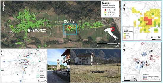
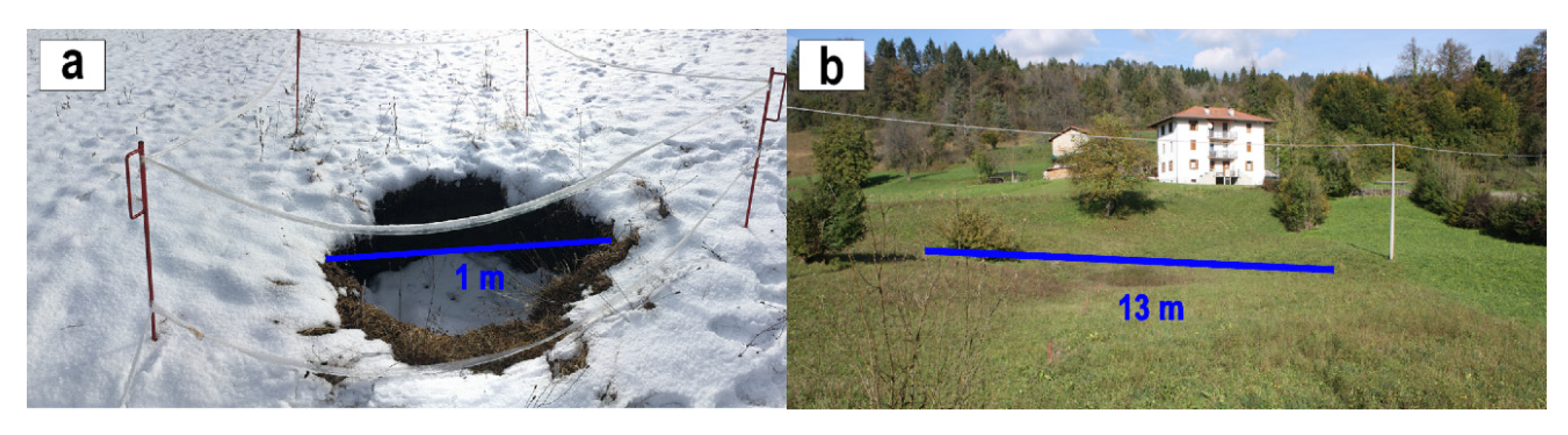
2. Study Area
- Red shales member (RBA1) with a thickness between 80 and 100 m, characterized by red shales and siltstones typical of a fluvial environment close to the coast;
- Gypsum and grey dolostones member (RBA2) characterized by a thickness of 350 m; it is primarily composed by grey and white saccharoid gypsum with marl inclusions at the top (Figure 3), yellowish dolomitic marls, and to a lesser extent, blackish or greenish clays and dark limestone in thin layers;
- Marls and dolostones member (RBA3) with a thickness of 180 m; it is characterized by grey dolostones often vacuolar and cataclastic, marls and multicolor clays close the depositional sequence.
3. Materials and Methods
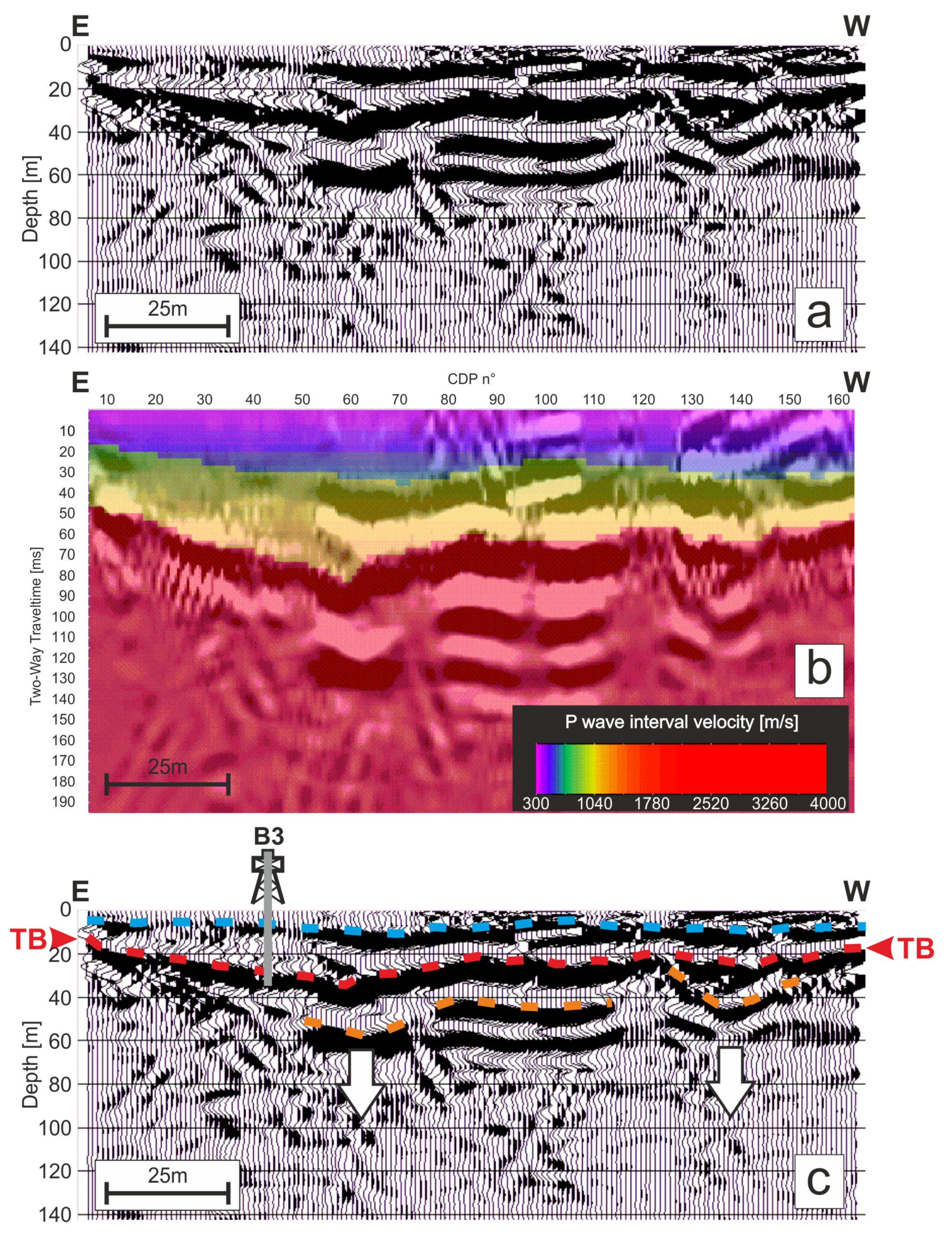
3.1. Reflection Seismics
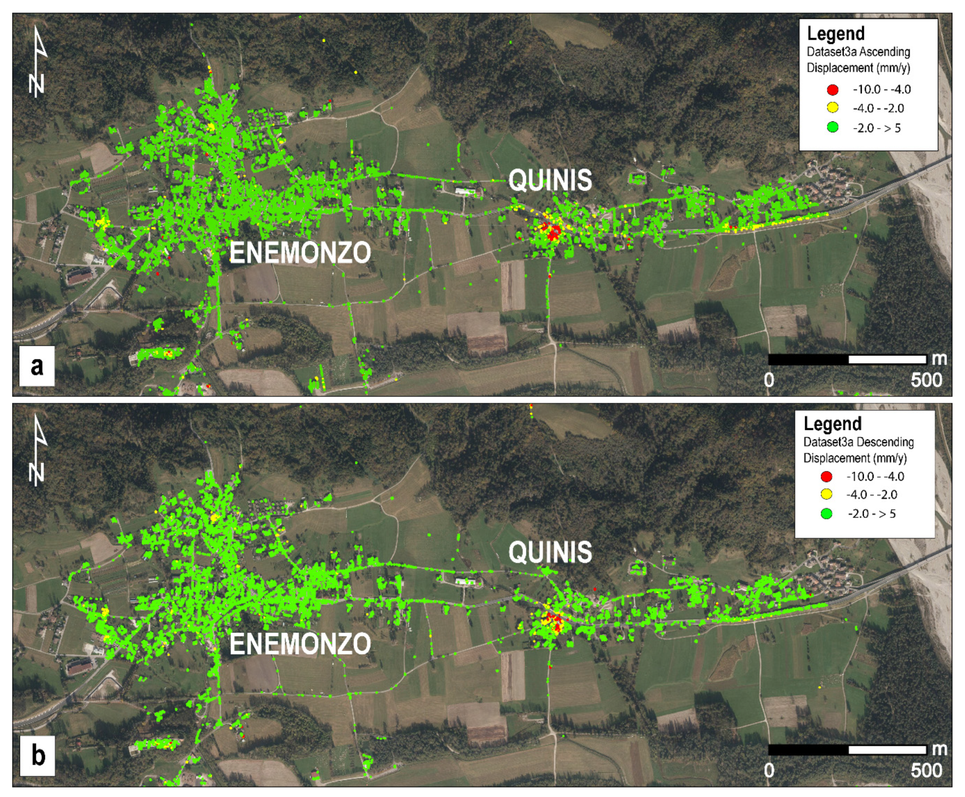
3.2. PS-InSAR
- An average velocity value (mm/y) referring to the displacement in LOS over the entire period of observation;
- An average velocity value (mm/y) referring to the displacement in LOS over each year;
- An estimated value of the cumulative displacement (mm);
- Standard deviation of the velocity with a mean value of 0.27 mm/y for the ascending dataset and 0.19 mm/y for the descending one.
3.3. Precise Geometric Leveling
3.4. 3D GPR
4. Results
4.1. Reflection Seismics
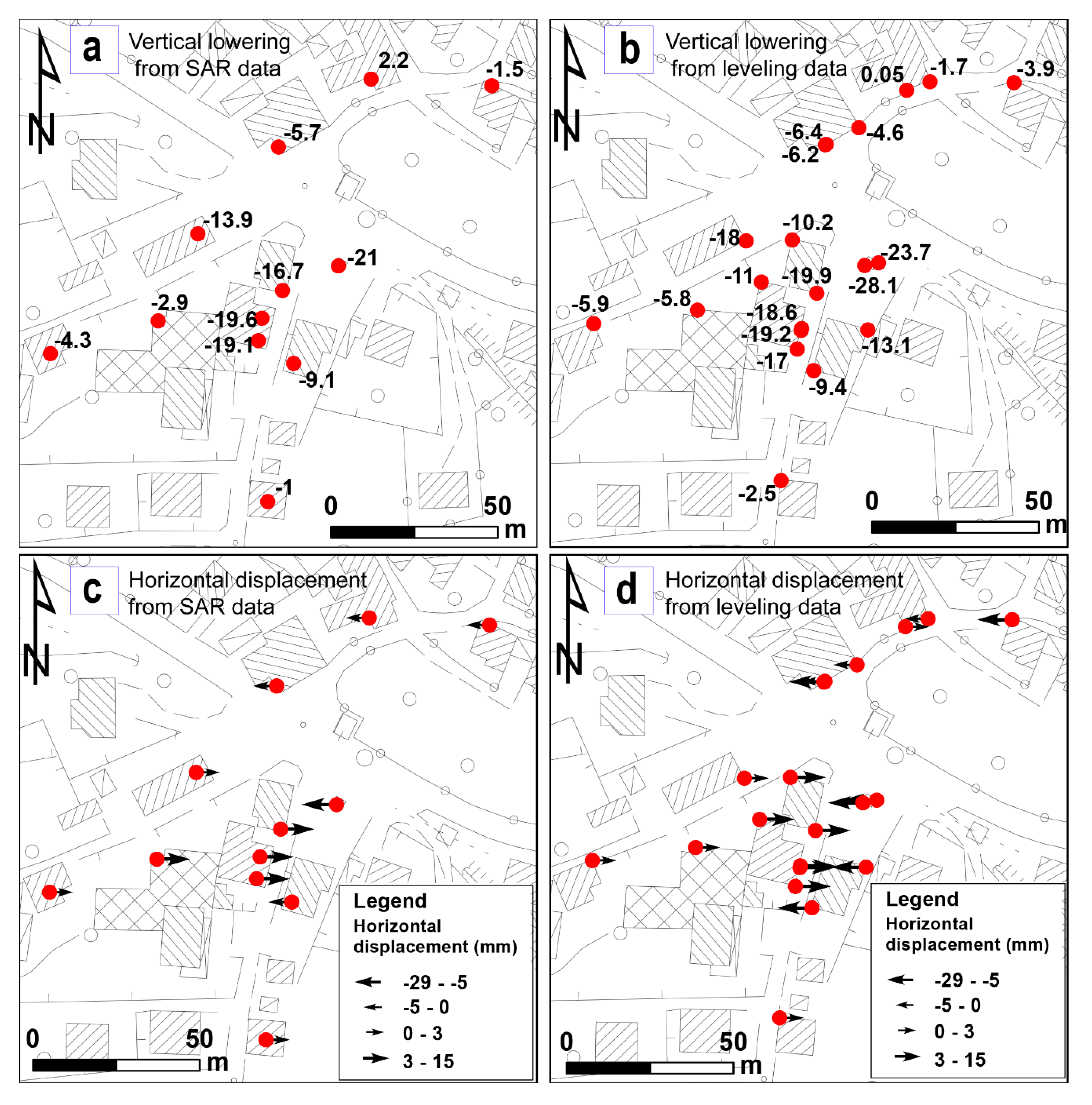
4.2. PS-InSAR and Leveling
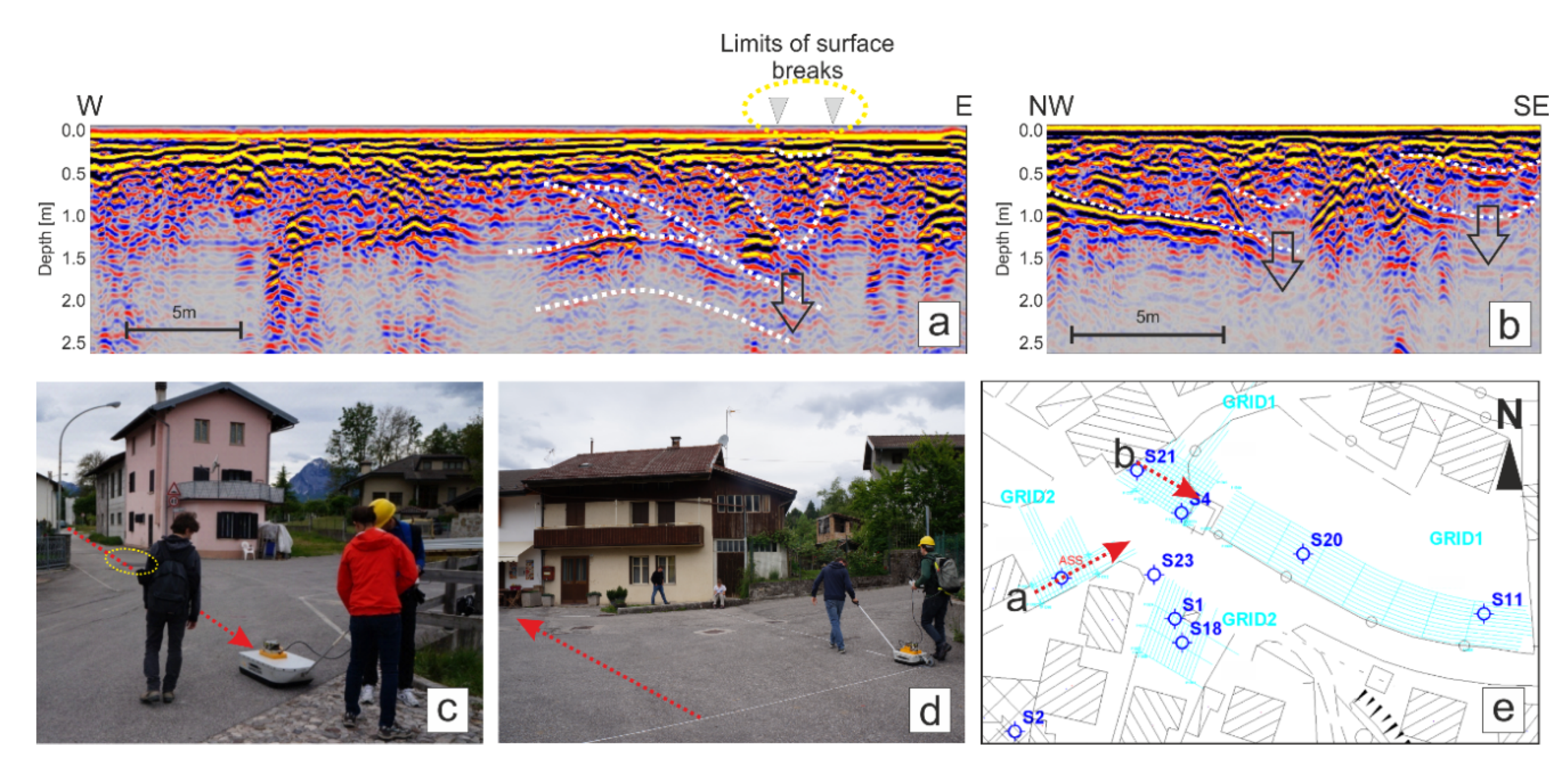
4.3. 3D GPR
5. Discussion
6. Conclusions
- (1)
- Image the most relevant subsurface features at a scale of tens of meters thanks to reflection seismics’ profiles (checked and validated by borehole stratigraphy);
- (2)
- Identify and map the zones with higher vertical movements thanks to the multi-year interferometric data analysis;
- (3)
- Cross-checking both vertical and horizontal movements by integrating repeated precise leveling measures with interferometry;
- (4)
- Highlight and map the main shallow depocenters thanks to full 3D GPR;
- (5)
- Obtain a summary map showing the highest vulnerable zone as a function of deformation thresholds set on the basis of the observations and peculiarities of the area (Figure 17).
Author Contributions
Funding
Acknowledgments
Conflicts of Interest
References
- Thierry, P.; Prunier-Leparmentier, A.M.; Lembezat, C.; Vanoudheusden, E.; Vernoux, J.F. 3D geological modelling at urban scale and mapping of ground movement susceptibility from gypsum dissolution: The Paris example (France). Eng. Geol. 2009, 105, 51–64. [Google Scholar] [CrossRef] [Green Version]
- Dahm, T.; Kühn, D.; Ohrnberger, M.; Kröger, J.; Wiederhold, H.; Reuther, C.-D.; Dehghani, A.; Scherbaum, F. Combining geophysical data sets to study the dynamics of shallow evaporites in urban environments: Application to Hamburg, Germany. Geophys. J. Int. 2010, 181, 154–172. [Google Scholar] [CrossRef] [Green Version]
- Paukstys, B.; Cooper, A.H.; Arustiene, J. Planning for gypsum geohazards in Lithuania and England. Eng. Geol. 1999, 52, 93–103. [Google Scholar] [CrossRef] [Green Version]
- Koutepov, V.M.; Mironov, O.K.; Tolmachev, V.V. Assessment of suffosion-related hazards in karst areas using GIS technology. Environ. Geol. 2008, 54, 957–962. [Google Scholar] [CrossRef]
- Gutiérrez, F.; Calaforra, J.M.; Cardona, F.; Ortí, F.; Durán, J.J.; Garay, P. Geological and environmental implications of the evaporite karst in Spain. Environ. Geol. 2008, 53, 951–965. [Google Scholar] [CrossRef]
- Sevil, J.; Gutiérrez, F.; Carmicer, C.; Carbonel, D.; Desir, G.; Garcià-Arnay, Á.; Guerrero, J. Characterizing and monitoring a high-risk sinkhole in an urban area underlain by salt through non-invasive methods: Detailed mapping, high-precision leveling and GPR. Eng. Geol. 2020, 272, 105641. [Google Scholar] [CrossRef]
- Cooper, A.H. Subsidence hazards caused by the dissolution of Permian gypsum in England: Geology, investigation and remediation. In Geohazards in Engineering Geology; Maund, J.G., Eddleston, M., Eds.; Geological Society of London: London, UK, 1998; pp. 265–275. [Google Scholar]
- Cooper, A.H.; Farrant, A.R.; Price, S.J. The use of karst geomorphology for planning, hazard avoidance and development in Great Britain. Geomorphology 2011, 134, 118–131. [Google Scholar] [CrossRef] [Green Version]
- Parise, M.; Qiriazi, P.; Sala, S. Natural and anthropogenic hazards in karst areas of Albania. Nat. Hazards Earth Syst. Sci. 2004, 4, 569–581. [Google Scholar] [CrossRef]
- Kuniansky, E.L.; Weary, D.L.; Kaufmann, J.E. The current status of mapping karst areas and availability of public sinkhole-risk resources in karst terrains of the United States. Hydrogeol. J. 2016, 24, 613–624. [Google Scholar] [CrossRef] [Green Version]
- Buttrick, D.B.; van Schalkwyk, A. Hazard and risk assessment for sinkhole formation on dolomite land in South Africa. Environ. Geol. 1998, 36, 170–178. [Google Scholar] [CrossRef]
- Nisio, S. I sinkholes nelle altre regioni. Mem. Descr. Carta Geol. It. 2008, 85, 419–426. (In Italian) [Google Scholar]
- De Waele, J.; Piccini, L.; Columbu, A.; Madonia, G.; Vattano, M.; Calligaris, C.; D’Angeli, I.M.; Parise, M.; Chiesi, M.; Sivelli, M.; et al. Evaporite karst in Italy: A review. Int. J. Speleol. 2017, 46, 137–168. [Google Scholar] [CrossRef] [Green Version]
- Calligaris, C.; Devoto, S.; Zini, L.; Cucchi, F. An integrated approach for investigations of ground subsidence phenomena in the Ovaro village (NE Italy). In Advance in Karst Science, Proceedings of EuroKarst 2016, Neuchâtel, Switzerland 2017; Renard, P., Bertrand, C., Eds.; Springer International Publishing: Geneva, Switzerland, 2017; Volume 8, pp. 71–77. [Google Scholar] [CrossRef]
- Calligaris, C.; Zini, L.; Nisio, S.; Piano, C. Sinkholes in the Friuli Venezia Giulia Region focus on the evaporites. J. Appl. Geology 2020, 5. [Google Scholar] [CrossRef]
- Cooper, A.H.; Gutiérrez, F. Dealing with gypsum karst problems: Hazards, environmental issues and planning. Treat. Geomorphol. 2013, 6, 451–462. [Google Scholar] [CrossRef] [Green Version]
- Frumkin, A. Salt karst. Treat. Geomorphol. 2013, 6, 407–424. [Google Scholar] [CrossRef]
- Zini, L.; Calligaris, C.; Forte, E.; Petronio, L.; Zavagno, E.; Boccali, C.; Cucchi, F. A multidisciplinary approach in sinkhole analysis: The Quinis village case study (NE-Italy). Eng. Geol. 2015, 197, 132–144. [Google Scholar] [CrossRef]
- Zhu, X.; Chen, W. Tiankengs in the karst of China. Cave Karst. Sci. 2005, 32, 55–66. [Google Scholar]
- Gutiérrez, F. Sinkhole Hazards. Oxford Res. Encycl. Nat. Hazard Sci. 2016. [Google Scholar] [CrossRef]
- Soldati, M.; Tonelli, C.; Galve, J.P. Geomorphological evolution of palaeosinkhole features in the Maltese Archipelago (Mediterranean Sea). Geogr. Fis. Dinam. Quat. 2013, 36, 189–198. [Google Scholar] [CrossRef]
- Nisio, S.; Caramanna, G.; Ciotoli, G. Sinkholes in Italy: First results on the inventory and analysis. In Natural and Anthropogenic Hazards in Karst Areas: Recognition, Analysis and Mitigation; Parise, M., Gunn, J., Eds.; Geological Society: London, UK, 2007; Volume 279, pp. 23–45. [Google Scholar] [CrossRef] [Green Version]
- Caramanna, G.; Ciotoli, G.; Nisio, S. A review of natural sinkhole phenomena in Italian plain areas. Nat. Hazards 2008, 45, 145–172. [Google Scholar] [CrossRef]
- Di Maggio, C.; Di Trapani, F.P.; Madonia, G.; Salvo, D.; Vattano, M. Primo contributo sui sinkhole nelle evaporiti della Sicilia (Italia)/First report on the sinkhole phenomena in the Sicilian evaporites (Italy). In Proceedings of the I sinkholes. Gli sprofondamenti catastrofici nell’ambiente naturale ed in quello antropizzato, Proceedings of the 2 Workshop Internazionale, Rome, Italy, 3–4 December 2009; ISPRA, Ed.; ISPRA: Roma, Italy, 2010; pp. 299–313. [Google Scholar]
- Iovine, G.; Parise, M.; Trocino, A. Instability phenomena in the evaporite karst of Calabria, Southern Italy. Zeit. Geomorphol. 2010, 54, 153–178. [Google Scholar] [CrossRef]
- Caporale, F.; De Venuto, G.; Leandro, G.; Spilotro, G. Interventi di mitigazione del rischio da sinkholes nell’area di Lesina marina (Provincia di Foggia, Italia). In Memorie Descrittive della Carta Geologica d’Italia; ISPRA, Ed.; ISPRA: Roma, Italy, 2013; Volume 93, pp. 121–142. (In Italian) [Google Scholar]
- Parise, M.; Vennari, C. A chronological catalogue of sinkholes in Italy: The first step toward a real evaluation of the sinkhole hazard. In Proceedings of the 13th Multidisciplinary Conference on Sinkholes and the Engineering and Environmental Impacts of Karst, Carlsbad, NM, USA, 6–10 May 2013; Land, L., Doctor, D.H., Stephenson, B., Eds.; NCKRI: Carlsbad, NM, USA, 2013; pp. 383–392. [Google Scholar] [CrossRef] [Green Version]
- Gortani, M. Le doline alluvionali. Nat. Mont. 1965, 3, 120–128. (In Italian) [Google Scholar]
- Marinelli, O. Fenomeni di tipo carsico nei terrazzi alluvionali della Valle del Tagliamento. Mem. Soc. Geogr. It. 1898, 8, 415–419. (In Italian) [Google Scholar]
- Fabbri, P.; Ortombina, M.; Piccinini, L.; Zampieri, D.; Zini, L. Hydrogeological spring characterization in the Vajont area. Ital. J. Eng. Geol. Environ. 2013, 6, 541–553. [Google Scholar] [CrossRef]
- Zini, L.; Calligaris, C.; Zavagno, E. Classical Karst hydrodynamics: A sheared aquifer within Italy and Slovenia. In Evolving Water Resources Systems: Understanding, Predicting and Managing Water-Society Interactions; Castellarin, A., Ceola, S., Toth, E., Montanari, A., Eds.; IAHS Publication: Bologna, Italy, June 2014; Volume 364, pp. 499–504. [Google Scholar] [CrossRef] [Green Version]
- Zini, L.; Casagrande, G.; Calligaris, C.; Cucchi, F.; Manca, P.; Treu, F.; Zavagno, E.; Biolchi, S. The Karst hydrostructure of the Mount Canin (Julian Alps, Italy and Slovenia). In Hydrogeological and Environmental Investigations in Karst Systems. Environmental Earth Sciences; Andreo, B., Carrasco, F., Durán, J.J., Jiménez, P., LaMoreaux, J., Eds.; Springer: Berlin/Heidelberg, Germany, 2015; Volume 1, pp. 219–226. [Google Scholar] [CrossRef]
- Zini, L.; Visintin, L.; Cucchi, F.; Boschin, W. Potential impact of a proposed railway tunnel on the karst environment: The example of Rosandra valley, Classical Karst Region, Italy-Slovenia. Acta Carsol. 2011, 40, 207–218. [Google Scholar] [CrossRef]
- Calligaris, C.; Boschin, W.; Cucchi, F.; Zini, L. The karst hydrostructure of the Verzegnis group (NE Italy). Carb. Evap. 2016, 31, 407–420. [Google Scholar] [CrossRef]
- Cucchi, F.; Finocchiaro, F.; Zini, L. Karst Geosites in NE Italy. Environ. Earth Sci. 2010, 393–398. [Google Scholar]
- Gutiérrez, F.; Parise, M.; De Waele, J.; Jourde, H. A review on natural and human-induced geohazards and impacts in karst. Earth Sci. Rev. 2014, 138, 61–88. [Google Scholar] [CrossRef]
- Theron, A.; Engelbrecht, J. The Role of Earth Observation, with a Focus on Sar Interferometry, for Sinkhole Hazard Assessment. Remote Sens. 2018, 10, 1506. [Google Scholar] [CrossRef] [Green Version]
- Jol, H.M. Ground Penetrating Radar Theory and Application, 1st ed.; Elsevier Science: Amsterdam, The Netherlands, 2009; p. 524. [Google Scholar] [CrossRef]
- Vaughan, D.G.; Corr, H.F.J.; Doake, C.S.M.; Waddington, E.D. Distortion of isochronous layers in ice revealed by ground-penetrating radar. Nature 1999, 398, 323–326. [Google Scholar] [CrossRef]
- Saarenketo, Y.; Scullion, T. Road evaluation with ground penetrating radar. J. Appl. Geophy 2000, 43, 119–138. [Google Scholar] [CrossRef]
- Zhao, E.; Tian, G.; Forte, E.; Pipan, M.; Wang, Y.; Li, X.; Shi, Z.; Liu, H. Advances in GPR data acquisition and analysis for archaeology. Geophys. J. Int. 2015, 202, 62–71. [Google Scholar] [CrossRef] [Green Version]
- Kruse, S.; Grasmueck, M.; Weiss, M.; Viggiano, D. Sinkhole structure imaging in covered Karst terrain. Geophys. Res. Lett. 2006, 33, L16405. [Google Scholar] [CrossRef] [Green Version]
- Ronen, A.; Ezersky, M.; Beck, A.; Gatenio, B.; Simhayov, B.R. Use of GPR method for prediction of sinkholes formation along the Dead Sea Shores, Israel. Geomorphology 2019, 328, 28–43. [Google Scholar] [CrossRef]
- Conway, B.; Cook, J. Monitoring evaporite karst activity and land subsidence in the Holbrook Basin, Arizona using interferometric synthetic aperture radar (InSAR). In Proceedings of the 13th Multidisciplinary Conference on Sinkholes and the Engineering and Environmental Impacts of Karst, Carlsbad, NM, USA, 6–10 May 2013; Land, L., Doctor, D.H., Stephenson, B., Eds.; NCKRI: Carlsbad, NM, USA, 2013; pp. 187–194. [Google Scholar] [CrossRef] [Green Version]
- Kim, J.W.; Lu, Z.; Degrandpre, K. Ongoing deformation of sinkholes in Wink, Texas, observed by time-series sentinel-1A SAR interferometry (preliminary results). Remote Sens. 2016, 8, 313. [Google Scholar] [CrossRef] [Green Version]
- Jones, C.E.; Blom, R.G. Bayou Corne, Louisiana, sinkhole: Precursory deformation measured by radar interferometry. Geology 2014, 42, 111–114. [Google Scholar] [CrossRef]
- Castañeda, C.; Gutiérrez, F.; Manunta, M.; Galve, J.P. DInSAR measurements of ground deformation by sinkholes, mining subsidence, and landslides, Ebro River, Spain. Earth Surf. Process. Landf. 2009, 34, 1562–1574. [Google Scholar] [CrossRef] [Green Version]
- Gutiérrez, F.; Galve, J.P.; Lucha, P.; Castañeda, C.; Bonachea, J.; Guerrero, J. Integrating geomorphological mapping, trenching, InSAR and GPR for the identification and characterization of sinkholes: A review and application in the mantled evaporite karst of the Ebro Valley (NE Spain). Geomorphology 2011, 134, 144–156. [Google Scholar] [CrossRef] [Green Version]
- Galve, J.P.; Castañeda, C.; Gutiérrez, F. Railway deformation detected by DInSAR over active sinkholes in the Ebro Valley evaporite karst, Spain. Nat. Hazards Earth Syst. Sci. 2015, 15, 2439–2448. [Google Scholar] [CrossRef] [Green Version]
- Cuenca, M.C.; Hanssen, R.F. Subsidence and uplift at Wassenberg, Germany due to coal mining using persistent scatterer interferometry. In Proceedings of the 13th FIG Symposium on Deformation Measurements and Analysis, Lisbon, Portugal, 12–15 May 2008; Gomez Garcia, V.A., Ed.; LNEC: Lisbon, Portugal, 2008; pp. 1–9. [Google Scholar]
- Cuenca, M.C. Improving Radar Interferometry for Monitoring Fault-Related Surface Deformation: Applications for the Roer Valley Graben and Coal Mine Induced Displacements in the Southern Netherlands. Ph.D. Thesis, Delft University of Technology, Delft, The Netherlands, 2 November 2012. [Google Scholar] [CrossRef]
- Chang, L.; Hanssen, R.F. Detection of cavity migration and sinkhole risk using radar interferometric time series. Remote Sens. Environ. 2014, 147, 56–64. [Google Scholar] [CrossRef]
- Nof, R.N.; Baer, G.; Ziv, A.; Raz, E.; Atzori, S.; Salvi, S. Sinkhole precursors along the Dead Sea, Israel, revealed by SAR interferometry. Geology 2013, 41, 1019–1022. [Google Scholar] [CrossRef]
- Theron, A.; Engelbrecht, J.; Kemp, J.; Kleynhans, W.; Turnbull, T. Detection of Sinkhole Precursors through SAR Interferometry: Radar and Geological Considerations. IEEE Geosci. Remote Sens. Lett. 2017, 14, 871–875. [Google Scholar] [CrossRef] [Green Version]
- Ferretti, A.; Basilico, M.; Novali, F.; Prati, C. Possibile utilizzo di dati radar satellitari per individuazione e monitoraggio di fenomeni di sinkholes. In Proceedings of the First Seminary on the State of the Art on Sinkhole Study and the role of National and Local Administration on Land Management, Rome, Italy; Nisio, S., Panetta, S., Vita, L., Eds.; APAT: Rome, Italy, 2004; pp. 331–340. [Google Scholar]
- Intrieri, E.; Gigli, G.; Nocentini, M.; Lombardi, L.; Mugnai, F.; Fidolini, F.; Casagli, N. Sinkhole monitoring and early warning: An experimental and successful GB-InSAR application. Geomorphology 2015, 241, 304–314. [Google Scholar] [CrossRef] [Green Version]
- Malinowska, A.A.; Witkowski, W.T.; Hejmanowski, R.; Chang, L.; van Leijen, F.J.; Hanssen, R.F. Sinkhole occurrence monitoring over shallow abandoned coal mines with satellite-based persistent scatterer interferometry. Eng. Geol. 2019, 262, 105336. [Google Scholar] [CrossRef]
- Vajedian, S.; Motagh, M. Extracting sinkhole features from time-series of TerraSAR-X/TanDEM-X data. ISPRS J. Photogramm. Remote Sens. 2019, 150, 274–284. [Google Scholar] [CrossRef]
- Novellino, A.; Cigna, F.; Brahmi, M.; Sowter, A.; Bateson, L.; Marsh, S. Assessing the feasibility of a national InSAR ground deformation map of Great Britain with Sentinel-1. Geosciences 2017, 7, 19. [Google Scholar] [CrossRef] [Green Version]
- Cosano, P.A.B. Rilievo Geologico dei Dintorni di Enemonzo (Carnia). Master’s Thesis, University of Milan, Milan, Italy, 1948. (In Italian). [Google Scholar]
- Venturini, C.; Spalletta, C.; Vai, G.B.; Pondrelli, M.; Delzotto, S.; Fontana, C.; Longo Salvador, G.; Carulli, G.B. Note Illustrative Carta geologica d’Italia alla scala 1:50.000 Foglio 031 Ampezzo; ISPRA: Rome, Italy, 2009; pp. 7–222. (In Italian) [Google Scholar]
- Carulli, G.B. Carta geologica del Friuli Venezia Giulia alla scala 1:150.000 e Note Illustrative; SELCA: Florence, Italy, 2006. (In Italian) [Google Scholar]
- Calligaris, C.; Ghezzi, L.; Petrini, R.; Lenaz, D.; Zini, L. Evaporite Dissolution Rate through an on-site Experiment into Piezometric Tubes Applied to the Real Case-Study of Quinis (NE Italy). Geosciences 2019, 9, 298. [Google Scholar] [CrossRef] [Green Version]
- Alsadi, H.N. Seismic Hydrocarbon Exploration 2D and 3D Techniques; Springer: Berlin, Germany, 2017; p. 331. ISBN 978-3-319-40325-6. [Google Scholar]
- Yilmaz, Ö. Seismic Data Analysis. Processing, Inversion, and Interpretation of Seismic Data, Society of Exploration Geophysicists; SEG: Tulsa, OH, USA, 2001; Volume 10, p. 2065. [Google Scholar] [CrossRef]
- Steeples, D.; Knapp, R.W.; McElwee, C.D. Seismic reflection investigations of sinkholes beneath Interstate Highway 70 in Kansas. Geophysics 1986, 51, 295. [Google Scholar] [CrossRef] [Green Version]
- Isiaka, A.I.; Durrheim, R.J.; Manzi, M.S.D. High-Resolution Seismic Reflection Investigation of Subsidence and Sinkholes at an Abandoned Coal Mine Site in South Africa. Pure Appl. Geophys. 2019, 176, 1531–1548. [Google Scholar] [CrossRef]
- Krawczyk, C.M.; Polom, U.; Trabs, S.; Dahm, T. Sinkholes in the city of Hamburg—New urban shear-wave reflection seismic system enables high-resolution imaging of subrosion structures. J. Appl. Geophy. 2012, 78, 133–143. [Google Scholar] [CrossRef]
- Wadas, S.H.; Tanner, D.C.; Polom, U.; Krawczyk, C.M. Structural analysis of S-wave seismics around an urban sinkhole: Evidence of enhanced dissolution in a strike-slip fault zone. Nat. Hazards Earth Syst. Sci. 2017, 17, 2335–2350. [Google Scholar] [CrossRef] [Green Version]
- Goldstein, R.M.; Zebker, H.A.; Werner, C.L. Satellite radar interferometry: Two-dimensional phase unwrapping. Radio Sci. 1988, 23, 713–720. [Google Scholar] [CrossRef] [Green Version]
- Bürgmann, R.; Rosen, P.A.; Fielding, E.J. Synthetic aperture radar interferometry to measure Earth’s surface topography and its deformation. Ann. Rev. Earth Planet. Sci. 2000, 28, 169–209. [Google Scholar] [CrossRef]
- Bamler, R.; Hartl, P. Synthetic aperture radar interferometry. InvPr 1998, 14, R1–R54. [Google Scholar] [CrossRef]
- Ferretti, A.; Prati, C.; Rocca, F. Permanent scatterers in SAR interferometry. IEEE Trans. Geosci. Remote Sens. 2001, 39, 8–20. [Google Scholar] [CrossRef]
- Bovenga, F.; Refice, A.; Nutricato, R.; Guerriero, L.; Chiaradia, M.T. SPINUA: A flexible processing chain for ERS/ENVISAT long term interferometry. In Proceedings of the ESA-ENVISAT Symposium 2004, Salzburg, Austria, 6–10 September 2004; Lacoste, H., Ouwehand, L., Eds.; Published on CD-Rom, 2004; pp. 1–6, Bibcode: 2005ESASP.572E.76B. Available online: https://www.scopus.com/inward/record.uri?eid=2-s2.0-23844488451&partnerID=40&md5=66fccec6df471bf259e63560d778dd1b (accessed on 19 November 2020).
- Merryman Boncori, J.P. Measuring Coseismic Deformation with Spaceborne Synthetic Aperture Radar: A Review. Front. Earth Sci. 2019, 7, 16. [Google Scholar] [CrossRef] [Green Version]
- Fialko, Y.; Simons, M.; Agnew, D. The complete (3-D) surface displacement field in the epicentral area of the 1999 M_W7. 1 Hector Mine Earthquake, California, from space geodetic observations. Geophys. Res. Lett. 2001, 28, 3063–3066. [Google Scholar] [CrossRef] [Green Version]
- Mehrabi, H.; Voosoghi, B.; Motagh, M.; Hanssen, R.F. Three-dimensional displacement fields from InSAR through Tikhonov regularization and least-squares variance component estimation. J. Surv. Eng. 2019, 145, 04019011. [Google Scholar] [CrossRef] [Green Version]
- Picco, S. Monitoraggio topografico. Dipartimento di Matematica e Geoscienze, Università degli Studi di Trieste (Italy); Unpublished work. 2014; 1–95. (In Italian) [Google Scholar]
- Trinks, I.; Gustafsson, J.; Emilsson, J.; Gustafsson, C.; Johansson, B.; Nissen, J. Efficient, large-scale archaeological prospection using a true 3D GPR array system. Archeosciences 2009, 33, 367–370. [Google Scholar] [CrossRef] [Green Version]
- Novo, A.; Dabas, M.; Morelli, G. The STREAM X Multichannel GPR System: First Test at Vieil-Evreux (France) and Comparison with Other Geophysical Data. Archaeol. Prospect. 2012, 19, 179–189. [Google Scholar] [CrossRef]
- Zhao, W.; Forte, E.; Pipan, M. Texture attribute analysis of GPR data for archaeological prospection. Pure Appl. Geophys. 2016, 173, 2237–2251. [Google Scholar] [CrossRef]
- Trinks, I.; Johansson, B.; Gustafsson, J.; Emilsson, J.; Friborg, J.; Gustafsson, C.; Nissen, J.; Hinterleitner, A. Efficient, large-scale archaeological prospection using a true three-dimensional ground-penetrating radar array system. Archaeol. Prospect. 2010, 17, 175–186. [Google Scholar] [CrossRef]
- Viberg, A.; Gustafsson, C.; Andrén, A. Multi-Channel Ground-Penetrating Radar Array Surveys of the Iron Age and Medieval Ringfort Bårby on the Island of Öland, Sweden. Remote Sens. 2020, 12, 227. [Google Scholar] [CrossRef] [Green Version]
- Grasmueck, M.; Novo, A. 3D GPR imaging of shallow plastic pipes, tree roots, and small objects. In Proceedings of the 16th International Conference on Ground Penetrating Radar (GPR), Hong Kong, China, 13–16 June 2016; pp. 1–6. [Google Scholar] [CrossRef]
- Muller, W.B. Semi-automatic determination of layer depth, permittivity and moisture content for unbound granular pavements using multi-offset 3-D GPR. Int. J. Pavement Eng. 2018, 21, 1281–1296. [Google Scholar] [CrossRef]
- Grasmueck, M.; Weger, R.; Horstmeyer, H. Full-resolution 3D GPR imaging. Geophysics 2005, 70, K12–K19. [Google Scholar] [CrossRef]
- McClymont, A.F.; Green, A.G.; Streich, R.; Horstmeyer, H.; Tronicke, J.; Nobes, D.C.; Pettinga, J.; Campbell, J.; Langridge, R. Visualization of active faults using geometric attributes of 3D GPR data: An example from the Alpine Fault Zone, New Zealand. Geophysics 2008, 73, 1MA-Z29(B11). [Google Scholar] [CrossRef] [Green Version]
- Chopra, S.; Marfurt, K.J. Seismic Attributes for Prospect Identification and Reservoir Characterization, Geophysical developments, n. 11; Society of Exploration Geophysicists: Tulsa, OH, USA, 2007; p. 481. ISBN 978-1-56080-141-2. [Google Scholar] [CrossRef]
- Zhao, W.; Forte, E.; Colucci, R.R.; Pipan, M. High-resolution glacier imaging and characterization by means of GPR attribute analysis. Geophys. J. Int. 2016, 206, 1366–1374. [Google Scholar] [CrossRef] [Green Version]
- Zini, L. Studi, analisi e coordinamento indagini volti alla definizione del fenomeno di emissione gassosa in Comune di Enemonzo, località Quinis, e delle eventuali correlazioni con i presenti fenomeni di sinkhole finalizzate alla valutazione della pericolosità associata nonché delle soluzioni tecniche di mitigazione o compensazione del dissesto. Dipartimento di Matematica e Geoscienze, Università degli Studi di Trieste (Italy); Unpublished work. 2015. (In Italian) [Google Scholar]


| Channel Number | up to 48 |
|---|---|
| Channel distance [m] | 2 |
| Shot interval [m] | 2 |
| Minimum Offset [m] | 1 |
| Maximum Offset [m] | 94 |
| Vertical stacking | 4 |
| Trace length [s] | 1 |
| Sampling interval [ms] | 0.25 |
| Data Editing |
|---|
| Geometry assignment and sorting |
| Static corrections |
| Coherent noise (ground roll) attenuation |
| Amplitude analysis and recovery |
| CMP velocity analysis and NMO correction |
| Stacking/weighted stack |
| Depth conversion |
Publisher’s Note: MDPI stays neutral with regard to jurisdictional claims in published maps and institutional affiliations. |
© 2020 by the authors. Licensee MDPI, Basel, Switzerland. This article is an open access article distributed under the terms and conditions of the Creative Commons Attribution (CC BY) license (http://creativecommons.org/licenses/by/4.0/).
Share and Cite
Busetti, A.; Calligaris, C.; Forte, E.; Areggi, G.; Mocnik, A.; Zini, L. Non-Invasive Methodological Approach to Detect and Characterize High-Risk Sinkholes in Urban Cover Evaporite Karst: Integrated Reflection Seismics, PS-InSAR, Leveling, 3D-GPR and Ancillary Data. A NE Italian Case Study. Remote Sens. 2020, 12, 3814. https://doi.org/10.3390/rs12223814
Busetti A, Calligaris C, Forte E, Areggi G, Mocnik A, Zini L. Non-Invasive Methodological Approach to Detect and Characterize High-Risk Sinkholes in Urban Cover Evaporite Karst: Integrated Reflection Seismics, PS-InSAR, Leveling, 3D-GPR and Ancillary Data. A NE Italian Case Study. Remote Sensing. 2020; 12(22):3814. https://doi.org/10.3390/rs12223814
Chicago/Turabian StyleBusetti, Alice, Chiara Calligaris, Emanuele Forte, Giulia Areggi, Arianna Mocnik, and Luca Zini. 2020. "Non-Invasive Methodological Approach to Detect and Characterize High-Risk Sinkholes in Urban Cover Evaporite Karst: Integrated Reflection Seismics, PS-InSAR, Leveling, 3D-GPR and Ancillary Data. A NE Italian Case Study" Remote Sensing 12, no. 22: 3814. https://doi.org/10.3390/rs12223814