1. Introduction
Worldwide, forests disappear at alarming rates. In the last decade, the average annual net forest/non-forest conversion loss was estimated at 4.74 million ha [
1]. Degradation of remaining natural forests is another major concern. A recent study of the Amazon region showed that losses in carbon were almost evenly split between cases attributable to forest conversion (e.g., biomass removals associated with commodity-driven deforestation) and cases due to forest degradation and disturbance (e.g., biomass reductions attributable to selective logging, drought, wildfire, etc.) [
2]. Less well-known, but of equal concern, are losses of peat underneath tropical peat swamp forests. The largest tropical peat deposits are found in Indonesia, the Peruvian Amazon, and the Congo Basin, accounting for a total of approximately100 gigatons carbon (GtC), equal to 25% of the carbon stock stored globally in biomass [
3,
4,
5]. For example, in degraded peat swamp forests in Indonesia, on average, approximately 0.4 GtC is lost annually because of oxidization and fires [
6]. Forest loss, forest degradation, and peat degradation are important components of carbon accounting. The Intergovernmental Panel on Climate Change (IPCC) recently released the 2019 Refinement to the 2006 IPCC Guidelines for National Greenhouse Gas Inventories, where the use of Earth observation data plays a prominent role [
7]. In addition to its role in carbon accounting, timely information on forest change is needed in support of other applications, such as forest management and peatland restoration. Optical satellite data have been used for decades for forest-change monitoring. Cloud cover, which can be very persistent in tropical rainforests, may pose problems when continuous timelines and timeliness of information is important. Radar data, such as Sentinel-1 data, offers an alternative. Radar’s independence of cloud cover is a clear advantage. However, this may not be the only advantage, as is explored later in this paper.
Deforestation is commonly defined as land-use change from forest land to any other non-forest land-use category and forest degradation as long-term loss of forest carbon stocks, as well as forest values without land-use, change [
8,
9,
10,
11]. However, quantitative criteria to describe forest degradation are still under discussion. Specification of thresholds for carbon stock loss and minimum area and time affected are not given, but are mandatory to apply such a definition [
9,
10,
11]. Deforestation detection (with optical data) is based on the easy differentiation between forest and non-forest classes, such as open areas, bare soil, agriculture, and settlements. Commonly used methods are based on sub-pixel approaches like spectral mixture analysis, which are also used to assess proxies of forest degradation [
12,
13,
14,
15]. The abovementioned recent study of the Amazon was based on MODIS data at ∼500 m resolution [
2]. It states that applying higher-resolution satellite data (e.g., 30 m Landsat imagery) would reduce uncertainty in carbon loss estimates, in particular, from degradation and disturbance. Another study, based on Landsat, mentions that subtle degradation signals are not easy to detect and are quickly lost over time due to fast re-vegetation [
16]. This would mean that significant loss of carbon could remain undetected. Obviously, higher spatial resolution provides more detail; however, regrowth or remaining understory can limit disturbance detection. Radar imaging is fundamentally different in several ways and can also be used to detect subtle patterns of forest disturbance, such as patterns caused by selective logging. Good results have been obtained with airborne radar [
17], and high-resolution satellite radar data, such as COSMO-SkyMed spotlight data [
18] and TerraSAR-X 3 m stripmap data [
19,
20]. However, such data types are not practical for wide-area monitoring applications. Coarser resolution radar data, such as the Sentinel-1 IW data, may offer a good alternative.
Forest disturbance, either through forest loss or drainage, can result in tropical peat disturbance. Peat swamp forests are among the world’s most threatened and least known ecosystems. In Southeast Asia, large areas of peat swamp forest have been drained, deforested (for timber), converted for agricultural projects (even though the soil is too acid), or are converted into plantations (such as oil palm, acacia, and Borneo rubber), even though peat systems are fragile and sensitive to hydrological disturbance (e.g., see Reference [
21]). Drainage through canalization has frequently and severely disrupted groundwater-level dynamics. Besides resulting in CO
2 emissions due to oxidization [
22,
23], this process makes them particularly vulnerable to fire, especially during ‘El Niño’ years [
24]. Emissions from the fires in Indonesia during 1997–1998, for example, have been estimated to be 0.8–2.5 GtC [
25,
26]. Water management is essential in addressing these disturbances. Indonesia currently makes efforts to restore degraded peatlands by “re-wetting”, blocking canals and promoting paludiculture. For these vast areas, near-real-time (NRT) information is needed on the construction of new drainage canals in the forest, which are often illegal and a precursor to further forest and peat disturbance. This is currently achieved by using SPOT-6/7 and Pleiades data, even though costs and cloud cover pose severe limitations.
Wide-area and spatially detailed NRT data are needed not only for tropical peatland management and restoration. Other sectors needing such data include law enforcement, national forest monitoring systems, and indigenous communities; MRV systems, carbon accounting, and REDD+ projects; sustainable development of timber trade, forest plantations, and other commodities; protection of conservation areas, biodiversity, and ecological corridors; and early warning and disaster management [
1,
10,
27,
28,
29,
30].
Several wide-area NRT systems already exist. Since 2004, near-real-time deforestation monitoring over the Brazilian Amazon has been carried out by INPE based on the Real Time Deforestation Detection System (DETER) program. The system currently uses the optical AWiFS data with 56 m spatial resolution and five-day temporal resolution [
31]. Because cloud cover poses a problem, the JJ-FAST system is considered as an additional NRT data source [
32]. The JJ-FAST system is based on ALOS PALSAR-2 ScanSAR data and is the first SAR-based global early warning system for tropical forests (covering 77 countries) [
33,
34]. It currently offers deforestation data every 1.5 months, at a minimum mapping unit (MMU) of 2 ha. Validation based on Landsat data provided by the GLAD system [
15] shows an overall user accuracy of 66.7% [
35]. The ALOS PALSAR observation strategy was designed to provide consistent wall-to-wall observations, at fine resolution, of almost all land areas on Earth, on a repetitive basis [
36]. In addition to providing the data for the JJ-FAST system, it is used to make annual global forest/non-forest maps [
37] and provide insight in the spatiotemporal radar backscatter variation of tropical forests [
38]. The L-band variability is relatively low for (dryland) tropical rainforest, higher for tropical moist deciduous forest and highest for tropical dry forest (for HH-polarization up to 3.5 dB standard deviation). The variability is also high for wetlands, such as peat swamp and floodplain forests [
38]. Moreover, for C-band data, spatiotemporal backscatter variation of tropical rainforest is low [
39] and can be substantial for tropical dry forest [
40].
Though L-band radar, in general, provides better contrast between forest and non-forest classes [
41,
42,
43,
44,
45]; C-band radar also seems well suitable for forest-change monitoring. From an operational point-of-view, this is particularly true for the Sentinel-1 radar, which reliably provides free medium-resolution data with a global coverage at a 6- or 12-day repeat cycle. From a technical point-of-view, there are a few challenges. (1) The first is the contrast between forest and non-forest, which, compared to L-band, is often low and of short duration (because of regrowth). (2) The spatiotemporal variability of forest can be substantial, notably for wetland forests; however, it seems lower than for L-band. (3) Spatial co-registration, with optical data and other radar, is difficult because of forest height, and limitations of available DEMs and radar parallaxes. This is especially true for the finer details, such as forest edges and disturbances. (4) Radar imaging is fundamentally different from optical imaging. Together with the previous issue, this complicates validation based on other satellite data. (5) Moreover, as stated in Reference [
32], “radar image analysis must be conducted carefully because there is no single pattern of deforestation in the Brazilian Amazon”. This is also the case for other tropical rainforest areas. Results depend on forest and terrain type and other environmental conditions, as discussed in this paper.
Several recent studies discuss the appropriateness of Sentinel-1 for forest/non-forest discrimination and deforestation detection. For a dryland forest site in the Peruvian Amazon, deforestation could be detected successfully (detection rate 95%) based on time-series analysis of radar shadows and the combined use of ascending and descending observations [
43]. In Reference [
44], several methods for forest/non-forest classification for a wide range of forest types are discussed. Classification accuracies for the tropical rainforest sites in this study are up to 81.6% (Sumatra) and up to 88.6% (Colombia). In Reference [
45] the potential of time-series and recurrence metrics for deforestation mapping at test sites in Mexico is discussed. In Reference [
46], for a site in the Amazon, it is shown that (time-series of) interferometric coherence has potential for deforestation detection.
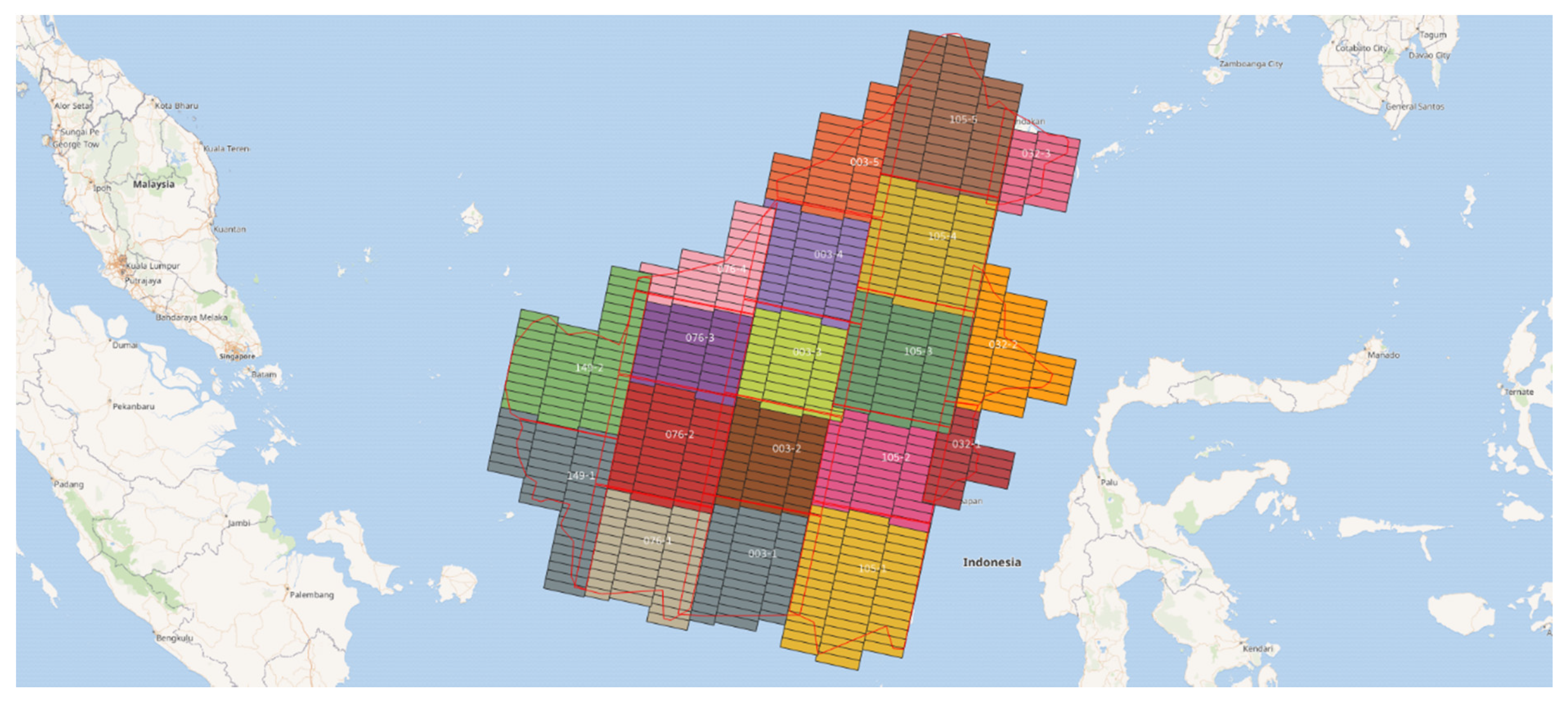
The objective of this paper is to discuss the suitability of Sentinel-1 radar for wide-area, NRT monitoring of tropical forest change in terms of deforestation and degradation, for a variety of landscapes in Indonesia and the Amazon, including tropical peat swamp forest landscapes. This requires clear definitions of forest, deforestation, degradation, and disturbance. However, users in different countries and disciplines use different definitions. It is therefore practical to have a flexible system that can be adapted to the needs of the user. It is also necessary to indicate the limitations of such a system. In this paper, certain default settings and definitions are used. The forest class includes undisturbed and disturbed natural forest and excludes forest plantations, such as acacia, rubber, and eucalypt. Deforestation is defined as clear-cut areas exceeding a certain size. The default threshold is arbitrarily set at 1.0 ha, except for peat swamp forest, where 0.3 ha is used. Any detected forest loss smaller than the default size is labelled as degradation. Degradation in degraded forests is mapped as the additional degradation since the start of the monitoring. The defaults values for the change detection algorithms used in this study were established during earlier work in Malaysia and Sumatra and seem generally applicable in all areas studied so far, including the Guianas, Gabon, and the areas validated in this paper. Special characteristics of tropical peat swamp forests, viz, the flat terrain and occurrence of long and narrow straight gaps caused by drainage canal construction, form ideal conditions for theoretical studies relevant for development of models to quantify degradation.
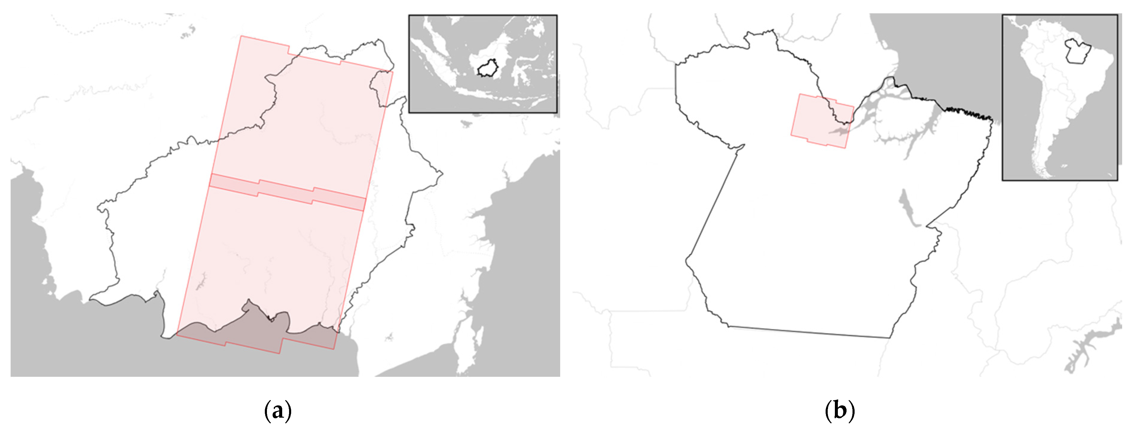
Section 2.1 introduces the study sites and supporting data.
Section 2.2,
Section 2.3 and
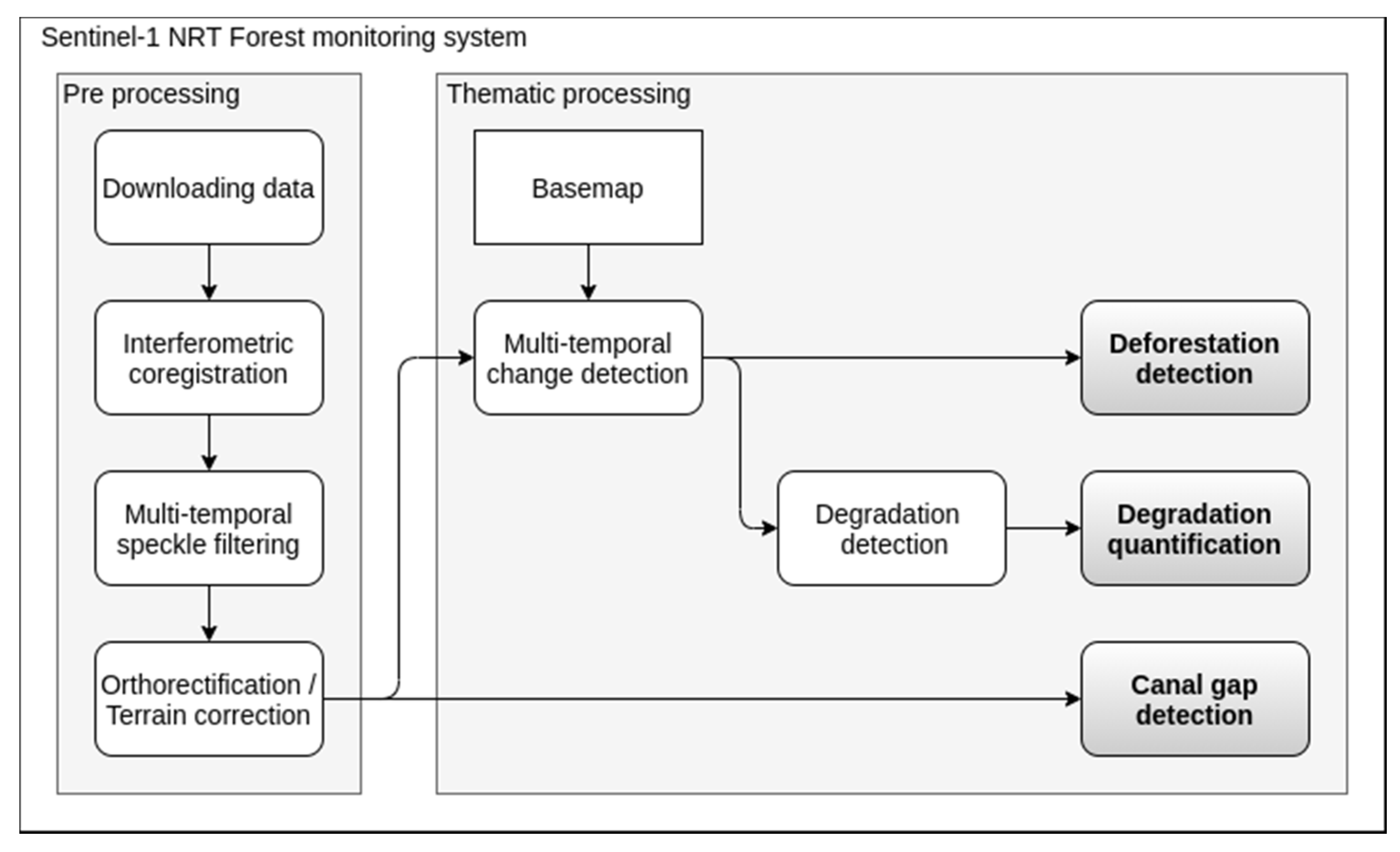
Section 2.4 describe physical background, system design considerations, and types of errors and summarize system components.
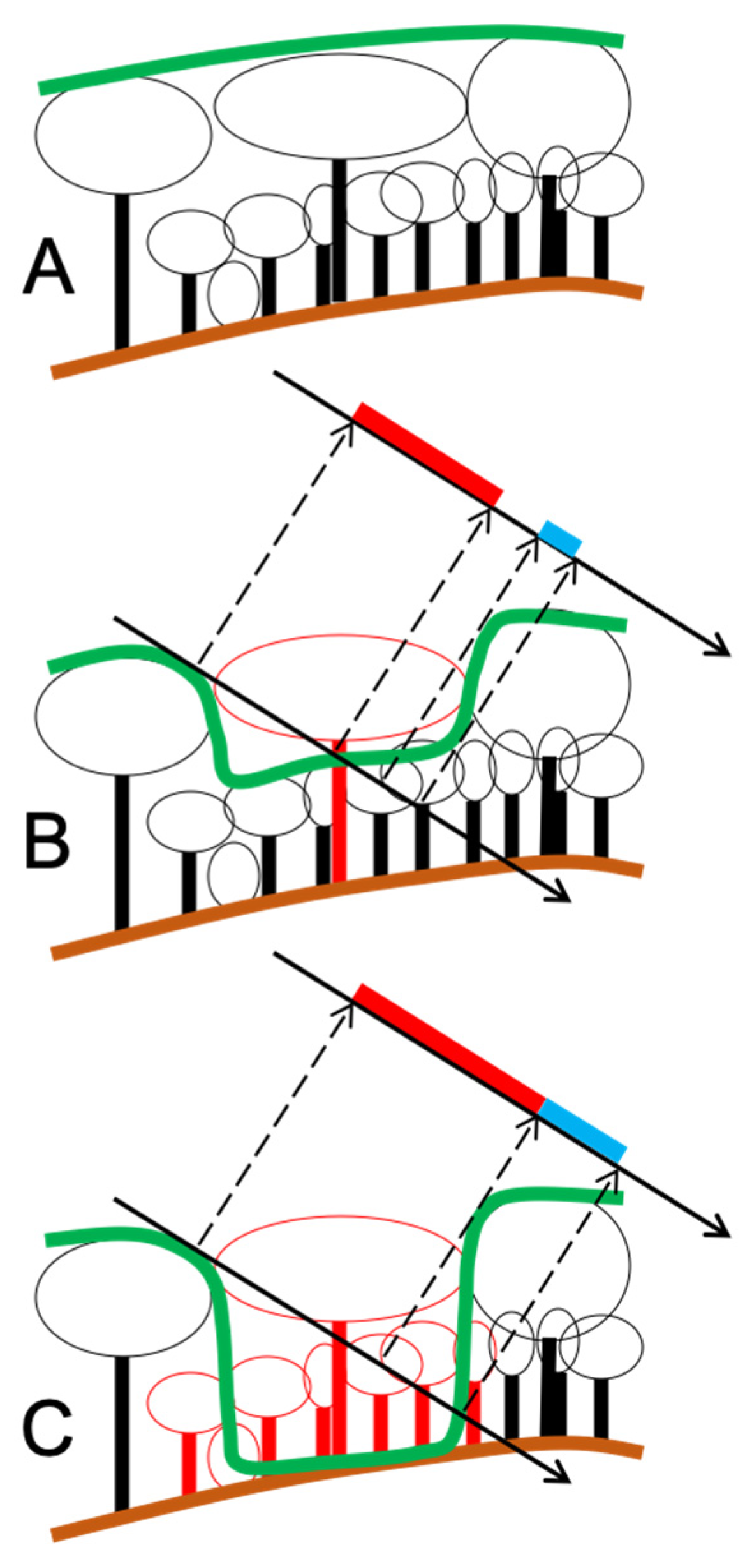
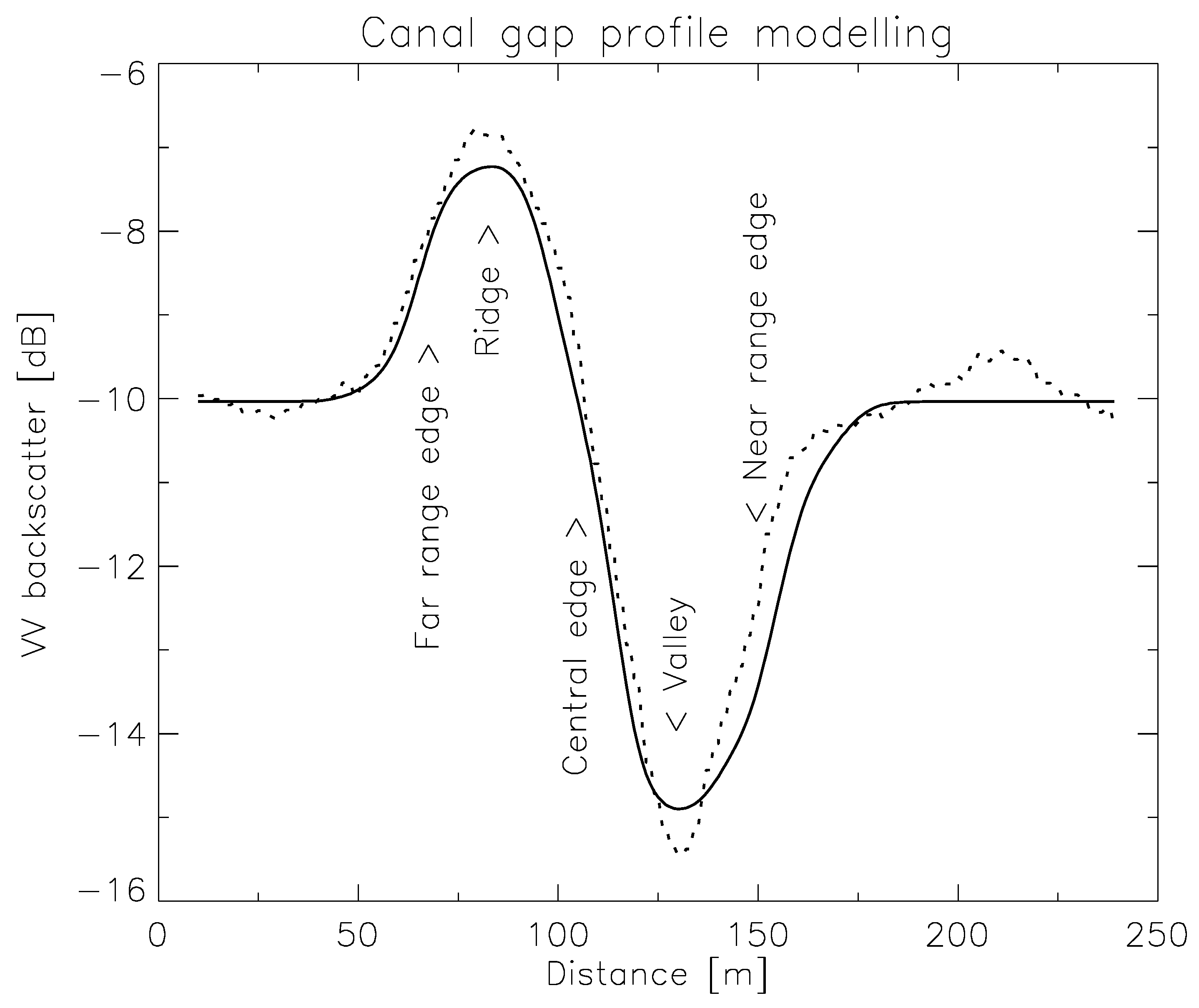
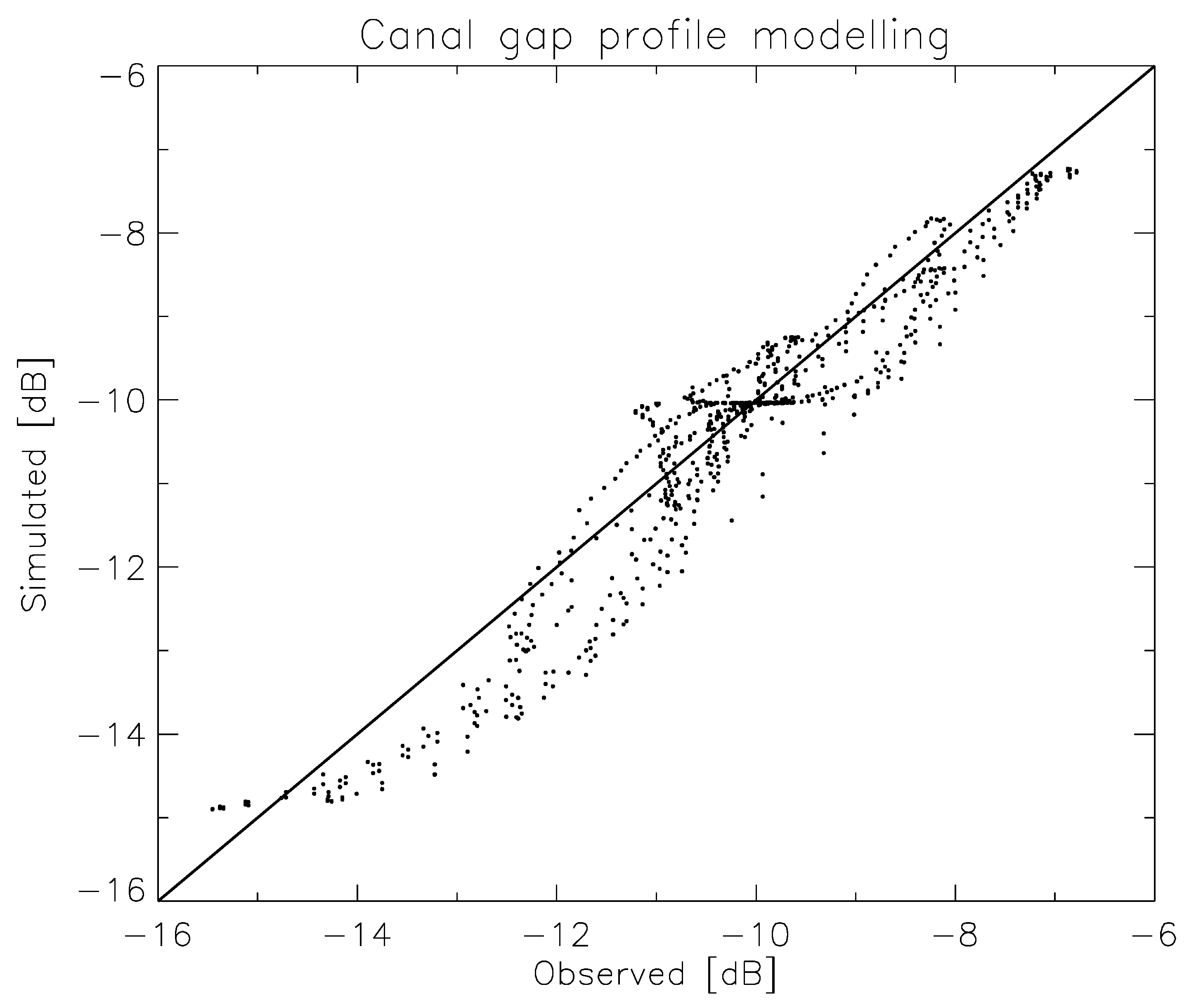
Section 2.5 provides a theoretical background for the radar imaging of linear canopy gaps (roads and canals) and small canopy gaps (tree logging gap disturbances) and introduces a physical model for radar imaging at high-resolution.
Section 3 provides results for NRT canal gap detection, NRT deforestation monitoring, and NRT degradation monitoring. It also reflects on validation challenges.
Section 4 and
Section 5 provide a synthesis and the main conclusions. The system is tested for a range of tropical forest landscapes and seems to function well, even in challenging environments, such as mountain slopes and wetlands. In this paper, the term “landscape” is used in the context of an ecosystem approach and stands for a vast area with a mosaic of forest types.
4. Discussion
4.1. System and Disturbance Model
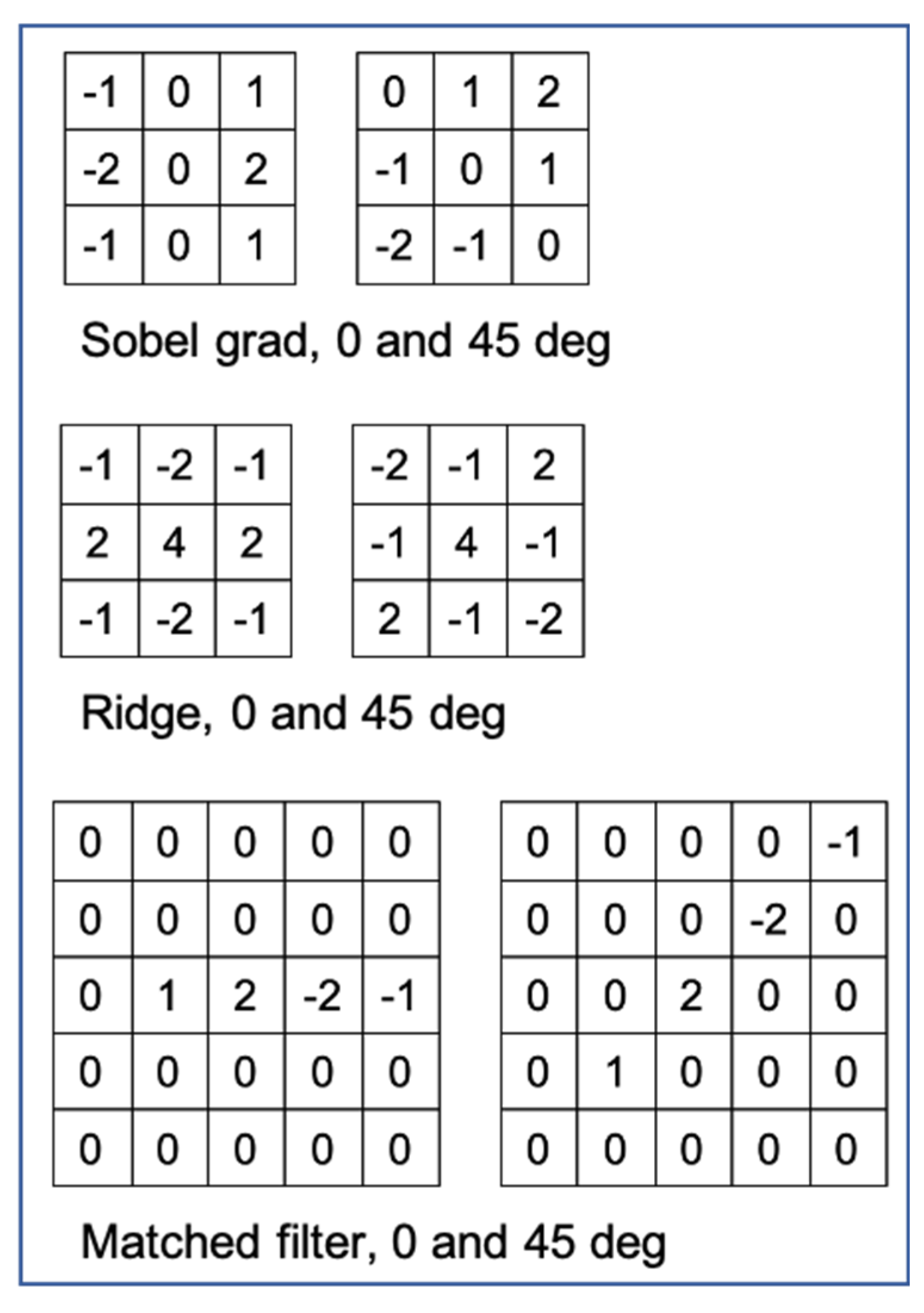
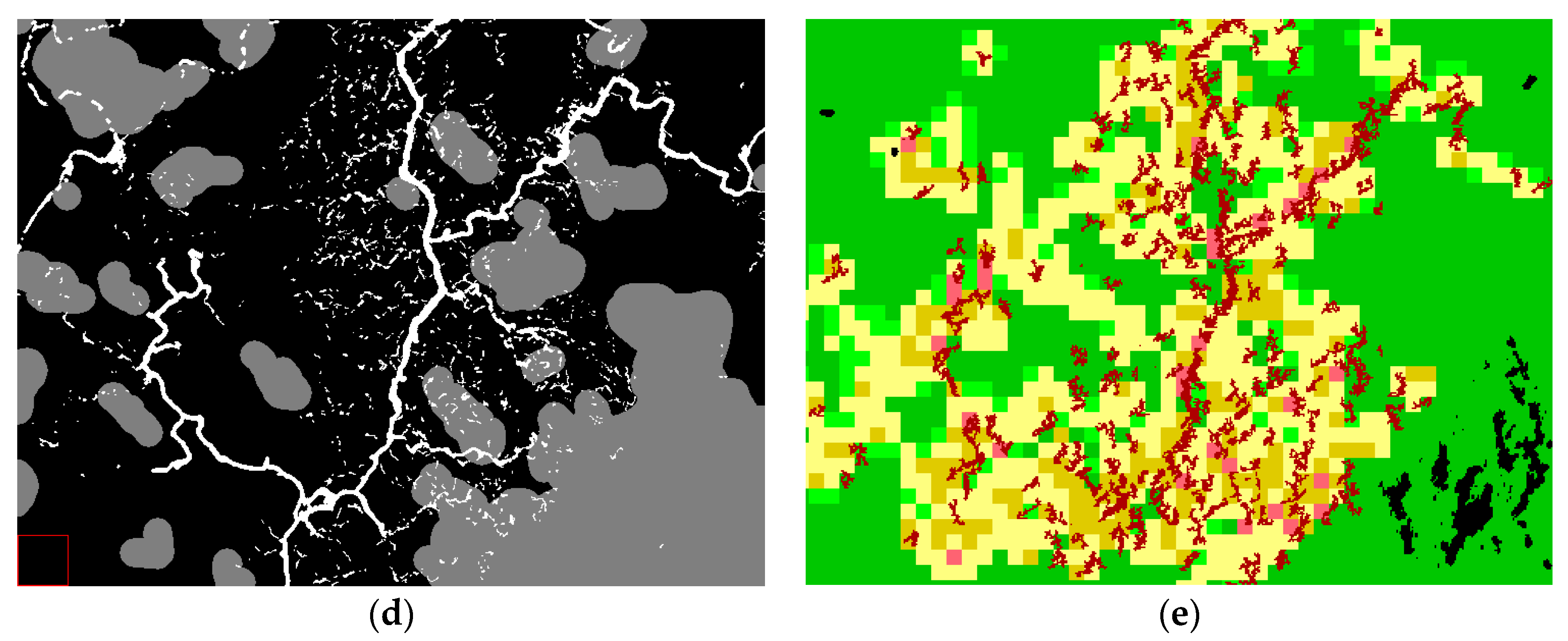
The Sentinel-1 NRT radar monitoring system is an automated system based on interferometric preprocessing and time-series analysis of small image segments, linear features, and small-scale disturbances. This results in a system that can accurately map different phenomena simultaneously, such as deforestation (clear-cut and fire scars), degradation, selective logging impact, and new narrow canals in peat swamp forest. Radar imaging of canal gaps and the canal-gap-detection mapping results were shown to be in agreement with a physical-interaction model. Small gaps caused by selective logging are too small to be detected individually; however, the same theoretical model (that describes canal gaps) can be used to quantify the canopy disturbance in a statistical sense. Therefore, change mapping is done in three fundamentally different ways. Deforestation is detected by using segment-based time-series analysis and uses a decrease of backscatter as an indicator of deforestation. Canal-gap detection is based on time-series analysis of linear features, using edge, line, and matched filters. Degradation is quantified by using a time-series analysis of textural change based on a physical model. These three approaches are not completely independent, not from a data processing point-of-view, nor from a forest-change-interpretation point-of-view.
Several examples of interdependency can be given. For deforestation mapping in peat swamp forests an MMU of 15 pixels (0.3 ha) applies. This means that wide canal gaps are often mapped as (a row of individual) segments. The same canal gaps show up in the canal gap maps as linear features. Of course, the dedicated canal gap product shows more canals, including some very narrow ones which are hardly visible in SPOT-6/7 data. Very small deforestation segments or very short canal gap detections are often part of degradation areas. At the Brazil test sites some areas of deforestation, the ones that gradually change from forest to low secondary forest without going through a bare soil stage, are not detected with the deforestation mapping approach. However, the near range edges of such areas are still visible as elongated segments, and parts of these areas are detected as degraded. Using such interdependencies explicitly may contribute to a better interpretation of ongoing forest-change processes.
4.2. Deforestation
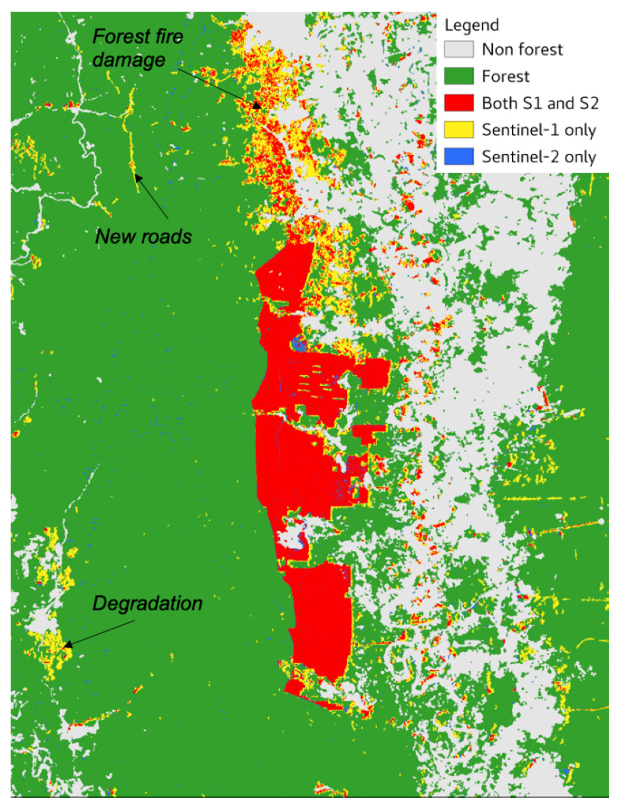
Deforestation detection success is evaluated by using results of a careful visual interpretation of Sentinel-2 time-series as a reference. These results are independent of any issues related to baseline class definitions and timing. In summary, for the Central Kalimantan landscapes, it is shown that the false alarm rate (FAR) is very low (less than 1%) and the missed detection rate (MDR) varies between 18.6% ± 1.0% and 1.9% ± 1.1% (90% confidence level). However, results also depend on user settings. FAR and MDR are interchangeable. Settings were selected to favor a low FAR at the expense of a slightly higher MDR. Another compromise to be made is between overall accuracy and timeliness. In other words, the faster the maps should be made available after radar observation, the lower the accuracy. Settings were selected to favor a relatively fast system, which results in significant detection delays in the map time-series. It was found that peatlands are a typical case where detection delays up to two months occur which are caused by the combination of rough soil surface and high soil moisture. This is causing the high MDR, but these missed detections are only temporary, not permanent. Other settings could decrease such delays to a few weeks. These delays were not found outside the peat areas or in the Amazon. Because of cloud cover, radar can be much faster than optical systems, but this cannot be validated by optical systems. It was found that radar very often detects deforestation two months and up to 10 months faster than optical systems.
4.3. Canal Gap Detection
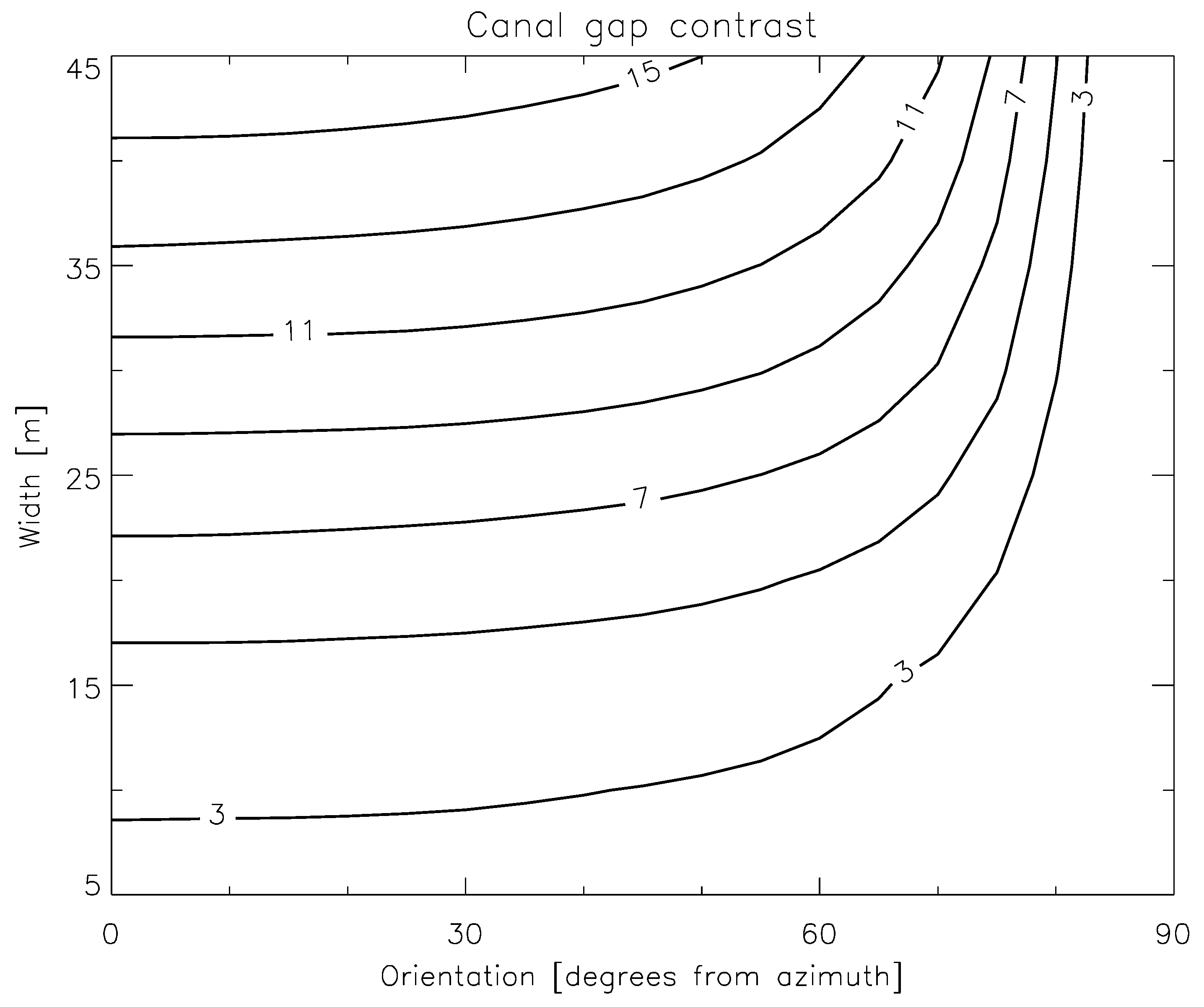
Results of visual interpretation of SPOT-6/7 images were used as reference. The overall detection rate is 85.5%; however, results strongly depend on canal gap orientation and, to a lesser extent, on canal gap width. Only for the smallest width class (5–10 m range) or for orientations of more than 80 degrees from azimuth direction, the accuracy drops below 50%. In total, 9.3 km of canal length was missed out of a total 64.2 km. Sentinel-1 canal gap detections which were not present in the initial reference set could be divided in two different categories. The first category consists of true canal gap segments very poorly visible in the SPOT images. These canal gaps are often narrow and often show regrowth. Once these canals are recognized in SPOT images, aided by the Sentinel-1 maps, additional visual interpretation is possible. In this study, 7.3 km of additional canal gaps could be found in the SPOT data. The second category consists of small canal gap segments in the NRT map which are not visible in the SPOT images, even after careful re-evaluation. A part of these false alarms is persistent while others disappear within two months. These persistent false-alarm detections, unlike the non-persistent false-alarm detections, are not located at random, but are located near canals and rivers or forest edges. These places are much more accessible and prone to illegal logging activities. Therefore, the false alarm rate of 9.5%, after approximately two months, could be divided into a non-persistent false alarm rate of 3.9% and a non-verifiable false alarm rate of 5.6%, which may relate to a large extent to true disturbances, such as illegal logging.
4.4. Degradation
Like for deforestation, degradation detection success is evaluated using results of a careful visual interpretation of Sentinel-2 time-series as a reference. Radar is a suitable instrument to quantify degradation. Unlike optical data, which detect degradation mainly by the signal fraction from the bare soil, the radar detects degradation by signals from gaps in the canopy, even when the understory still covers the soil. Therefore, the radar signal is very persistent (gaps in the upper canopy do not fill up fast), while the optical signal is visible for a short time window only (secondary regrowth on bare soil appears fast). The latter is even more troublesome when cloud cover is frequent. Validation is difficult using optical data since degradation is detected in a fundamentally different way and a lot of degradation is missed. Nevertheless, results are spatiotemporally consistent. It may be much better to use TerraSAR-X for validation of degradation, notably for quantitative validation. The result presented here, for Brazil, is based on limited data only but provides high spatiotemporal, as well as quantitative, agreement.
4.5. Comparison with Other Approaches Based on C-Band
Other existing methods based on C-band [
43,
44,
45,
46], which focus either on deforestation monitoring or forest/non-forest mapping, can be compared with the deforestation results presented here. The method for deforestation detection presented in Reference [
43] provides a similar accuracy level, however, requires both ascending and descending data. These are not available for most tropical forests, nor will they become available in the near future. The method for deforestation detection based on interferometric coherency [
46] is less accurate; however, it may provide useful additional information. The results of forest/non-forest classification presented in Reference [
44] also seem less accurate when used for the purpose of deforestation monitoring. The comparison with other systems is difficult because the system presented in this paper uses C-band for the monitoring part and a combination of L-band, C-band, and optical data for the (baseline) classification part.
5. Conclusions
Like JJ-FAST, the automated Sentinel-1 system presented here can be used for wide-area NRT forest-change monitoring. Results are available two days after satellite overpass, with higher spatial and temporal resolution and a high accuracy for deforestation detection. Unlike JJ-FAST, it utilizes multiple approaches for change detection, to allow monitoring of finer scaled features, such as narrow linear elements (roads and canals) and low-intensity degradation (selective logging). However, these refinements require the availability of a good forest baseline and system tuning to optimize it for local conditions, as well as local user requirements. The Sentinel-1 system is not meant primarily as a single system for pan-tropical coverage, but as a system to be operated and customized by local operators at the national level.
Though C-band, in general, has a lower forest/non-forest contrast than L-band, the Sentinel-1 radar in IW mode provides a higher temporal and spatial resolution than the PALSAR-2 ScanSAR mode, which makes Sentinel-1 equally suitable for the purpose of forest-change monitoring. One of the novelties in this paper is the use of the Sentinel-1 phase information for very precise co-registration (
Section 2.3), which allows for the detection of subtle changes.
Though tested for large areas in Indonesia and the Amazon, the validation requires more efforts, which should result in more refined local tuning. For example, a preliminary test for entire Borneo over the entire period revealed that there are still some deforested areas which were not detected but would have been detected with slightly different system settings. The quantitative estimation of degradation is difficult to validate with optical data. More work is needed, using extensive field data as reference, to calibrate the radar proxy for degradation and compare it with optical proxies.
Even though degradation information is still not yet properly calibrated and validated, several interesting applications emerge. For example, the result in
Figure 17 suggests that selective logging is not too intensive and is absent in the protected buffer zones along the river. This information is already helpful for planning field inspections in remote areas, certification, and transparency. Another example is early warning. Low-impact changes, such as new narrow roads, degradation, and small clear-cut areas in remote places are the first indications of potential future threats of forest-cover change. This information is already successfully used as input for predictive modelling based on machine learning by the World Wide Fund for Nature for the development of their Early Warning System (EWS) to predict deforestation [
29]. The data also support and could modernize conventional approaches based on hi-res optical data, to get more information out of these data, such as discussed above for the detection of narrow canal gaps in SPOT-6/7 data. Alternatively, hi-res optical data acquisition, for example, after a long period of cloud cover, could be focused on areas where change actually has occurred. The availability of free Sentinel-1 radar data with a systematic and complete coverage is a great asset for future development of efficient wide-area forest-monitoring systems.

 and
and 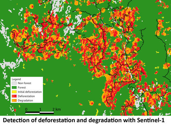


